ELISA_Visualizations

workflowr

• Summary
• Checks
• Past versions

Last updated: 2024-10-16

Checks: 7 0

Knit directory: test-3/

This reproducible R Markdown analysis was created with workflowr (version 1.7.1). The Checks tab describes the reproducibility checks that were applied when the results were created. The Past versions tab lists the development history.

---

R Markdown file: up-to-date

Great! Since the R Markdown file has been committed to the Git repository, you know the exact version of the code that produced these results.

Environment: empty

Great job! The global environment was empty. Objects defined in the global environment can affect the analysis in your R Markdown file in unknown ways. For reproduciblity it’s best to always run the code in an empty environment.

Seed: set.seed(20241016)

The command set.seed(20241016) was run prior to running the code in the R Markdown file. Setting a seed ensures that any results that rely on randomness, e.g. subsampling or permutations, are reproducible.

Session information: recorded

Great job! Recording the operating system, R version, and package versions is critical for reproducibility.

Cache: none

Nice! There were no cached chunks for this analysis, so you can be confident that you successfully produced the results during this run.

File paths: relative

Great job! Using relative paths to the files within your workflowr project makes it easier to run your code on other machines.

Repository version: 1953f30

Great! You are using Git for version control. Tracking code development and connecting the code version to the results is critical for reproducibility.

The results in this page were generated with repository version 1953f30. See the Past versions tab to see a history of the changes made to the R Markdown and HTML files.

Note that you need to be careful to ensure that all relevant files for the analysis have been committed to Git prior to generating the results (you can use wflow_publish or wflow_git_commit). workflowr only checks the R Markdown file, but you know if there are other scripts or data files that it depends on. Below is the status of the Git repository when the results were generated:

Ignored files:
    Ignored:    analysis/figure/

Unstaged changes:
    Modified:   analysis/ELISA_computation.Rmd

Note that any generated files, e.g. HTML, png, CSS, etc., are not included in this status report because it is ok for generated content to have uncommitted changes.

---

These are the previous versions of the repository in which changes were made to the R Markdown (analysis/ELISA_visualizations.Rmd) and HTML (docs/ELISA_visualizations.html) files. If you’ve configured a remote Git repository (see ?wflow_git_remote), click on the hyperlinks in the table below to view the files as they were in that past version.

File	Version	Author	Date	Message
Rmd	1953f30	Paloma	2024-10-16	wflow_publish("./analysis/ELISA_visualizations.Rmd")
html	b08a78b	Paloma	2024-10-16	Build site.
Rmd	0d06b46	Paloma	2024-10-16	wflow_publish("./analysis/ELISA_visualizations.Rmd")
Rmd	b03e143	Paloma	2024-10-16	creating plots
html	b03e143	Paloma	2024-10-16	creating plots
Rmd	2cbdcc9	Paloma	2024-10-16	merged data, cleaned, visualized some results
html	2cbdcc9	Paloma	2024-10-16	merged data, cleaned, visualized some results

---

Introduction

# load dataset
data <- read.csv("./data/Data_QC_filtered.csv")

#  since Buffer and spike are not continuous variables, change from numeric to factors
data$Buffer_nl <- as.factor(data$Buffer_nl)
data$Spike <- as.factor(data$Spike)

Calculating deviation from 50% binding

data$Binding_deviation <- abs(data$Binding.Perc - 50)
sorted_data <- data[order(data$Binding_deviation), ]

dim(sorted_data)

[1] 32 14

# View top results (closest to 50% Binding Percentage)
kable(sorted_data)

	Sample	Wells	Raw.OD	Binding.Perc	Concentration_pg.ml	Average_Conc_pg.ml	CV.Perc	SD	SEM	Weight_mg	Buffer_nl	Spike	Failed_samples	Binding_deviation
22	32	A11	0.656	50.0	1228.0	1197.0	3.690	44.20	31.30	37.1	250	0	NA	0.0
21	31	H9	0.701	51.2	1070.0	1149.0	9.750	112.00	79.20	21.2	60	0	NA	1.2
24	34	C11	0.687	51.7	1117.0	1124.0	0.867	9.74	6.89	35.5	250	0	NA	1.7
23	33	B11	0.696	52.3	1087.0	1100.0	1.730	19.10	13.50	33.8	250	0	NA	2.3
25	36	E11	0.695	53.2	1090.0	1062.0	3.680	39.10	27.60	31.2	250	0	NA	3.2
15	27	E9	0.610	46.0	1417.0	1393.0	2.430	33.80	23.90	21.6	60	0	NA	4.0
8	18	D7	0.734	56.0	967.1	955.4	1.740	16.60	11.70	30.8	250	0	NA	6.0
16	28	F9	0.757	59.5	901.0	839.7	10.300	86.70	61.30	23.2	250	0	NA	9.5
12	23	A8	0.809	60.9	766.3	793.6	4.880	38.70	27.40	24.6	250	0	NA	10.9
14	26	D9	0.477	37.3	2197.0	1991.0	14.600	291.00	206.00	20.2	60	0	NA	12.7
17	29	G9	0.518	36.2	1907.0	2072.0	11.200	232.00	164.00	36.5	60	0	NA	13.8
26	37	F11	0.482	36.1	2158.0	2076.0	5.620	117.00	82.50	30.8	60	0	NA	13.9
13	24	B9	0.835	64.8	705.5	680.2	5.260	35.80	25.30	20.4	250	0	NA	14.8
29	6	H3	0.490	34.7	2099.0	2204.0	6.750	149.00	105.00	13.7	60	1	NA	15.3
18	3	E3	0.478	33.9	2189.0	2287.0	6.090	139.00	98.50	11.0	60	1	NA	16.1
5	15	A7	0.888	66.2	592.9	643.6	11.100	71.60	50.70	12.0	60	0	NA	16.2
11	22	H7	0.453	33.0	2395.0	2377.0	1.030	24.50	17.40	21.5	250	1	NA	17.0
27	38	G11	0.429	32.5	2619.0	2444.0	10.200	248.00	176.00	34.7	60	0	NA	17.5
3	13	G5	0.451	32.1	2412.0	2477.0	3.680	91.10	64.40	16.8	250	1	NA	17.9
4	14	H5	0.437	31.8	2541.0	2504.0	2.110	52.90	37.40	13.8	250	1	NA	18.2
10	21	G7	0.425	31.6	2660.0	2540.0	6.630	169.00	119.00	28.0	250	1	NA	18.4
30	7	A5	0.436	30.5	2551.0	2669.0	6.250	167.00	118.00	16.4	60	1	NA	19.5
32	9	C5	0.432	30.3	2590.0	2693.0	5.460	147.00	104.00	19.2	250	1	NA	19.7
2	12	F5	0.422	30.0	2690.0	2728.0	1.920	52.50	37.10	24.1	250	1	NA	20.0
19	30A	A3	0.403	28.8	2899.0	2888.0	0.565	16.30	11.50	29.6	250	1	NA	21.2
1	11	E5	0.939	71.6	496.8	513.2	4.500	23.10	16.30	17.5	250	0	NA	21.6
28	5	G3	0.944	72.1	488.0	501.4	3.790	19.00	13.40	14.4	60	0	NA	22.1
6	16	B7	0.372	26.8	3297.0	3196.0	4.470	143.00	101.00	23.4	60	1	NA	23.2
9	19	E7	0.364	24.1	3413.0	3730.0	12.000	449.00	317.00	27.9	60	1	NA	25.9
31	8	B5	1.030	77.8	354.9	386.8	11.700	45.10	31.90	15.3	250	0	NA	27.8
20	30B	B3	1.050	81.1	314.1	324.9	4.700	15.30	10.80	29.6	250	0	ABOVE 80% binding	31.1
7	17	C7	1.080	84.3	278.0	270.6	3.860	10.50	7.39	24.5	60	0	ABOVE 80% binding	34.3

Scatterplots

Binding percentage

# Scatter plot of Binding Percentage vs Weight, 4 groups
ggplot(data, aes(x = Weight_mg, y = Binding.Perc, color = factor(Spike), shape = factor(Buffer_nl))) +
  geom_point(size = 3) +
  geom_smooth(method = "lm", se = FALSE, linewidth = 0.5) +  # Add a linear trend line
  labs(title = "Binding Percentage vs Weight, 4 groups",
       x = "Weight (mg)", y = "Binding Percentage") +
   scale_y_continuous(n.breaks = 10) +  
    geom_hline(yintercept = 50, linetype = "dashed", color = "gray", linewidth = 1) +  # Add horizontal line at y = 20
  theme_minimal()

`geom_smooth()` using formula = 'y ~ x'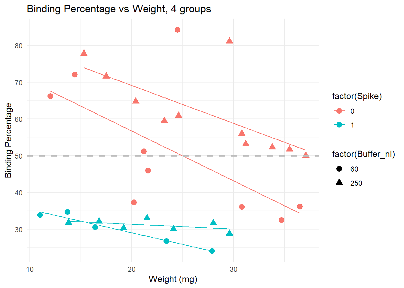

Past versions of unnamed-chunk-4-1.png

Version	Author	Date
b08a78b	Paloma	2024-10-16
b03e143	Paloma	2024-10-16

# Scatter plot of Binding Percentage vs Weight, 2 groups (Buffer)
ggplot(data, aes(x = Weight_mg, y = Binding.Perc, color = factor(Buffer_nl))) +
  geom_point(size = 3) +
  geom_smooth(method = "lm", se = FALSE, linewidth = 0.5) +  # Add a linear trend line
  labs(title = "Binding Percentage vs Weight, by Buffer",
       x = "Weight (mg)", y = "Binding Percentage") +
   scale_y_continuous(n.breaks = 10) +  
    geom_hline(yintercept = 50, linetype = "dashed", color = "gray", linewidth = 1) +  # Add horizontal line at y = 20
  theme_minimal()

`geom_smooth()` using formula = 'y ~ x'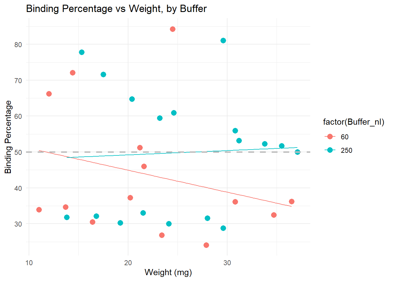

Past versions of unnamed-chunk-4-2.png

Version	Author	Date
b08a78b	Paloma	2024-10-16
b03e143	Paloma	2024-10-16

# Scatter plot of Binding Percentage vs Weight, 2 groups (Spike)
ggplot(data, aes(x = Weight_mg, y = Binding.Perc, shape = factor(Spike))) +
  geom_point(size = 3, colour = "cyan4") +
  geom_smooth(method = "lm", se = FALSE, linewidth = 0.5, colour = "cyan3") +  # Add a linear trend line
  labs(title = "Binding Percentage vs Weight, by Spike",
       x = "Weight (mg)", y = "Binding Percentage") +
   scale_y_continuous(n.breaks = 10) +  
    geom_hline(yintercept = 50, linetype = "dashed", color = "gray", linewidth = 1) +  # Add horizontal line at y = 20
  theme_minimal()

`geom_smooth()` using formula = 'y ~ x'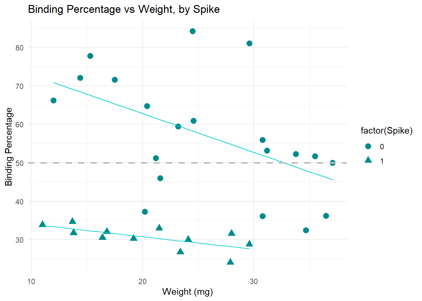

Past versions of unnamed-chunk-4-3.png

Version	Author	Date
b08a78b	Paloma	2024-10-16
b03e143	Paloma	2024-10-16

Coef. of variation percentage

# Scatterplot of CV Percentage vs Buffer & Spike
ggplot(data, aes(x = factor(Buffer_nl), y = CV.Perc, fill = factor(Spike))) +
  geom_boxplot() +
  labs(title = "Coef. of variation by Buffer and Spike",
       x = "Buffer (nl)", y = "Coef of variation %") +
   scale_y_continuous(n.breaks = 10) +  
  theme_minimal()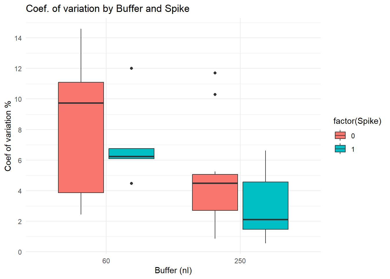

Past versions of unnamed-chunk-5-1.png

Version	Author	Date
b08a78b	Paloma	2024-10-16

# Scatter plot of Binding Percentage vs Weight, 4 groups
ggplot(data, aes(x = Weight_mg, y = CV.Perc, color = factor(Spike), shape = factor(Buffer_nl))) +
  geom_point(size = 3) +
  geom_smooth(method = "lm", se = FALSE, linewidth = 0.5) +  # Add a linear trend line
  labs(title = "Coef. of variation vs Weight, 4 groups",
       x = "Weight (mg)", y = "Coef of variation %") +
   scale_y_continuous(n.breaks = 10) +  
  theme_minimal()

`geom_smooth()` using formula = 'y ~ x'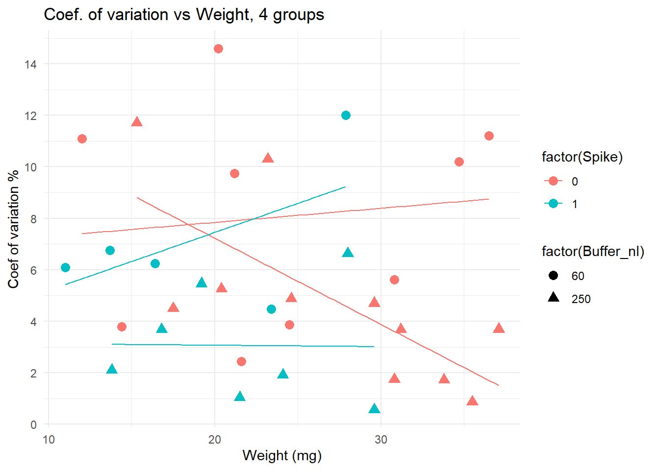

Past versions of unnamed-chunk-5-2.png

Version	Author	Date
b08a78b	Paloma	2024-10-16

Deviation from 50% binding

# Scatter plot of Binding Deviation vs Weight, 4 groups
ggplot(data, aes(x = Weight_mg, y = Binding_deviation, color = factor(Spike), shape = factor(Buffer_nl))) +
  geom_point(size = 3) +
  geom_smooth(method = "lm", se = FALSE, linewidth = 0.5) +  # Add a linear trend line
  labs(title = "Binding Deviation vs Weight, 4 groups",
       x = "Weight (mg)", y = "Binding Deviation") +
   scale_y_continuous(n.breaks = 10) +  
  theme_minimal()

`geom_smooth()` using formula = 'y ~ x'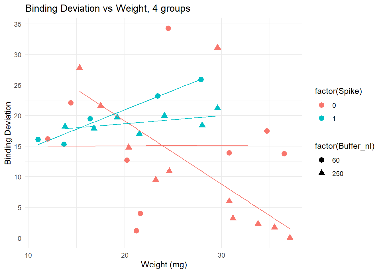

Past versions of unnamed-chunk-6-1.png

Version	Author	Date
b08a78b	Paloma	2024-10-16

# Scatter plot of Binding Deviation vs Weight, colored by Buffer
ggplot(data, aes(x = Weight_mg, y = Binding_deviation, color = factor(Buffer_nl))) +
  geom_point(size = 3) +
  geom_smooth(method = "lm", se = FALSE) +  # Add a linear trend line
  labs(title = "Binding Deviation vs Weight, colored by Buffer",
       x = "Weight (mg)", y = "Binding Percentage") +
   scale_y_continuous(n.breaks = 10) +  
  theme_minimal()

`geom_smooth()` using formula = 'y ~ x'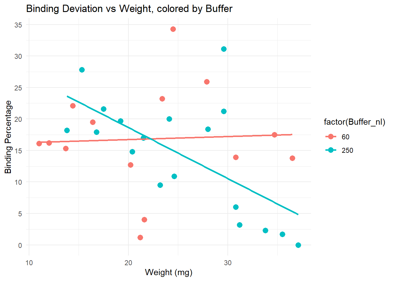

Past versions of unnamed-chunk-6-2.png

Version	Author	Date
b08a78b	Paloma	2024-10-16

# Scatter plot of Binding Deviation vs Weight, shape by Spike
ggplot(data, aes(x = Weight_mg, y = Binding_deviation, shape = factor(Spike))) +
  geom_point(size = 3, colour = "cyan4") + 
  geom_smooth(method = "lm", se = FALSE, linewidth = 0.5, colour = "cyan3") +  # Add a linear trend line
  labs(title = "Binding Deviation vs Weight, shape by Spike",
       x = "Weight (mg)", y = "Binding Deviation") +
   scale_y_continuous(n.breaks = 10) +  
  theme_minimal()

`geom_smooth()` using formula = 'y ~ x'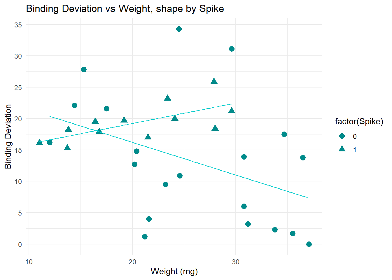

Past versions of unnamed-chunk-6-3.png

Version	Author	Date
b08a78b	Paloma	2024-10-16

Boxplots

Binding percentage

# Boxplot of Binding Percentage vs Buffer & Spike
ggplot(data, aes(x = factor(Buffer_nl), y = Binding.Perc, fill = factor(Spike))) +
  geom_boxplot() +
  labs(title = "Binding Percentage by Buffer and Spike",
       x = "Buffer (nl)", y = "Binding Percentage") +
   scale_y_continuous(n.breaks = 10) +  
      geom_hline(yintercept = 50, linetype = "dashed", color = "gray", linewidth = 1) + 
  theme_minimal()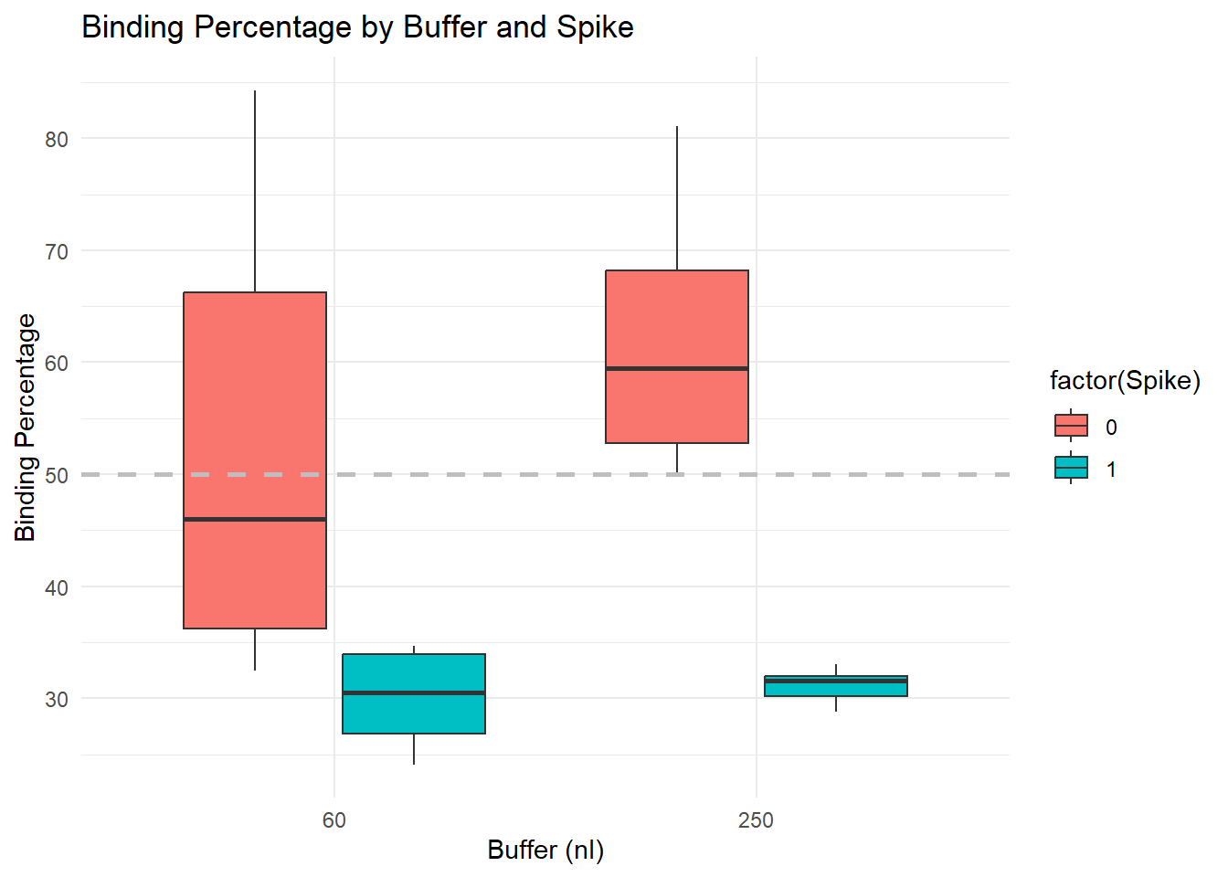

Past versions of unnamed-chunk-7-1.png

Version	Author	Date
b08a78b	Paloma	2024-10-16

# Boxplot of Binding Percentage vs Buffer
ggplot(data, aes(x = factor(Buffer_nl), y = Binding.Perc, fill = factor(Buffer_nl))) +
  geom_boxplot() +
  labs(title = "Binding Percentage by Buffer",
       x = "Buffer (nl)", y = "Bindings Percentage") +
   scale_y_continuous(n.breaks = 10) +  
      geom_hline(yintercept = 50, linetype = "dashed", color = "gray", linewidth = 1) + 
  theme_minimal()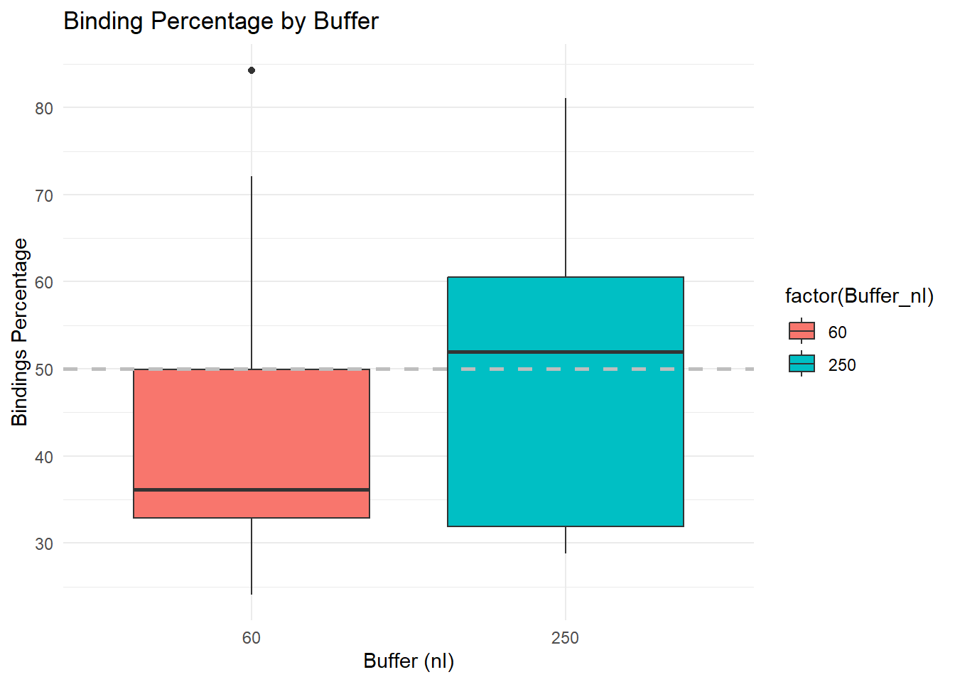

Past versions of unnamed-chunk-7-2.png

Version	Author	Date
b08a78b	Paloma	2024-10-16

# Boxplot of Binding Percentage vs Spike
ggplot(data, aes(x = factor(Spike), y = Binding.Perc, fill = Spike)) +
  geom_boxplot() +
  labs(title = "Binding Percentage by Spike",
       x = "Spike", y = "Binding Percentage") +
   scale_y_continuous(n.breaks = 10) +  
   geom_hline(yintercept = 50, linetype = "dashed", color = "gray", linewidth = 1) +
  theme_minimal()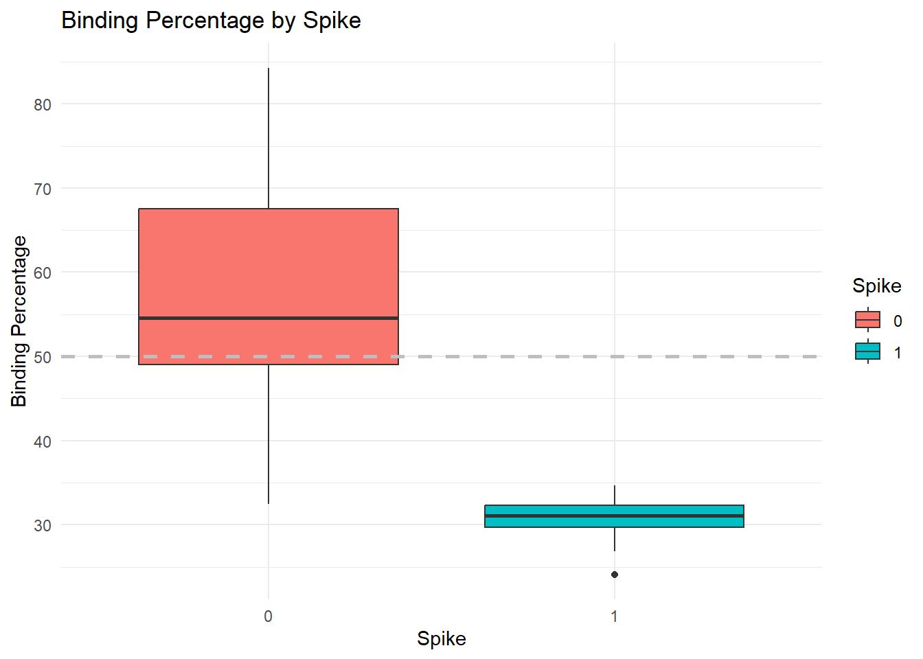

Past versions of unnamed-chunk-7-3.png

Version	Author	Date
b08a78b	Paloma	2024-10-16

Coef. of variation percentage

# Boxplot of CV Percentage vs Buffer & Spike
ggplot(data, aes(x = factor(Buffer_nl), y = CV.Perc, fill = factor(Spike))) +
  geom_boxplot() +
  labs(title = "Coef. of variation by Buffer and Spike",
       x = "Buffer (nl)", y = "Coef of variation %") +
   scale_y_continuous(n.breaks = 10) +  
  theme_minimal()

Past versions of unnamed-chunk-8-1.png

Version	Author	Date
b08a78b	Paloma	2024-10-16

Deviation from 50% binding

# Box plot to visualize distribution of Binding deviation by Buffer and Spike
ggplot(data, aes(x = factor(Buffer_nl), y = Binding_deviation, fill = factor(Spike))) +
  geom_boxplot() +
  labs(title = "Binding deviation by Buffer and Spike",
       x = "Buffer (nl)", y = "Binding deviation") +
   scale_y_continuous(n.breaks = 10) +  
  theme_minimal()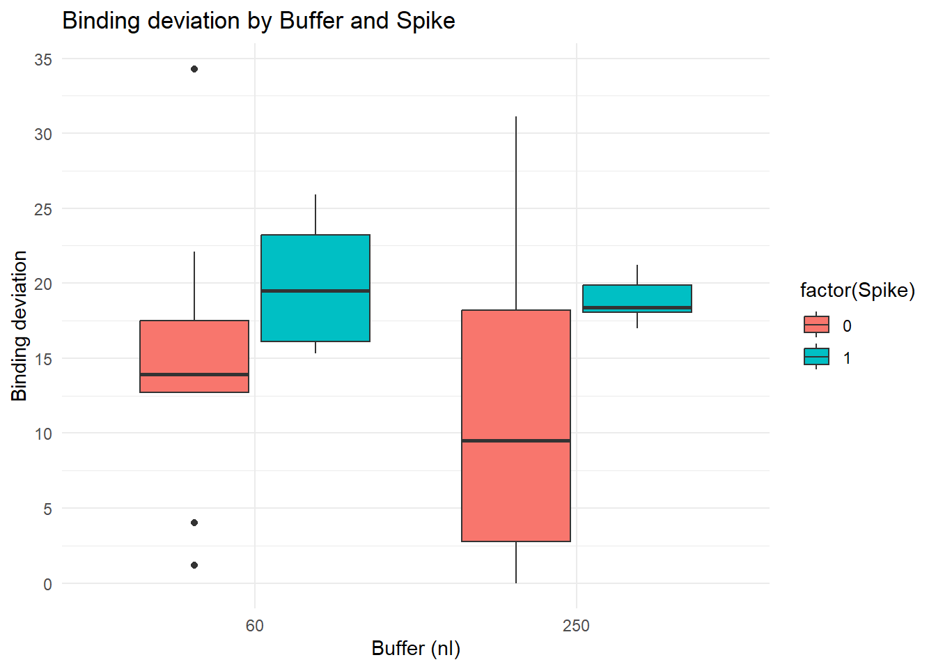

Past versions of unnamed-chunk-9-1.png

Version	Author	Date
b08a78b	Paloma	2024-10-16

wflow_publish(“./analysis/ELISA_visualizations.Rmd”)

wflow_status()

Session information

sessionInfo()

R version 4.1.0 (2021-05-18)
Platform: x86_64-w64-mingw32/x64 (64-bit)
Running under: Windows 10 x64 (build 19045)

Matrix products: default

locale:
[1] LC_COLLATE=English_United States.1252 
[2] LC_CTYPE=English_United States.1252   
[3] LC_MONETARY=English_United States.1252
[4] LC_NUMERIC=C                          
[5] LC_TIME=English_United States.1252    

attached base packages:
[1] stats     graphics  grDevices utils     datasets  methods   base     

other attached packages:
[1] RColorBrewer_1.1-3 ggplot2_3.5.1      knitr_1.48         dplyr_1.1.2       
[5] workflowr_1.7.1   

loaded via a namespace (and not attached):
 [1] tidyselect_1.2.0  xfun_0.47         bslib_0.8.0       splines_4.1.0    
 [5] lattice_0.20-44   colorspace_2.1-0  vctrs_0.6.5       generics_0.1.3   
 [9] htmltools_0.5.8.1 yaml_2.3.7        mgcv_1.8-35       utf8_1.2.3       
[13] rlang_1.1.0       jquerylib_0.1.4   later_1.3.0       pillar_1.9.0     
[17] glue_1.6.2        withr_3.0.1       lifecycle_1.0.4   stringr_1.5.1    
[21] munsell_0.5.1     gtable_0.3.5      evaluate_1.0.0    labeling_0.4.3   
[25] callr_3.7.6       fastmap_1.1.1     httpuv_1.6.9      ps_1.7.5         
[29] fansi_1.0.4       highr_0.11        Rcpp_1.0.10       promises_1.2.0.1 
[33] scales_1.3.0      cachem_1.0.7      jsonlite_1.8.9    farver_2.1.1     
[37] fs_1.5.2          digest_0.6.31     stringi_1.7.12    processx_3.8.1   
[41] getPass_0.2-2     rprojroot_2.0.4   grid_4.1.0        cli_3.6.1        
[45] tools_4.1.0       magrittr_2.0.3    sass_0.4.9        tibble_3.2.1     
[49] whisker_0.4.1     pkgconfig_2.0.3   Matrix_1.3-3      rmarkdown_2.28   
[53] httr_1.4.7        rstudioapi_0.16.0 R6_2.5.1          nlme_3.1-152     
[57] git2r_0.31.0      compiler_4.1.0