Uncovering Machine Learning’s Potential in Nowcasting GDP

Introduction

Collaborators

We have a team of people that consists of statisticians, econometricians and data scientists.

• Dawie van Lill 🗣️
• François Kamper
• Sebastian Krantz

📧 dvanlill@sun.ac.za

Research question(s)

There are two parts to our research question. One part relates to performance, the other to ease of use.

Do machine learning (and deep learning) methods contribute to forecasting performance over and above the traditional forecasting models? How easy are these methods to implement?

Managing expectations

This is not a technical talk on the methods used.

The talk is more about our results and the way that our experience translates to practitioners.

Please reach out

Contact us after the presentation to discuss model details. We would love to know how we can improve our models!

Contribution

Naive forecasting benchmark versus DFM, ML and DL

DFM and ML models

1. DFM (M)
2. SVR (M)
3. RF (M) **
4. GBM (M) **

MLP-based models

5. MLP (M)
6. N-BEATS (U & M)
7. N-HiTS (M)

U = Univariate, M = Multivariate, MLP = Multilayer Perceptron

Contribution

Naive forecasting benchmark versus DFM, ML and DL

RNN-based models

8. RNN (M)
9. RNN-LSTM (M)
10. RNN-GRU (M)
11. TCN (M)
12. DilatedRNN (M)

Transformer models

13. Temporal Fusion Transformer (U)
14. Informer (M)
15. Autoformer (M)

RNN = Recurrent neural network

Useful libraries

Data

Data

The target variable represents the seasonally adjusted, annualized quarter-on-quarter GDP growth rate from 1959Q2 to 2023Q2

Data for quarterly and monthly macroeconomic variables are gathered from the FRED-QD and FRED-MD databases, with suggested transformations applied.

Data preparation

Monthly vintage data is available, while GDP data is at a quarterly frequency, presenting a mixed frequency issue

To resolve this problem, we block the monthly data.

• This entails creating new variables from the values of the first, second, and third month of each quarter.

Dynamic factor models

Dynamic factor models

We employ a Mixed Frequency DFM per Bańbura and Modugno (2014) with 9 factors evolving in a global VAR(4)

We also use a blocked factor structure as in Bok et al. (2018) with 13 factors in 9 blocks, covering various economic sectors. The blocks and number of factors are presented below

global (2), output and income (1), labor market (1), consumption, orders, and inventories (2), housing (1), money and credit (2), interest and exchange rates (2), prices (1), and stock market (1).

Dynamic factor models

Finally, we estimate bridge-equation models with monthly DFMs using two methods:

1. Aggregating monthly factors to nowcast GDP via a linear model
2. Distributing monthly factors into various quarterly variables and applying LASSO for nowcasting

These bridge models allow for both global and blocked factor structures.

Our goal in using both mixed-frequency and bridge equation models is to assess potential gains from mixed-frequency in DFM estimation.

Machine learning models

Support vector regression

Support vector regression

In support vector regression (SVR) we fit a function from a reproducing kernel Hilbert space (RKHS) to the data via the epsilon (\(\epsilon\)) insensitive loss function.

The fit is regularized via the so-called cost parameter, to be selected via temporal cross-validation, and we set \(\epsilon = 1\) throughout.

We consider forming RKHS via the linear, radial basis and sigmoid kernels. The latter two kernels require specification of a hyper-parameter to be selected via temporal cross-validation.

Support vector regression

We found that including all the available predictive features in the fitting process to adversely effect results.To circumvent this, we applied a simple screening process to data from the training period only.

We only include variables with absolute correlation with the target (over the training period) exceeding a specified threshold. The threshold is chosen using temporal cross-validation.

Code

from matplotlib.ticker import MultipleLocator, AutoMinorLocator
from matplotlib.dates import YearLocator
import matplotlib.pyplot as plt
import pandas as pd

data = pd.read_csv('../presentation/01_data/tidy_svr.csv')

data['ds'] = pd.to_datetime(data['ds'])

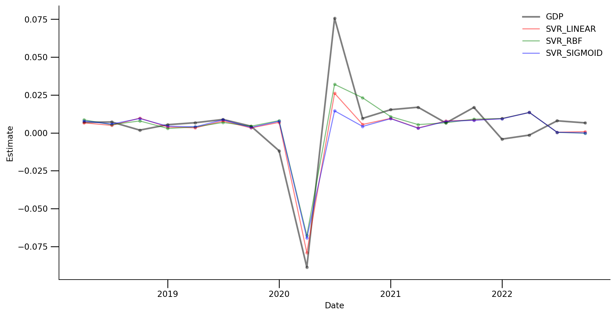
models_to_plot = ['SVR_LINEAR', 'SVR_RBF',
                  'SVR_SIGMOID', 'GDP']

filtered_data = data[data['Model'].isin(models_to_plot)]

grouped = filtered_data.groupby('Model')

selected_data = pd.concat([group.iloc[::3] for _, group in grouped])

model_color_dict = {
    'SVR_LINEAR': 'red',
    'SVR_RBF': 'green',
    'SVR_SIGMOID': 'blue',
    'GDP': 'black'
}


fig, ax = plt.subplots(figsize=(12, 6))

ax.xaxis.set_major_locator(YearLocator())

ax.spines['top'].set_visible(False)
ax.spines['right'].set_visible(False)

ax.tick_params(which="major", width=1.0)
ax.tick_params(which="major", length=10)
ax.tick_params(which="minor", width=1.0, labelsize=10)
ax.tick_params(which="minor", length=5, labelsize=10, labelcolor="0.25")

ax.set_ylabel("Estimate", weight="medium")
ax.set_xlabel("Date", weight="medium")

default_linewidth = 1.2
gdp_linewidth = 2

for model in selected_data['Model'].unique():
    subset = selected_data[selected_data['Model'] == model]
    ax.scatter(subset['ds'], subset['Estimate'], s=10, color=model_color_dict[model],
               edgecolor=model_color_dict[model], linewidth=1, zorder=-20, alpha=0.3)

    linewidth = gdp_linewidth if model == 'GDP' else default_linewidth
    ax.plot(subset['ds'], subset['Estimate'],
            c=model_color_dict[model], linewidth=linewidth, alpha=0.5, label=model)

ax.legend(frameon=False)

plt.show()

Figure 1: SVR models

MLP-based models

MLP-based models

We explore three types of MLP-based models:

1. Standard MLP
2. N-BEATS and N-BEATSx
3. N-HiTS

Both N-BEATS and N-HiTS utilize a learnable architecture to directly capture the historical data’s backward and forward-looking components.

Code

data = pd.read_csv('../presentation/01_data/tidy_results.csv')

data['ds'] = pd.to_datetime(data['ds'])

models_to_plot = ['AutoMLP', 'AutoNHITS',
                  'AutoNBEATS', 'AutoNBEATSx', 'GDP']

filtered_data = data[data['Model'].isin(models_to_plot)]

grouped = filtered_data.groupby('Model')

selected_data = pd.concat([group.iloc[::3] for _, group in grouped])

# Map models to colors
model_color_dict = {
    'AutoMLP': 'red',
    'AutoNHITS': 'green',
    'AutoNBEATS': 'blue',
    'AutoNBEATSx': 'cyan',
    'GDP': 'black'
}


fig, ax = plt.subplots(figsize=(12, 6))

ax.xaxis.set_major_locator(YearLocator())

ax.spines['top'].set_visible(False)
ax.spines['right'].set_visible(False)

ax.tick_params(which="major", width=1.0)
ax.tick_params(which="major", length=10)
ax.tick_params(which="minor", width=1.0, labelsize=10)
ax.tick_params(which="minor", length=5, labelsize=10, labelcolor="0.25")

ax.set_ylabel("Estimate", weight="medium")
ax.set_xlabel("Date", weight="medium")

default_linewidth = 1.2
gdp_linewidth = 2

for model in selected_data['Model'].unique():
    subset = selected_data[selected_data['Model'] == model]
    ax.scatter(subset['ds'], subset['Estimate'], s=10, color=model_color_dict[model],
               edgecolor=model_color_dict[model], linewidth=1, zorder=-20, alpha=0.3)

    linewidth = gdp_linewidth if model == 'GDP' else default_linewidth
    ax.plot(subset['ds'], subset['Estimate'],
            c=model_color_dict[model], linewidth=linewidth, alpha=0.5, label=model)

ax.legend(frameon=False)

plt.show()

Figure 2: MLP models

RNN-based models

RNN-based models

We examine five types of RNN-based models:

1. Standard RNN
2. RNN with LSTM
3. RNN with GRU
4. TCN
5. Dilated RNN

This class of model is our top performer among deep learning models.

RNN-based models

LSTM and GRU leverage gating mechanisms, distinguishing them from standard RNNs by addressing the vanishing gradient issue and facilitating long-term dependency capture.

Dilated RNN employs time dilation (skipped steps) for efficient long-sequence capture without parameter increase.

TCNs, on the other hand, utilize dilated causal convolutions, offering efficient long-term dependency management and enhanced parallelism.

Code

data = pd.read_csv('../presentation/01_data/tidy_results.csv')

data['ds'] = pd.to_datetime(data['ds'])

models_to_plot = ['AutoDilatedRNN', 'AutoGRU',
                  'AutoRNN', 'AutoTCN', 'AutoLSTM', 'GDP']

filtered_data = data[data['Model'].isin(models_to_plot)]

grouped = filtered_data.groupby('Model')

selected_data = pd.concat([group.iloc[::3] for _, group in grouped])

# Map models to colors
model_color_dict = {
    'AutoDilatedRNN': 'red',
    'AutoGRU': 'green',
    'AutoRNN': 'blue',
    'AutoTCN': 'cyan',
    'AutoLSTM': 'purple',
    'GDP': 'black'
}


fig, ax = plt.subplots(figsize=(12, 6))

ax.xaxis.set_major_locator(YearLocator())

ax.spines['top'].set_visible(False)
ax.spines['right'].set_visible(False)

ax.tick_params(which="major", width=1.0)
ax.tick_params(which="major", length=10)
ax.tick_params(which="minor", width=1.0, labelsize=10)
ax.tick_params(which="minor", length=5, labelsize=10, labelcolor="0.25")

ax.set_ylabel("Estimate", weight="medium")
ax.set_xlabel("Date", weight="medium")

default_linewidth = 1.2
gdp_linewidth = 2

for model in selected_data['Model'].unique():
    subset = selected_data[selected_data['Model'] == model]
    ax.scatter(subset['ds'], subset['Estimate'], s=10, color=model_color_dict[model],
               edgecolor=model_color_dict[model], linewidth=1, zorder=-20, alpha=0.3)

    linewidth = gdp_linewidth if model == 'GDP' else default_linewidth
    ax.plot(subset['ds'], subset['Estimate'],
            c=model_color_dict[model], linewidth=linewidth, alpha=0.5, label=model)

ax.legend(frameon=False)

plt.show()

Figure 3: RNN models

Transformer models

Transformer models

We examine three transformer-based models:

1. Temporal Fusion Transformer
2. Informer
3. Autoformer

These models, unlike RNNs, utilize self-attention, enhancing dependency management and parallel processing.

Despite this, their high computational demands, large dataset requirements, and difficulty with sequential data may limit their time series forecasting efficacy.

Code

data = pd.read_csv('../presentation/01_data/tidy_results.csv')

data['ds'] = pd.to_datetime(data['ds'])

models_to_plot = ['AutoTFT', 'AutoInformer',
                  'AutoAutoformer', 'GDP']

filtered_data = data[data['Model'].isin(models_to_plot)]

# Group by model and select every third row
grouped = filtered_data.groupby('Model')

selected_data = pd.concat([group.iloc[::3] for _, group in grouped])

# Map models to colors
model_color_dict = {
    'AutoTFT': 'red',
    'AutoInformer': 'green',
    'AutoAutoformer': 'blue',
    'GDP': 'black'
}


fig, ax = plt.subplots(figsize=(12, 6))

ax.xaxis.set_major_locator(YearLocator())

ax.spines['top'].set_visible(False)
ax.spines['right'].set_visible(False)

ax.tick_params(which="major", width=1.0)
ax.tick_params(which="major", length=10)
ax.tick_params(which="minor", width=1.0, labelsize=10)
ax.tick_params(which="minor", length=5, labelsize=10, labelcolor="0.25")

ax.set_ylabel("Estimate", weight="medium")
ax.set_xlabel("Date", weight="medium")

default_linewidth = 1.2
gdp_linewidth = 2

for model in selected_data['Model'].unique():
    subset = selected_data[selected_data['Model'] == model]
    ax.scatter(subset['ds'], subset['Estimate'], s=10, color=model_color_dict[model],
               edgecolor=model_color_dict[model], linewidth=1, zorder=-20, alpha=0.3)

    linewidth = gdp_linewidth if model == 'GDP' else default_linewidth
    ax.plot(subset['ds'], subset['Estimate'],
            c=model_color_dict[model], linewidth=linewidth, alpha=0.5, label=model)

ax.legend(frameon=False)

plt.show()

Figure 4: Transformer models

Results

Model Performance: Average Monthly Nowcast, Sorted by RMSE

	Bias	RMSE	MAE	MAPE	U2	Bias Prop.	Var. Prop.	Cov. Prop.
DilatedRNN	0.43	0.86	0.61	107.59	0.54	0.25	0.16	0.59
LSTM	0.40	0.89	0.59	100.75	0.52	0.20	0.24	0.55
RNN	0.41	0.93	0.61	101.24	0.55	0.20	0.24	0.56
GRU	0.46	1.02	0.67	114.39	0.61	0.21	0.35	0.44
DFM Global	-0.14	1.02	0.71	115.06	0.72	0.02	0.02	0.96
SVR Linear	-0.10	1.15	0.74	121.20	0.70	0.01	0.27	0.72
SVR Sigmoid	-0.08	1.25	0.81	108.77	0.68	0.00	0.47	0.53
DFM Blocked	-0.15	1.34	0.79	117.14	0.58	0.01	0.02	0.97
SVR RBF	0.15	1.35	0.92	127.70	0.76	0.01	0.71	0.28
DFM_lasso_global	-0.16	1.44	0.80	92.40	0.51	0.01	0.31	0.68
DFM_lasso_blocked	-0.18	1.61	0.81	109.57	0.55	0.01	0.08	0.91
DFM_lm_global	-0.45	1.66	1.11	132.48	0.77	0.07	0.08	0.85
DFM_lm_blocked	-0.31	1.68	0.87	98.37	0.63	0.03	0.02	0.95
TCN	0.52	1.99	0.99	113.40	0.78	0.07	0.75	0.18
Informer	0.15	2.99	1.43	112.38	0.97	0.00	0.68	0.32
TFT	0.07	3.03	1.41	96.10	0.87	0.00	0.54	0.46
NBEATS	0.12	3.05	1.69	158.31	0.93	0.00	0.29	0.71
NHITS	0.14	3.33	1.86	154.64	0.97	0.00	0.04	0.96
NBEATSx	-0.03	3.85	2.19	172.27	1.04	0.00	0.01	0.99
MLP	0.08	4.09	2.03	139.90	0.98	0.00	0.01	0.99
Naive	0.00	4.62	2.24	152.15	1.00	0.00	0.00	1.00
Autoformer	-2.59	10.49	4.27	501.43	7.52	0.06	0.42	0.52

Model Performance: Final Month of Quarter, Sorted by RMSE

	Bias	RMSE	MAE	MAPE	U2	Bias Prop.	Var. Prop.	Cov. Prop.
DFM Global	0.12	0.74	0.54	106.35	0.59	0.03	0.09	0.88
DFM_lm_global	0.21	0.79	0.54	90.45	0.48	0.07	0.04	0.89
DFM Blocked	0.15	0.84	0.59	115.70	0.54	0.03	0.07	0.90
RNN	0.24	0.86	0.56	83.97	0.41	0.08	0.58	0.34
DilatedRNN	0.34	0.88	0.64	84.65	0.41	0.15	0.31	0.54
SVR Sigmoid	0.04	0.88	0.62	80.97	0.60	0.00	0.43	0.57
SVR Linear	0.01	0.93	0.60	108.01	0.64	0.00	0.19	0.81
GRU	0.25	1.06	0.74	97.64	0.50	0.06	0.67	0.28
TCN	0.36	1.07	0.65	95.19	0.51	0.11	0.43	0.46
LSTM	0.29	1.13	0.64	74.43	0.45	0.06	0.67	0.26
SVR RBF	0.30	1.46	0.88	119.53	0.75	0.04	0.76	0.20
DFM_lm_blocked	-0.09	1.51	0.90	78.04	0.65	0.00	0.41	0.58
DFM_lasso_blocked	0.32	1.94	1.02	101.59	0.69	0.03	0.80	0.17
DFM_lasso_global	0.05	2.02	1.06	98.01	0.61	0.00	0.67	0.33
Informer	0.20	3.01	1.37	95.55	1.00	0.00	0.65	0.35
TFT	0.00	3.13	1.47	105.24	0.86	0.00	0.44	0.56
NBEATS	0.21	3.21	1.89	184.95	2.31	0.00	0.17	0.83
NHITS	0.37	3.36	1.90	160.45	0.92	0.01	0.02	0.97
MLP	0.13	3.67	1.98	143.29	1.00	0.00	0.05	0.95
NBEATSx	-0.05	3.91	2.20	178.69	1.04	0.00	0.00	1.00
Naive	0.00	4.62	2.24	152.15	1.00	0.00	0.00	1.00
Autoformer	-7.59	29.83	9.35	1202.56	22.44	0.06	0.75	0.19

Conclusion

Conclusion

DFMs, RNN-based models and SVRs do the best in terms of nowcasting performance.

Newer MLP and transformer based models do markedly worse.

The latter class of models take the longest to tune. Computational cost is high.

Our prediction is that these models will become valuable in future, but greater investment required in trying to understand how they apply to time series forecasting.

References

Bańbura, Marta, and Michele Modugno. 2014. “Maximum Likelihood Estimation of Factor Models on Datasets with Arbitrary Pattern of Missing Data.” Journal of Applied Econometrics 29 (1): 133–60.

Bok, Brandyn, Daniele Caratelli, Domenico Giannone, Argia M Sbordone, and Andrea Tambalotti. 2018. “Macroeconomic Nowcasting and Forecasting with Big Data.” Annual Review of Economics 10: 615–43.