Enrichment Analysis
Steve Pederson
26 January, 2020
Last updated: 2020-01-26
Checks: 6 1
Knit directory: 20170327_Psen2S4Ter_RNASeq/
This reproducible R Markdown analysis was created with workflowr (version 1.6.0). The Checks tab describes the reproducibility checks that were applied when the results were created. The Past versions tab lists the development history.
The R Markdown file has unstaged changes. To know which version of the R Markdown file created these results, you’ll want to first commit it to the Git repo. If you’re still working on the analysis, you can ignore this warning. When you’re finished, you can run wflow_publish to commit the R Markdown file and build the HTML.
Great job! The global environment was empty. Objects defined in the global environment can affect the analysis in your R Markdown file in unknown ways. For reproduciblity it’s best to always run the code in an empty environment.
The command set.seed(20200119) was run prior to running the code in the R Markdown file. Setting a seed ensures that any results that rely on randomness, e.g. subsampling or permutations, are reproducible.
Great job! Recording the operating system, R version, and package versions is critical for reproducibility.
Nice! There were no cached chunks for this analysis, so you can be confident that you successfully produced the results during this run.
Great job! Using relative paths to the files within your workflowr project makes it easier to run your code on other machines.
Great! You are using Git for version control. Tracking code development and connecting the code version to the results is critical for reproducibility. The version displayed above was the version of the Git repository at the time these results were generated.
Note that you need to be careful to ensure that all relevant files for the analysis have been committed to Git prior to generating the results (you can use wflow_publish or wflow_git_commit). workflowr only checks the R Markdown file, but you know if there are other scripts or data files that it depends on. Below is the status of the Git repository when the results were generated:
Ignored files:
    Ignored:    .Rhistory
    Ignored:    .Rproj.user/

Untracked files:
    Untracked:  analysis/figure/

Unstaged changes:
    Modified:   analysis/3_Enrichment.Rmd
Note that any generated files, e.g. HTML, png, CSS, etc., are not included in this status report because it is ok for generated content to have uncommitted changes.
These are the previous versions of the R Markdown and HTML files. If you’ve configured a remote Git repository (see ?wflow_git_remote), click on the hyperlinks in the table below to view them.
| File | Version | Author | Date | Message |
|---|---|---|---|---|
| Rmd | ba189be | Steve Ped | 2020-01-26 | Corrected packages |
| Rmd | 68033fe | Steve Ped | 2020-01-26 | Corrected chunk labels after publishing DE analysis |
| Rmd | 25922d6 | Steve Ped | 2020-01-26 | Added first pass of enrichment |
Setup
library(tidyverse)
library(magrittr)
library(edgeR)
library(scales)
library(pander)
library(goseq)
library(msigdbr)
library(AnnotationDbi)
library(RColorBrewer)
theme_set(theme_bw())
panderOptions("table.split.table", Inf)
panderOptions("table.style", "rmarkdown")
panderOptions("big.mark", ",")samples <- read_csv("data/samples.csv") %>%
distinct(sampleName, .keep_all = TRUE) %>%
dplyr::select(sample = sampleName, sampleID, genotype) %>%
mutate(
genotype = factor(genotype, levels = c("WT", "Het", "Hom")),
mutant = genotype %in% c("Het", "Hom"),
homozygous = genotype == "Hom"
)
genoCols <- samples$genotype %>%
levels() %>%
length() %>%
brewer.pal("Set1") %>%
setNames(levels(samples$genotype))dgeList <- read_rds("data/dgeList.rds")
fit <- read_rds("data/fit.rds")
entrezGenes <- dgeList$genes %>%
dplyr::filter(!is.na(entrezid)) %>%
unnest(entrezid) %>%
dplyr::rename(entrez_gene = entrezid)formatP <- function(p, m = 0.0001){
out <- rep("", length(p))
out[p < m] <- sprintf("%.2e", p[p<m])
out[p >= m] <- sprintf("%.4f", p[p>=m])
out
}Introduction
Enrichment analysis for this datast present some challenges. Despite normalisation to account for gene length and GC bias, some appeared to still be present in the final results. In addition, the confounding of incomplete rRNA removal with genotype may lead to other distortions in both DE genes and ranking statistics.
Two methods for enrichment analysis will be undertaken.
- Testing for enrichment within discrete sets of DE genes as defined in the previous steps
- Testing for enrichment within ranked lists, regardless of DE status or statistical significance.
Testing for enrichment within discrete gene sets will be performed using goseq as this allows for the incorporation of a single covariate as a predictor of differential expression. GC content, gene length and correlation with rRNA removal can all be supplied as separate covariates.
Testing for enrichment with ranked lists will be performed using fry as this can take a dgeList directly. However, in order for testing to be robust in the context of bias, normalised counts after CQN will be used for generation of a new dgeList for testing.
Databases used for testing
Data was sourced using the msigdbr package. The initial database used for testing was the Hallmark Gene Sets, with mappings from gene-set to EntrezGene IDs performed by the package authors.
Discrete DE Gene Sets
topTables <- list.files(
    path = "output", pattern = "Vs.+csv", full.names = TRUE
) %>%
    sapply(read_csv, simplify = FALSE) %>%
    set_names(basename(names(.))) %>%
    set_names(str_remove(names(.), ".csv")) %>%
    lapply(function(x){
        x %>%
            mutate(
                entrezid = dgeList$genes$entrezid[gene_id]
            )
    })
Effects of the *psen2S4Ter mutation
The first step of analysis using goseq, regardless of the geneset, is estimation of the probability weight function (PWF) which quantifies the probablity of a gene being considered as DE based on a single covariate. Two possible covariates (GC content & Gene Length) were checked
pwf <- c("gc_content", "length") %>%
    sapply(
        function(x){
            topTables$psen2VsWT %>%
                dplyr::select(gene_id, DE, covariate = one_of(x)) %>%
                distinct(gene_id, .keep_all = TRUE) %>%
                with(
                    nullp(
                        DEgenes = structure(
                            as.integer(DE), names = gene_id
                        ),
                        genome = "danRer10",
                        id = "ensGene",
                        bias.data = covariate,
                        plot.fit = FALSE
                    )
                )
        },
        simplify = FALSE
    )
par(mfrow = c(1, length(pwf)))
names(pwf) %>%
lapply(function(x){
plotPWF(pwf[[x]], main = x)
})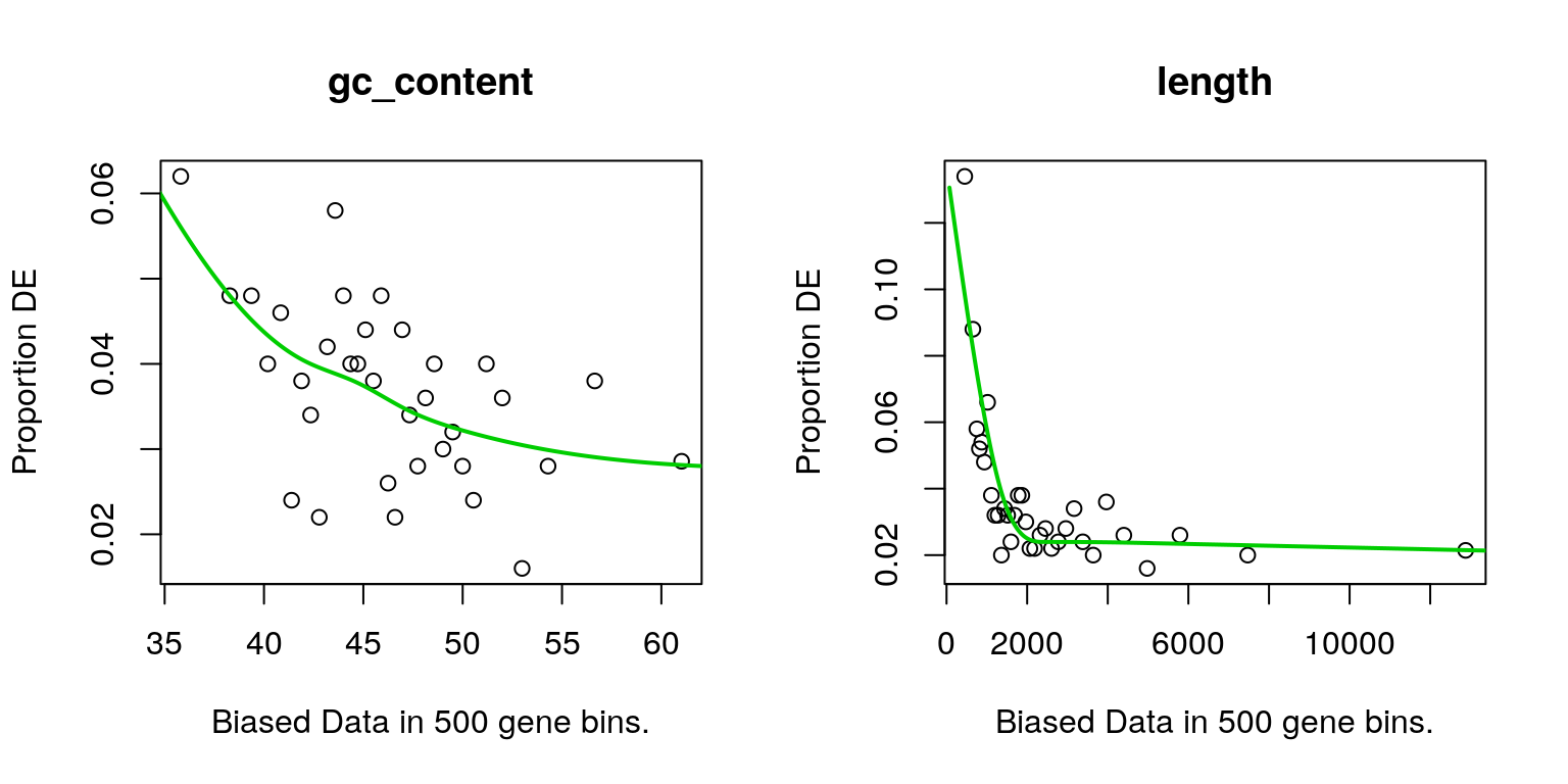
Bias data based on each of the possible covariates. Both appeared to impact the probability of a gene being DE to some extent, with gene length being selected as the covariate for usage inthe goseq model.
[[1]]
NULL

[[2]]
NULL
par(mfrow = c(1, 1))Hallmark Gene Sets
hm <- msigdbr("Danio rerio", category = "H")  %>%
  left_join(entrezGenes) %>%
  dplyr::filter(!is.na(gene_id))
hmByGene <- hm %>%
split(f = .$gene_id) %>%
lapply(extract2, "gs_name")Mappings are required from gene to pathway, and Ensembl identifiers were used to map from gene to pathway, based on the mappings in the previously used annotations (Ensembl Release 96). A total of 3459 Ensembl IDs were mapped to pathways from the hallmark gene sets. This contrasts with 3458 EntrezGene IDs.
hmGoseq <- goseq(pwf$length, gene2cat = hmByGene) %>%
    as_tibble %>%
  dplyr::filter(numDEInCat > 0) %>%
  mutate(
    adjP = p.adjust(over_represented_pvalue, method = "bonf"),
    FDR = p.adjust(over_represented_pvalue, method = "fdr")
  ) %>%
  dplyr::select(-contains("under"))
No hallmark genesets were considered to be enriched after adjusting for the observed length bias in the data.
KEGG Gene Sets
The same mapping process was applied to KEGG gene sets.
kg <- msigdbr("Danio rerio", category = "C2", subcategory = "CP:KEGG")  %>%
  left_join(entrezGenes) %>%
  dplyr::filter(!is.na(gene_id))
kgByGene <- kg %>%
split(f = .$gene_id) %>%
lapply(extract2, "gs_name")A total of 3614 Ensembl IDs were mapped to pathways from the KEGG gene sets. This contrasts with 3603 EntrezGene IDs.
kgGoseq <- goseq(pwf$length, gene2cat = kgByGene) %>%
  as_tibble %>%
  dplyr::filter(numDEInCat > 0) %>%
  mutate(
    adjP = p.adjust(over_represented_pvalue, method = "bonf"),
    FDR = p.adjust(over_represented_pvalue, method = "fdr")
  ) %>%
  dplyr::select(-contains("under"))
kgGoseq %>%
dplyr::slice(1:5) %>%
dplyr::rename(p = over_represented_pvalue) %>%
mutate(
p = formatP(p),
adjP = formatP(adjP),
FDR = formatP(FDR)
) %>%
dplyr::select(
Category = category,
DE = numDEInCat,
`Set Size` = numInCat,
p,
`p~bonf~` = adjP,
`p~FDR~` = FDR
) %>%
pander(
justify = "lrrrrr",
caption = paste(
"The", nrow(.), "most highly-ranked KEGG pathways.",
"Bonferroni-adjusted p-values are the most stringent and give high",
"confidence when below 0.05."
)
)| Category | DE | Set Size | p | pbonf | pFDR |
|---|---|---|---|---|---|
| KEGG_RIBOSOME | 26 | 80 | 4.65e-12 | 5.20e-10 | 5.20e-10 |
| KEGG_OXIDATIVE_PHOSPHORYLATION | 14 | 119 | 0.0070 | 0.7892 | 0.3086 |
| KEGG_CYSTEINE_AND_METHIONINE_METABOLISM | 4 | 26 | 0.0101 | 1.0000 | 0.3086 |
| KEGG_PARKINSONS_DISEASE | 13 | 112 | 0.0118 | 1.0000 | 0.3086 |
| KEGG_HUNTINGTONS_DISEASE | 15 | 159 | 0.0138 | 1.0000 | 0.3086 |
Notably, the KEGG gene-set for Ribosomal genes was detected as enriched. This is likely to be due to the previosuly discussed contaminant.
GO Gene Sets
The same mapping process was applied to GO gene sets.
goSummaries <- url("https://uofabioinformaticshub.github.io/summaries2GO/data/goSummaries.RDS") %>%
  readRDS() %>%
  mutate(
    Term = Term(id),
    gs_name = Term %>% str_to_upper() %>% str_replace_all("[ -]", "_"),
    gs_name = paste0("GO_", gs_name)
    )
go <- msigdbr("Danio rerio", category = "C5") %>%
left_join(entrezGenes) %>%
dplyr::filter(!is.na(gene_id)) minPath <- 3
goByGene <- go %>%
left_join(goSummaries) %>%
dplyr::filter(shortest_path >= minPath) %>%
split(f = .$gene_id) %>%
lapply(extract2, "gs_name")A total of 11245 Ensembl IDs were mapped to pathways from the GO gene sets. This contrasts with 11359 EntrezGene IDs. In addition GO genesets were restricted to those with 3 or more steps back to each ontology root.
goGoseq <- goseq(pwf$length, gene2cat = goByGene) %>%
  as_tibble %>%
  dplyr::filter(numDEInCat > 0) %>%
  mutate(
    adjP = p.adjust(over_represented_pvalue, method = "bonf"),
    FDR = p.adjust(over_represented_pvalue, method = "fdr")
  ) %>%
  dplyr::select(-contains("under"))
goGoseq %>%
dplyr::filter(adjP < 0.05) %>%
dplyr::rename(p = over_represented_pvalue) %>%
mutate(
p = formatP(p),
adjP = formatP(adjP),
FDR = formatP(FDR)
) %>%
dplyr::select(
Category = category,
DE = numDEInCat,
`Set Size` = numInCat,
p,
`p~bonf~` = adjP,
`p~FDR~` = FDR
) %>%
pander(
justify = "lrrrrr",
caption = paste(
"The", nrow(.), "most highly-ranked GO terms.",
"Bonferroni-adjusted p-values are the most stringent and give high",
"confidence when below 0.05, and all terms reached this threshold.",
"However, most terms indicate the presence of rRNA once again."
)
)| Category | DE | Set Size | p | pbonf | pFDR |
|---|---|---|---|---|---|
| GO_COTRANSLATIONAL_PROTEIN_TARGETING_TO_MEMBRANE | 28 | 93 | 2.42e-13 | 9.33e-10 | 9.33e-10 |
| GO_CYTOSOLIC_RIBOSOME | 27 | 97 | 3.74e-12 | 1.44e-08 | 7.19e-09 |
| GO_ESTABLISHMENT_OF_PROTEIN_LOCALIZATION_TO_ENDOPLASMIC_RETICULUM | 27 | 105 | 1.17e-11 | 4.50e-08 | 1.50e-08 |
| GO_PROTEIN_TARGETING_TO_MEMBRANE | 30 | 171 | 1.67e-10 | 6.43e-07 | 1.55e-07 |
| GO_PROTEIN_LOCALIZATION_TO_ENDOPLASMIC_RETICULUM | 27 | 128 | 2.01e-10 | 7.74e-07 | 1.55e-07 |
| GO_NUCLEAR_TRANSCRIBED_MRNA_CATABOLIC_PROCESS | 30 | 183 | 1.03e-09 | 3.97e-06 | 6.62e-07 |
| GO_VIRAL_GENE_EXPRESSION | 29 | 172 | 1.59e-09 | 6.12e-06 | 8.74e-07 |
| GO_TRANSLATIONAL_INITIATION | 29 | 177 | 4.88e-09 | 1.88e-05 | 2.35e-06 |
| GO_CYTOSOLIC_PART | 30 | 206 | 8.07e-09 | 3.10e-05 | 3.45e-06 |
| GO_RNA_BINDING | 88 | 1,408 | 4.79e-08 | 0.0002 | 1.84e-05 |
| GO_CYTOSOLIC_LARGE_RIBOSOMAL_SUBUNIT | 15 | 51 | 1.26e-07 | 0.0005 | 4.40e-05 |
| GO_RIBOSOMAL_SUBUNIT | 28 | 175 | 3.31e-07 | 0.0013 | 0.0001 |
| GO_RIBOSOME | 30 | 210 | 3.83e-07 | 0.0015 | 0.0001 |
| GO_RNA_CATABOLIC_PROCESS | 34 | 337 | 7.18e-07 | 0.0028 | 0.0002 |
| GO_ESTABLISHMENT_OF_PROTEIN_LOCALIZATION_TO_MEMBRANE | 30 | 287 | 1.69e-06 | 0.0065 | 0.0004 |
| GO_ORGANIC_CYCLIC_COMPOUND_CATABOLIC_PROCESS | 40 | 474 | 1.82e-06 | 0.0070 | 0.0004 |
| GO_PROTEIN_TARGETING | 34 | 379 | 7.10e-06 | 0.0273 | 0.0016 |
| GO_ESTABLISHMENT_OF_PROTEIN_LOCALIZATION_TO_ORGANELLE | 38 | 484 | 9.76e-06 | 0.0376 | 0.0021 |
Effects of Homozygous Vs Heterozygous mutants
As only a small number of genes were detected as being classified as DE for this comparison, no testing was performed on this as a discrete set of DE genes.
devtools::session_info()─ Session info ───────────────────────────────────────────────────────────────
setting value
version R version 3.6.2 (2019-12-12)
os Ubuntu 18.04.3 LTS
system x86_64, linux-gnu
ui X11
language en_AU:en
collate en_AU.UTF-8
ctype en_AU.UTF-8
tz Australia/Adelaide
date 2020-01-26
─ Packages ───────────────────────────────────────────────────────────────────
package * version date lib source
AnnotationDbi * 1.48.0 2019-10-29 [2] Bioconductor
askpass 1.1 2019-01-13 [2] CRAN (R 3.6.0)
assertthat 0.2.1 2019-03-21 [2] CRAN (R 3.6.0)
backports 1.1.5 2019-10-02 [2] CRAN (R 3.6.1)
BiasedUrn * 1.07 2015-12-28 [2] CRAN (R 3.6.1)
Biobase * 2.46.0 2019-10-29 [2] Bioconductor
BiocFileCache 1.10.2 2019-11-08 [2] Bioconductor
BiocGenerics * 0.32.0 2019-10-29 [2] Bioconductor
BiocParallel 1.20.1 2019-12-21 [2] Bioconductor
biomaRt 2.42.0 2019-10-29 [2] Bioconductor
Biostrings 2.54.0 2019-10-29 [2] Bioconductor
bit 1.1-15.1 2020-01-14 [2] CRAN (R 3.6.2)
bit64 0.9-7 2017-05-08 [2] CRAN (R 3.6.0)
bitops 1.0-6 2013-08-17 [2] CRAN (R 3.6.0)
blob 1.2.1 2020-01-20 [2] CRAN (R 3.6.2)
broom 0.5.3 2019-12-14 [2] CRAN (R 3.6.2)
callr 3.4.0 2019-12-09 [2] CRAN (R 3.6.2)
cellranger 1.1.0 2016-07-27 [2] CRAN (R 3.6.0)
cli 2.0.1 2020-01-08 [2] CRAN (R 3.6.2)
colorspace 1.4-1 2019-03-18 [2] CRAN (R 3.6.0)
crayon 1.3.4 2017-09-16 [2] CRAN (R 3.6.0)
curl 4.3 2019-12-02 [2] CRAN (R 3.6.2)
DBI 1.1.0 2019-12-15 [2] CRAN (R 3.6.2)
dbplyr 1.4.2 2019-06-17 [2] CRAN (R 3.6.0)
DelayedArray 0.12.2 2020-01-06 [2] Bioconductor
desc 1.2.0 2018-05-01 [2] CRAN (R 3.6.0)
devtools 2.2.1 2019-09-24 [2] CRAN (R 3.6.1)
digest 0.6.23 2019-11-23 [2] CRAN (R 3.6.1)
dplyr * 0.8.3 2019-07-04 [2] CRAN (R 3.6.1)
edgeR * 3.28.0 2019-10-29 [2] Bioconductor
ellipsis 0.3.0 2019-09-20 [2] CRAN (R 3.6.1)
evaluate 0.14 2019-05-28 [2] CRAN (R 3.6.0)
fansi 0.4.1 2020-01-08 [2] CRAN (R 3.6.2)
forcats * 0.4.0 2019-02-17 [2] CRAN (R 3.6.0)
fs 1.3.1 2019-05-06 [2] CRAN (R 3.6.0)
geneLenDataBase * 1.22.0 2019-11-05 [2] Bioconductor
generics 0.0.2 2018-11-29 [2] CRAN (R 3.6.0)
GenomeInfoDb 1.22.0 2019-10-29 [2] Bioconductor
GenomeInfoDbData 1.2.2 2019-11-21 [2] Bioconductor
GenomicAlignments 1.22.1 2019-11-12 [2] Bioconductor
GenomicFeatures 1.38.1 2020-01-22 [2] Bioconductor
GenomicRanges 1.38.0 2019-10-29 [2] Bioconductor
ggplot2 * 3.2.1 2019-08-10 [2] CRAN (R 3.6.1)
git2r 0.26.1 2019-06-29 [2] CRAN (R 3.6.1)
glue 1.3.1 2019-03-12 [2] CRAN (R 3.6.0)
GO.db 3.10.0 2019-11-21 [2] Bioconductor
goseq * 1.38.0 2019-10-29 [2] Bioconductor
gtable 0.3.0 2019-03-25 [2] CRAN (R 3.6.0)
haven 2.2.0 2019-11-08 [2] CRAN (R 3.6.1)
highr 0.8 2019-03-20 [2] CRAN (R 3.6.0)
hms 0.5.3 2020-01-08 [2] CRAN (R 3.6.2)
htmltools 0.4.0 2019-10-04 [2] CRAN (R 3.6.1)
httpuv 1.5.2 2019-09-11 [2] CRAN (R 3.6.1)
httr 1.4.1 2019-08-05 [2] CRAN (R 3.6.1)
IRanges * 2.20.2 2020-01-13 [2] Bioconductor
jsonlite 1.6 2018-12-07 [2] CRAN (R 3.6.0)
knitr 1.27 2020-01-16 [2] CRAN (R 3.6.2)
later 1.0.0 2019-10-04 [2] CRAN (R 3.6.1)
lattice 0.20-38 2018-11-04 [4] CRAN (R 3.6.0)
lazyeval 0.2.2 2019-03-15 [2] CRAN (R 3.6.0)
lifecycle 0.1.0 2019-08-01 [2] CRAN (R 3.6.1)
limma * 3.42.0 2019-10-29 [2] Bioconductor
locfit 1.5-9.1 2013-04-20 [2] CRAN (R 3.6.0)
lubridate 1.7.4 2018-04-11 [2] CRAN (R 3.6.0)
magrittr * 1.5 2014-11-22 [2] CRAN (R 3.6.0)
Matrix 1.2-18 2019-11-27 [2] CRAN (R 3.6.1)
matrixStats 0.55.0 2019-09-07 [2] CRAN (R 3.6.1)
memoise 1.1.0 2017-04-21 [2] CRAN (R 3.6.0)
mgcv 1.8-31 2019-11-09 [4] CRAN (R 3.6.1)
modelr 0.1.5 2019-08-08 [2] CRAN (R 3.6.1)
msigdbr * 7.0.1 2019-09-04 [2] CRAN (R 3.6.2)
munsell 0.5.0 2018-06-12 [2] CRAN (R 3.6.0)
nlme 3.1-143 2019-12-10 [4] CRAN (R 3.6.2)
openssl 1.4.1 2019-07-18 [2] CRAN (R 3.6.1)
pander * 0.6.3 2018-11-06 [2] CRAN (R 3.6.0)
pillar 1.4.3 2019-12-20 [2] CRAN (R 3.6.2)
pkgbuild 1.0.6 2019-10-09 [2] CRAN (R 3.6.1)
pkgconfig 2.0.3 2019-09-22 [2] CRAN (R 3.6.1)
pkgload 1.0.2 2018-10-29 [2] CRAN (R 3.6.0)
prettyunits 1.1.1 2020-01-24 [2] CRAN (R 3.6.2)
processx 3.4.1 2019-07-18 [2] CRAN (R 3.6.1)
progress 1.2.2 2019-05-16 [2] CRAN (R 3.6.0)
promises 1.1.0 2019-10-04 [2] CRAN (R 3.6.1)
ps 1.3.0 2018-12-21 [2] CRAN (R 3.6.0)
purrr * 0.3.3 2019-10-18 [2] CRAN (R 3.6.1)
R6 2.4.1 2019-11-12 [2] CRAN (R 3.6.1)
rappdirs 0.3.1 2016-03-28 [2] CRAN (R 3.6.0)
RColorBrewer * 1.1-2 2014-12-07 [2] CRAN (R 3.6.0)
Rcpp 1.0.3 2019-11-08 [2] CRAN (R 3.6.1)
RCurl 1.98-1.1 2020-01-19 [2] CRAN (R 3.6.2)
readr * 1.3.1 2018-12-21 [2] CRAN (R 3.6.0)
readxl 1.3.1 2019-03-13 [2] CRAN (R 3.6.0)
remotes 2.1.0 2019-06-24 [2] CRAN (R 3.6.0)
reprex 0.3.0 2019-05-16 [2] CRAN (R 3.6.0)
rlang 0.4.2 2019-11-23 [2] CRAN (R 3.6.1)
rmarkdown 2.1 2020-01-20 [2] CRAN (R 3.6.2)
rprojroot 1.3-2 2018-01-03 [2] CRAN (R 3.6.0)
Rsamtools 2.2.1 2019-11-06 [2] Bioconductor
RSQLite 2.2.0 2020-01-07 [2] CRAN (R 3.6.2)
rstudioapi 0.10 2019-03-19 [2] CRAN (R 3.6.0)
rtracklayer 1.46.0 2019-10-29 [2] Bioconductor
rvest 0.3.5 2019-11-08 [2] CRAN (R 3.6.1)
S4Vectors * 0.24.3 2020-01-18 [2] Bioconductor
scales * 1.1.0 2019-11-18 [2] CRAN (R 3.6.1)
sessioninfo 1.1.1 2018-11-05 [2] CRAN (R 3.6.0)
stringi 1.4.5 2020-01-11 [2] CRAN (R 3.6.2)
stringr * 1.4.0 2019-02-10 [2] CRAN (R 3.6.0)
SummarizedExperiment 1.16.1 2019-12-19 [2] Bioconductor
testthat 2.3.1 2019-12-01 [2] CRAN (R 3.6.1)
tibble * 2.1.3 2019-06-06 [2] CRAN (R 3.6.0)
tidyr * 1.0.0 2019-09-11 [2] CRAN (R 3.6.1)
tidyselect 0.2.5 2018-10-11 [2] CRAN (R 3.6.0)
tidyverse * 1.3.0 2019-11-21 [2] CRAN (R 3.6.1)
usethis 1.5.1 2019-07-04 [2] CRAN (R 3.6.1)
vctrs 0.2.1 2019-12-17 [2] CRAN (R 3.6.2)
whisker 0.4 2019-08-28 [2] CRAN (R 3.6.1)
withr 2.1.2 2018-03-15 [2] CRAN (R 3.6.0)
workflowr * 1.6.0 2019-12-19 [2] CRAN (R 3.6.2)
xfun 0.12 2020-01-13 [2] CRAN (R 3.6.2)
XML 3.99-0.3 2020-01-20 [2] CRAN (R 3.6.2)
xml2 1.2.2 2019-08-09 [2] CRAN (R 3.6.1)
XVector 0.26.0 2019-10-29 [2] Bioconductor
yaml 2.2.0 2018-07-25 [2] CRAN (R 3.6.0)
zeallot 0.1.0 2018-01-28 [2] CRAN (R 3.6.0)
zlibbioc 1.32.0 2019-10-29 [2] Bioconductor
[1] /home/steveped/R/x86_64-pc-linux-gnu-library/3.6
[2] /usr/local/lib/R/site-library
[3] /usr/lib/R/site-library
[4] /usr/lib/R/library