The Methylome in Female Adolescent Conduct Disorder: Neural Pathomechanisms and Environmental Risk Factors
Post-hoc Analyses
AG Chiocchetti
29 Dezember 2020
Last updated: 2021-08-03
Checks: 7 0
Knit directory: femNATCD_MethSeq/
This reproducible R Markdown analysis was created with workflowr (version 1.6.2). The Checks tab describes the reproducibility checks that were applied when the results were created. The Past versions tab lists the development history.
Great! Since the R Markdown file has been committed to the Git repository, you know the exact version of the code that produced these results.
Great job! The global environment was empty. Objects defined in the global environment can affect the analysis in your R Markdown file in unknown ways. For reproduciblity it’s best to always run the code in an empty environment.
The command set.seed(20210128) was run prior to running the code in the R Markdown file. Setting a seed ensures that any results that rely on randomness, e.g. subsampling or permutations, are reproducible.
Great job! Recording the operating system, R version, and package versions is critical for reproducibility.
Nice! There were no cached chunks for this analysis, so you can be confident that you successfully produced the results during this run.
Great job! Using relative paths to the files within your workflowr project makes it easier to run your code on other machines.
Great! You are using Git for version control. Tracking code development and connecting the code version to the results is critical for reproducibility.
The results in this page were generated with repository version e85fbeb. See the Past versions tab to see a history of the changes made to the R Markdown and HTML files.
Note that you need to be careful to ensure that all relevant files for the analysis have been committed to Git prior to generating the results (you can use wflow_publish or wflow_git_commit). workflowr only checks the R Markdown file, but you know if there are other scripts or data files that it depends on. Below is the status of the Git repository when the results were generated:
Ignored files:
    Ignored:    .Rhistory
    Ignored:    .Rproj.user/
    Ignored:    analysis/.Rhistory
    Ignored:    code/.Rhistory
    Ignored:    data/Epicounts.csv
    Ignored:    data/Epimeta.csv
    Ignored:    data/Epitpm.csv
    Ignored:    data/KangUnivers.txt
    Ignored:    data/Kang_DataPreprocessing.RData
    Ignored:    data/Kang_dataset_genesMod_version2.txt
    Ignored:    data/PatMeta.csv
    Ignored:    data/ProcessedData.RData
    Ignored:    data/RTrawdata/
    Ignored:    data/SNPCommonFilt.csv
    Ignored:    data/femNAT_PC20.txt
    Ignored:    output/4A76FA10
    Ignored:    output/BrainMod_Enrichemnt.pdf
    Ignored:    output/Brain_Module_Heatmap.pdf
    Ignored:    output/DMR_Results.csv
    Ignored:    output/GOres.xlsx
    Ignored:    output/LME_GOplot.pdf
    Ignored:    output/LME_GOplot.svg
    Ignored:    output/LME_Results.csv
    Ignored:    output/LME_Results_Sig.csv
    Ignored:    output/LME_Results_Sig_mod.csv
    Ignored:    output/LME_tophit.svg
    Ignored:    output/ProcessedData.RData
    Ignored:    output/RNAvsMETplots.pdf
    Ignored:    output/Regions_GOplot.pdf
    Ignored:    output/Regions_GOplot.svg
    Ignored:    output/ResultsgroupComp.txt
    Ignored:    output/SEM_summary_groupEpi_M15.txt
    Ignored:    output/SEM_summary_groupEpi_M2.txt
    Ignored:    output/SEM_summary_groupEpi_M_all.txt
    Ignored:    output/SEM_summary_groupEpi_TopHit.txt
    Ignored:    output/SEM_summary_groupEpi_all.txt
    Ignored:    output/SEMplot_Epi_M15.html
    Ignored:    output/SEMplot_Epi_M15.png
    Ignored:    output/SEMplot_Epi_M15_files/
    Ignored:    output/SEMplot_Epi_M2.html
    Ignored:    output/SEMplot_Epi_M2.png
    Ignored:    output/SEMplot_Epi_M2_files/
    Ignored:    output/SEMplot_Epi_M_all.html
    Ignored:    output/SEMplot_Epi_M_all.png
    Ignored:    output/SEMplot_Epi_M_all_files/
    Ignored:    output/SEMplot_Epi_TopHit.html
    Ignored:    output/SEMplot_Epi_TopHit.png
    Ignored:    output/SEMplot_Epi_TopHit_files/
    Ignored:    output/SEMplot_Epi_all.html
    Ignored:    output/SEMplot_Epi_all.png
    Ignored:    output/SEMplot_Epi_all_files/
    Ignored:    output/barplots.pdf
    Ignored:    output/circos_DMR_tags.svg
    Ignored:    output/circos_LME_tags.svg
    Ignored:    output/clinFact.RData
    Ignored:    output/dds_filt_analyzed.RData
    Ignored:    output/designh0.RData
    Ignored:    output/designh1.RData
    Ignored:    output/envFact.RData
    Ignored:    output/functional_Enrichemnt.pdf
    Ignored:    output/gostres.pdf
    Ignored:    output/modelFact.RData
    Ignored:    output/resdmr.RData
    Ignored:    output/resultsdmr_table.RData
    Ignored:    output/table1_filtered.Rmd
    Ignored:    output/table1_filtered.docx
    Ignored:    output/table1_unfiltered.Rmd
    Ignored:    output/table1_unfiltered.docx
    Ignored:    setup_built.R

Unstaged changes:
    Deleted:    analysis/RNAvsMETplots.pdf
Note that any generated files, e.g. HTML, png, CSS, etc., are not included in this status report because it is ok for generated content to have uncommitted changes.
These are the previous versions of the repository in which changes were made to the R Markdown (analysis/03_01_Posthoc_analyses_Gene_Enrichment.Rmd) and HTML (docs/03_01_Posthoc_analyses_Gene_Enrichment.html) files. If you’ve configured a remote Git repository (see ?wflow_git_remote), click on the hyperlinks in the table below to view the files as they were in that past version.
| File | Version | Author | Date | Message |
|---|---|---|---|---|
| Rmd | 16112c3 | achiocch | 2021-08-03 | wflow_publish(c(“analysis/", "code/”, “docs/”)) |
| html | 16112c3 | achiocch | 2021-08-03 | wflow_publish(c(“analysis/", "code/”, “docs/”)) |
| html | cde8384 | achiocch | 2021-08-03 | Build site. |
| Rmd | d3629d5 | achiocch | 2021-08-03 | wflow_publish(c(“analysis/", "code/”, "docs/*")) |
| html | d3629d5 | achiocch | 2021-08-03 | wflow_publish(c(“analysis/", "code/”, "docs/*")) |
| html | d761be4 | achiocch | 2021-07-31 | Build site. |
| Rmd | b452d2f | achiocch | 2021-07-30 | wflow_publish(c(“analysis/", "code/”, "docs/*")) |
| html | b452d2f | achiocch | 2021-07-30 | wflow_publish(c(“analysis/", "code/”, "docs/*")) |
| Rmd | 1a9f36f | achiocch | 2021-07-30 | reviewed analysis |
| html | 2734c4e | achiocch | 2021-05-08 | Build site. |
| html | a847823 | achiocch | 2021-05-08 | wflow_publish(c(“analysis/", "code/”, "docs/*")) |
| html | 9cc52f7 | achiocch | 2021-05-08 | Build site. |
| html | 158d0b4 | achiocch | 2021-05-08 | wflow_publish(c(“analysis/", "code/”, "docs/*")) |
| html | 0f262d1 | achiocch | 2021-05-07 | Build site. |
| html | 5167b90 | achiocch | 2021-05-07 | wflow_publish(c(“analysis/", "code/”, "docs/*")) |
| html | 05aac7f | achiocch | 2021-04-23 | Build site. |
| Rmd | 5f070a5 | achiocch | 2021-04-23 | wflow_publish(c(“analysis/", "code/”, "docs/*")) |
| html | f5c5265 | achiocch | 2021-04-19 | Build site. |
| Rmd | dc9e069 | achiocch | 2021-04-19 | wflow_publish(c(“analysis/", "code/”, "docs/*")) |
| html | dc9e069 | achiocch | 2021-04-19 | wflow_publish(c(“analysis/", "code/”, "docs/*")) |
| html | 17f1eec | achiocch | 2021-04-10 | Build site. |
| Rmd | 4dee231 | achiocch | 2021-04-10 | wflow_publish(c(“analysis/", "code/”, "docs/*")) |
| html | 91de221 | achiocch | 2021-04-05 | Build site. |
| Rmd | b6c6b33 | achiocch | 2021-04-05 | updated GO function, and model def |
| html | 4ea1bba | achiocch | 2021-02-25 | Build site. |
| Rmd | 6c21638 | achiocch | 2021-02-25 | wflow_publish(c(“analysis/", "code/”, "docs/*"), update = F) |
| html | 6c21638 | achiocch | 2021-02-25 | wflow_publish(c(“analysis/", "code/”, "docs/*"), update = F) |
Sensitivity main hit
For the most significant tag of interest (5’ of the SLITRK5 gene), we tested if the group effect is stable if correcting for Ethnicity (PC1-PC4) or CD associated environmental risk factors.
tophit=which.min(results_Deseq$padj)
methdata=log2_cpm[tophit,]
Probdat=as.data.frame(colData(dds_filt))
Probdat$topHit=methdata[rownames(Probdat)]


model0=as.character(design(dds_filt))[2]
model0=as.formula(gsub("0", "topHit ~ 0 + (1|site)", model0))

lmres=lmer(model0, data=Probdat)
boundary (singular) fit: see ?isSingularlmrescoeff = as.data.frame(coefficients(summary(lmres)))
lmrescoeff$pval = dt(lmrescoeff$"t value", df=length(Probdat)-1)
totestpar=c("PC_1", "PC_2", "PC_3", "PC_4", envFact)
ressens=data.frame(matrix(nrow = length(totestpar)+1, ncol=c(3)))
colnames(ressens) = c("beta", "se", "p.value")
rownames(ressens) = c("original", totestpar)
ressens["original",] = lmrescoeff["groupCD", c("Estimate", "Std. Error", "pval")]
for( parm in totestpar){
modelpar=as.character(design(dds_filt))[2]
modelpar=as.formula(gsub("0", paste0("topHit ~ 0 + (1|site) +",parm), modelpar))
lmres=lmer(modelpar, data=Probdat)
lmrescoeff = as.data.frame(coefficients(summary(lmres)))
lmrescoeff$pval = dt(lmrescoeff$"t value", df=length(Probdat)-1)
ressens[parm,] = lmrescoeff["groupCD", c("Estimate", "Std. Error", "pval")]
}boundary (singular) fit: see ?isSingular
boundary (singular) fit: see ?isSingular
boundary (singular) fit: see ?isSingular
boundary (singular) fit: see ?isSingular
boundary (singular) fit: see ?isSingular
boundary (singular) fit: see ?isSingular
boundary (singular) fit: see ?isSingular
boundary (singular) fit: see ?isSingular
boundary (singular) fit: see ?isSingulara = barplot(height = ressens$beta,
ylim=rev(range(c(0,ressens$beta-ressens$se)))*1.3,
names.arg = rownames(ressens), col=Set3, border = NA, las=3,
ylab="beta[se]", main="Effect sensitvity analysis")
arrows(a,ressens$beta, a, ressens$beta+ressens$se, angle = 90, length = 0.1)
arrows(a,ressens$beta, a, ressens$beta-ressens$se, angle = 90, length = 0.1)
text(a, min(ressens$beta-ressens$se)*1.15,
formatC(ressens$p.value), cex=0.6, srt=90)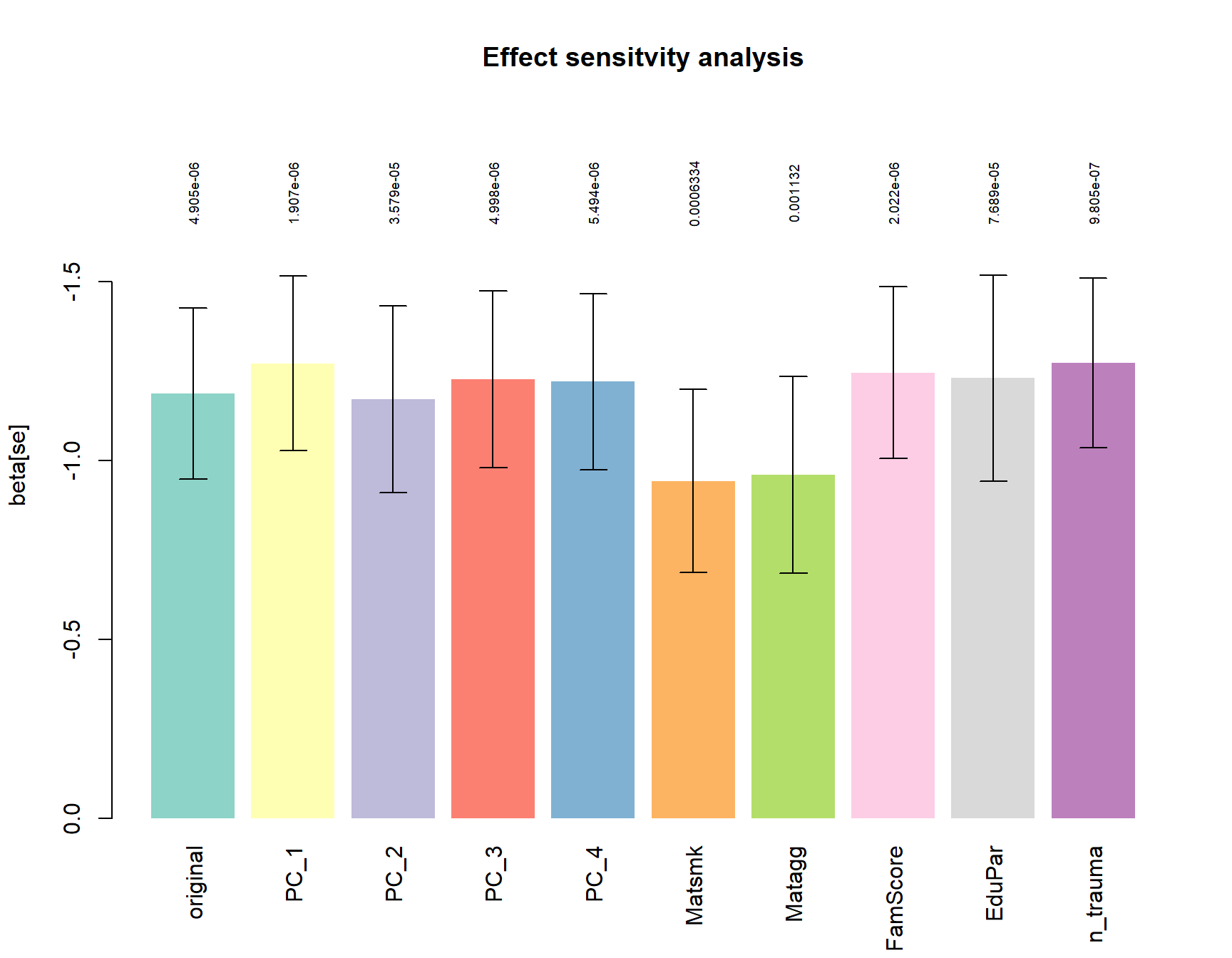
All models are corrected for:
site, Age, Pubstat, int_dis, medication, contraceptives, cigday_1,
site is included as random effect.
original: model defined as 0 + (1 | site) + Age + int_dis + medication + contraceptives + cigday_1 + V8 + group
all other models represent the original model + the variable of interest
Genomic location enrichment
Significant loci with a p-value <= 0.01 and a absolute log2 fold-change lager 0.5 were tested for enrichment in annotated genomic feature using fisher exact test.
Ranges=rowData(dds_filt)

TotTagsofInterest=sum(Ranges$WaldPvalue_groupCD<=thresholdp & abs(Ranges$groupCD)>thresholdLFC)

Resall=data.frame()
index = Ranges$WaldPvalue_groupCD<=thresholdp& abs(Ranges$groupCD)>thresholdLFC
for (feat in unique(Ranges$feature)){
  tmp=table(Ranges$feature == feat, signif=index)
  resfish=fisher.test(tmp)
  res = c(resfish$estimate, unlist(resfish$conf.int), resfish$p.value)
  Resall = rbind(Resall, res)
}
tmp=table(Ranges$tf_binding!="", signif=index)
resfish=fisher.test(tmp)
res = c(resfish$estimate, unlist(resfish$conf.int), resfish$p.value)
Resall = rbind(Resall, res)
tmp=table(Ranges$cpg=="cpg", signif=index)
resfish=fisher.test(tmp)
res = c(resfish$estimate, unlist(resfish$conf.int), resfish$p.value)
Resall = rbind(Resall, res)
colnames(Resall)=c("OR", "CI95L", "CI95U", "P")
rownames(Resall)=c(unique(Ranges$feature), "TF-binding", "CpG-island")
Resall$Beta = log(Resall$OR)
Resall$SE = (log(Resall$OR)-log(Resall$CI95L))/1.96
Resall$Padj=p.adjust(Resall$P, method = "bonferroni")

Resdown=data.frame()
index = Ranges$WaldPvalue_groupCD<=thresholdp & Ranges$groupCD<thresholdLFC
for (feat in unique(Ranges$feature)){
  tmp=table(Ranges$feature == feat, signif=index)
  resfish=fisher.test(tmp)
  res = c(resfish$estimate, unlist(resfish$conf.int), resfish$p.value)
  Resdown = rbind(Resdown, res)
}
tmp=table(Ranges$tf_binding!="", signif=index)
resfish=fisher.test(tmp)
res = c(resfish$estimate, unlist(resfish$conf.int), resfish$p.value)
Resdown = rbind(Resdown, res)
tmp=table(Ranges$cpg=="cpg", signif=index)
resfish=fisher.test(tmp)
res = c(resfish$estimate, unlist(resfish$conf.int), resfish$p.value)
Resdown = rbind(Resdown, res)
colnames(Resdown)=c("OR", "CI95L", "CI95U", "P")
rownames(Resdown)=c(unique(Ranges$feature), "TF-binding", "CpG-island")
Resdown$Beta = log(Resdown$OR)
Resdown$SE = (log(Resdown$OR)-log(Resdown$CI95L))/1.96
Resdown$Padj=p.adjust(Resdown$P, method = "bonferroni")

Resup=data.frame()
index = Ranges$WaldPvalue_groupCD<=thresholdp & Ranges$groupCD>thresholdLFC
for (feat in unique(Ranges$feature)){
  tmp=table(Ranges$feature == feat, signif=index)
  resfish=fisher.test(tmp)
  res = c(resfish$estimate, unlist(resfish$conf.int), resfish$p.value)
  Resup = rbind(Resup, res)
}
tmp=table(Ranges$tf_binding!="", signif=index)
resfish=fisher.test(tmp)
res = c(resfish$estimate, unlist(resfish$conf.int), resfish$p.value)
Resup = rbind(Resup, res)
tmp=table(Ranges$cpg=="cpg", signif=index)
resfish=fisher.test(tmp)
res = c(resfish$estimate, unlist(resfish$conf.int), resfish$p.value)
Resup = rbind(Resup, res)
colnames(Resup)=c("OR", "CI95L", "CI95U", "P")
rownames(Resup)=c(unique(Ranges$feature), "TF-binding", "CpG-island")
Resup$Beta = log(Resup$OR)
Resup$SE = (log(Resup$OR)-log(Resup$CI95L))/1.96
Resup$Padj=p.adjust(Resup$P, method = "bonferroni")

multiORplot(Resall, Pval = "P", Padj = "Padj", beta="Beta",SE = "SE", pheno="All diff. methylated loci")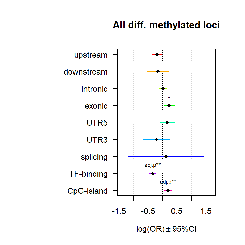
multiORplot(Resup, Pval = "P", Padj = "Padj", beta="Beta",SE = "SE", pheno="hypomethylated loci")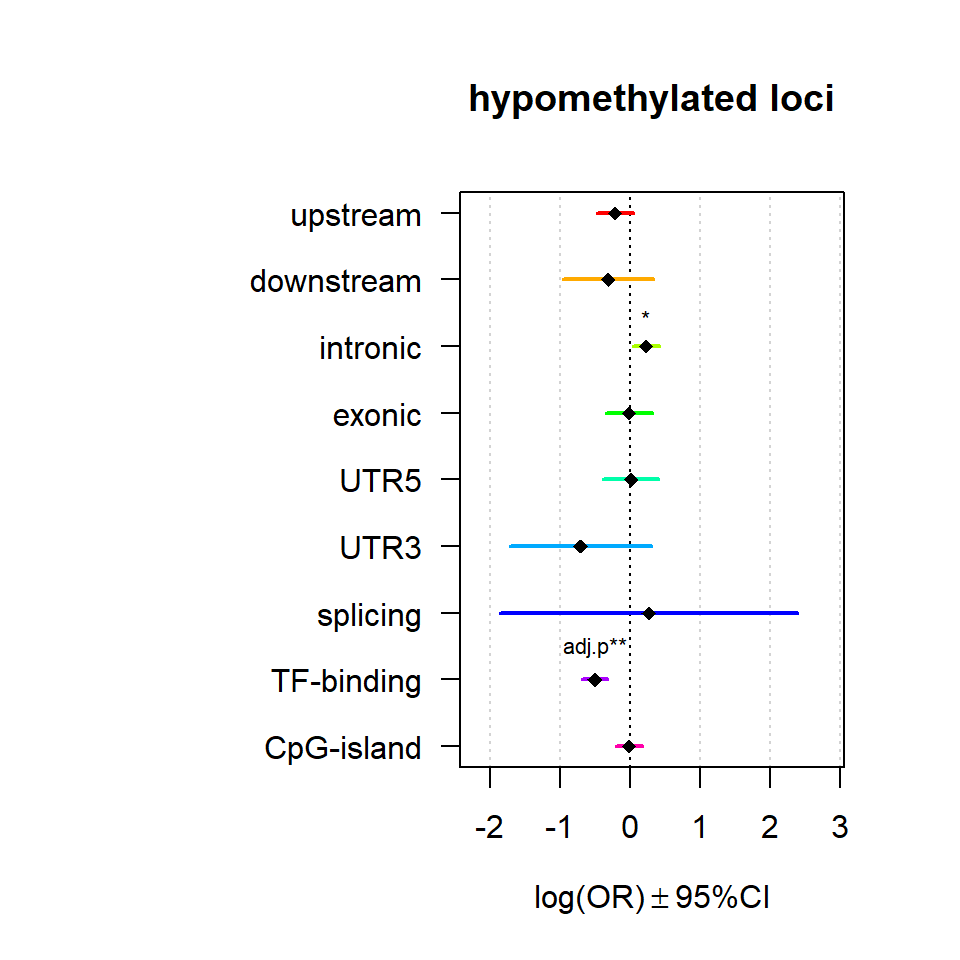
multiORplot(Resdown, Pval = "P", Padj = "Padj", beta="Beta",SE = "SE", pheno="Hypermethylated loci")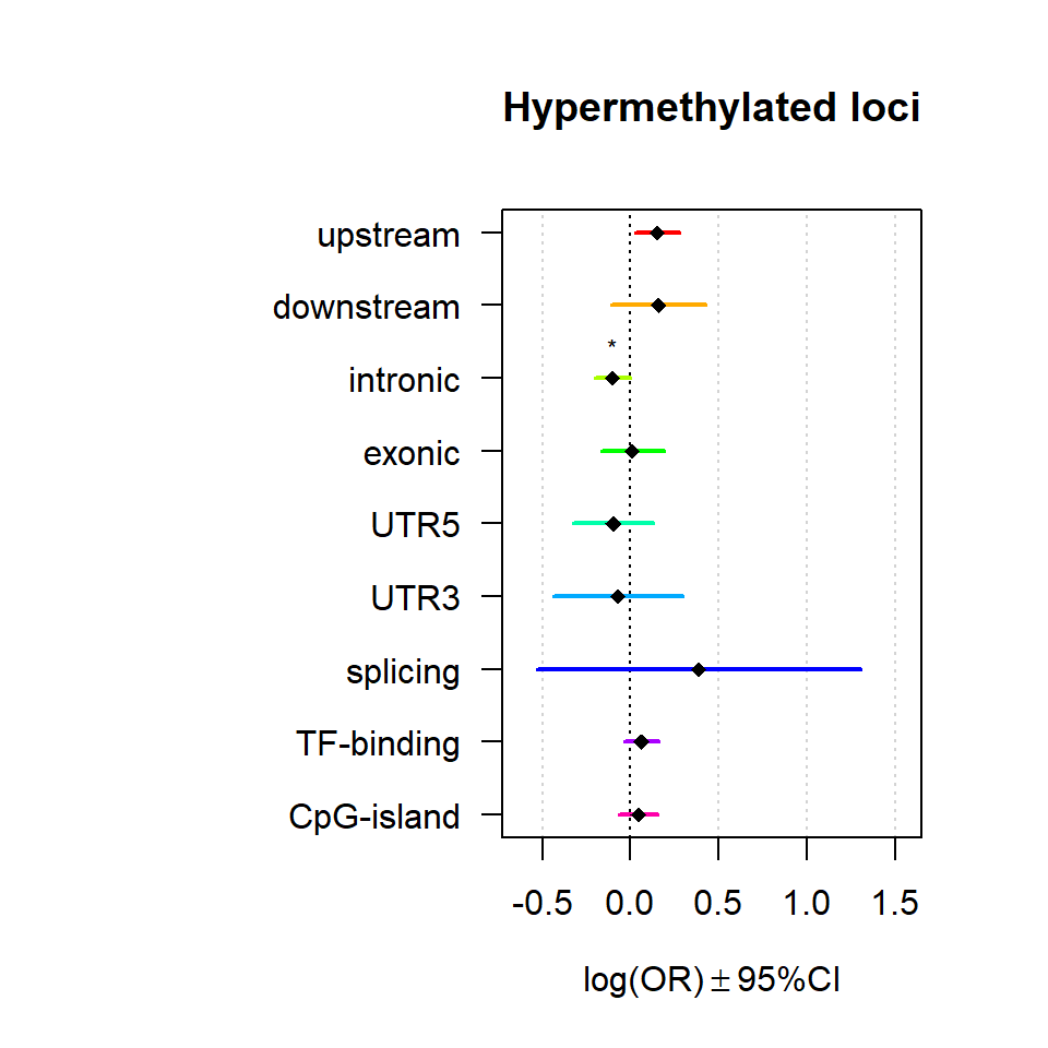
pdf(paste0(Home, "/output/functional_Enrichemnt.pdf"))
multiORplot(Resall, Pval = "P", Padj = "Padj", beta="Beta",SE = "SE", pheno="All diff. methylated loci")
multiORplot(Resup, Pval = "P", Padj = "Padj", beta="Beta",SE = "SE", pheno="hypomethylated loci")
multiORplot(Resdown, Pval = "P", Padj = "Padj", beta="Beta",SE = "SE", pheno="Hypermethylated loci")
dev.off()
png
2 GO-term Enrichment
Significant loci and differentially methylated regions with a p-value <= 0.01 and an absolute log2 fold-change lager 0.5 were tested for enrichment among GO-terms Molecular Function, Cellular Compartment and Biological Processes, KEGG pathways, Transcription factor Binding sites, Human Protein Atlas Tissue Expression, Human Phenotypes.
getGOresults = function(geneset, genereference){
  resgo = gost(geneset, organism = "hsapiens",
               correction_method = "g_SCS",
               domain_scope = "custom",
               sources = c("GO:BP", "GO:MF", "GO:CC"),
               custom_bg = genereference)
  if(length(resgo) != 0){
    return(resgo)
  } else {
    print("no significant results")
    return(NULL)
  }
}

gene_univers = getuniquegenes(as.data.frame(rowRanges(dds_filt))$gene)


idx = (results_Deseq$pvalue <= thresholdp &
         (abs(results_Deseq$log2FoldChange) > thresholdLFC))

genes_reg = getuniquegenes(as.data.frame(rowRanges(dds_filt))$gene[idx])


dmr_genes = unique(resultsdmr_table$name[resultsdmr_table$p.value<=thresholdp &
                   abs(resultsdmr_table$value)>=thresholdLFC])


Genes_of_interset = list("01_dmregions" = dmr_genes,
                         "02_dmtag" = genes_reg
                         )

gostres = getGOresults(Genes_of_interset, gene_univers)

gostplot(gostres, capped = TRUE, interactive = T)
p = gostplot(gostres, capped = TRUE, interactive = F)
toptab = gostres$result
pp = publish_gostplot(p, filename = paste0(Home,"/output/gostres.pdf"))The image is saved to C:/Users/chiocchetti/Projects/femNATCD_MethSeq/output/gostres.pdfwrite.xlsx2(toptab, file = paste0(Home,"/output/GOres.xlsx"), sheetName = "GO_enrichment")Kang Brain Module Enrichments
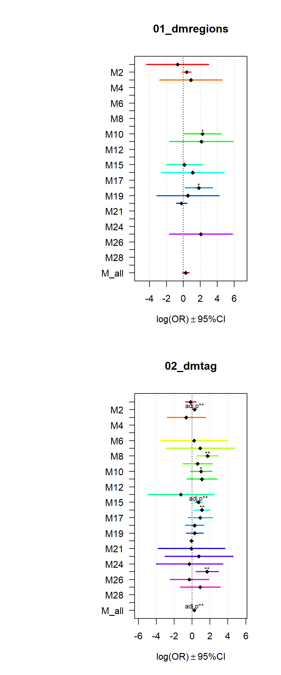
Gene sets identified to be deferentially methylated with a p-value <= 0.01 and an absolute log2 fold-change larger 0.5 were tested for enrichment among gene-modules coregulated during Brain expression.
# define Reference Universe

KangUnivers<- read.table(paste0(Home,"/data/KangUnivers.txt"), sep="\t", header=T)
colnames(KangUnivers)<-c("EntrezId","Symbol")

Kang_genes<-read.table(paste0(Home,"/data/Kang_dataset_genesMod_version2.txt"),sep="\t",header=TRUE)

#3)Generate Gene universe to be used for single gene lists
tmp=merge(KangUnivers,Kang_genes,by.y="EntrezGene",by.x="EntrezId",all=TRUE) #18826
KangUni_Final<-tmp[duplicated(tmp$EntrezId)==FALSE,] #18675


# Local analysis gene universe
Annotation_list<-data.frame(Symbol = gene_univers)

# match modules
Annotation_list$Module = Kang_genes$Module[match(Annotation_list$Symbol,Kang_genes$symbol)]

# check if overlapping in gene universes
Annotation_list$univers = Annotation_list$Symbol %in% KangUni_Final$Symbol

# drop duplicates
Annotation_list = Annotation_list[duplicated(Annotation_list$Symbol)==FALSE,]

# selct only genes that have been detected on both datasets
Annotation_list = Annotation_list[Annotation_list$univers==T,]

# final reference
UniversalGeneset=Annotation_list$Symbol

# define Gene lists to test
# sort and order Modules to be tested

Modules=unique(Annotation_list$Module)
Modules = Modules[! Modules %in% c(NA, "")]
Modules = Modules[order(as.numeric(gsub("M","",Modules)))]

GL_all=list()

for(i in Modules){
  GL_all[[i]]=Annotation_list$Symbol[Annotation_list$Module%in%i]
}
GL_all[["M_all"]]=Kang_genes$symbol[Kang_genes$Module %in% Modules]


GOI1 = Genes_of_interset

Resultsall=list()
for(j in names(GOI1)){
  Res = data.frame()
  for(i in names(GL_all)){
    Modulegene=GL_all[[i]]
    Factorgene=GOI1[[j]]
    Testframe<-fisher.test(table(factor(UniversalGeneset %in% Factorgene,levels=c("TRUE","FALSE")),
                                 factor(UniversalGeneset %in% Modulegene,levels=c("TRUE","FALSE"))))
    beta=log(Testframe$estimate)
    Res[i, "beta"] =beta
    Res[i, "SE"]=abs(beta-log(Testframe$conf.int[1]))/1.96
    Res[i, "Pval"]=Testframe$p.value
    Res[i, "OR"]=(Testframe$estimate)
    Res[i, "ORL"]=(Testframe$conf.int[1])
    Res[i, "ORU"]=(Testframe$conf.int[2])
  }
  Res$Padj = p.adjust(Res$Pval, method = "bonferroni")
  Resultsall[[j]] = Res

}
par(mfrow = c(2,1))
for (i in names(Resultsall)){
  multiORplot(datatoplot = Resultsall[[i]], pheno=i)
}
par(mfrow = c(1,1))
pdf(paste0(Home, "/output/BrainMod_Enrichemnt.pdf"))
for (i in names(Resultsall)){
  multiORplot(datatoplot = Resultsall[[i]], pheno=i)
}
dev.off()
png
2 Modsig = c()
for(r in names(Resultsall)){
a=rownames(Resultsall[[r]])[Resultsall[[r]]$Padj<=0.05]
Modsig = c(Modsig,a)
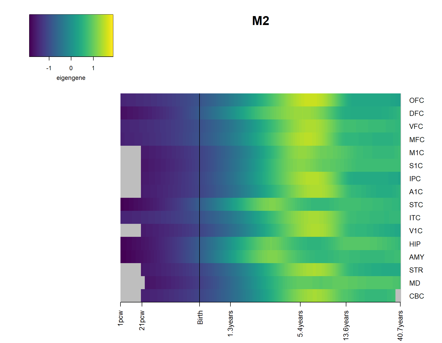
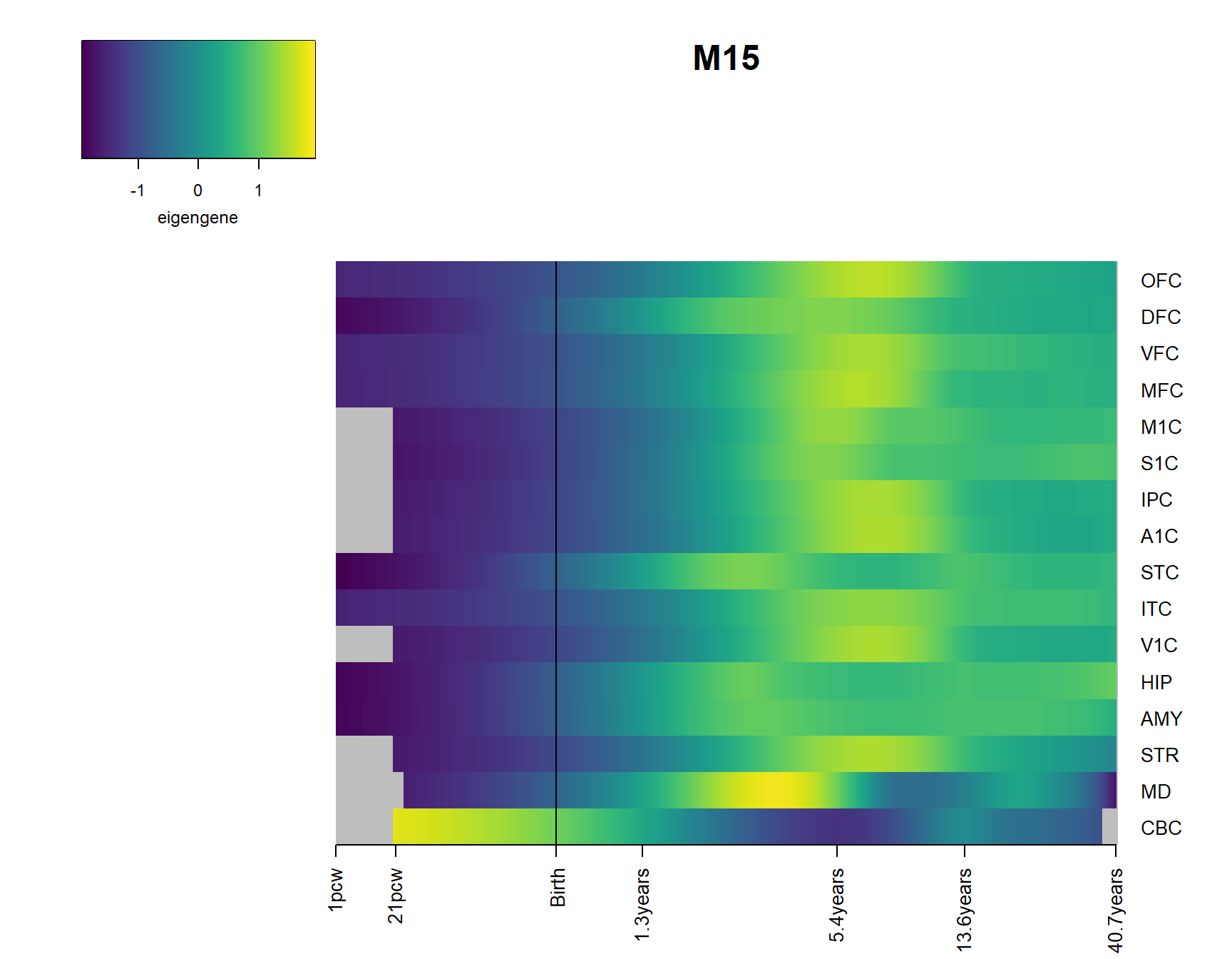
}# show brains and expression
Modsig2=unique(Modsig[Modsig!="M_all"])
load(paste0(Home,"/data/Kang_DataPreprocessing.RData")) #Load the Kang expression data of all genes
datExprPlot=matriz #Expression data of Kang loaded as Rdata object DataPreprocessing.RData
Genes = GL_all[names(GL_all)!="M_all"]
Genes_expression<-list()
pcatest<-list()
for (i in names(Genes)){
Genes_expression[[i]]<-matriz[,which(colnames(matriz) %in% Genes[[i]])]
pcatest[[i]]=prcomp(t(as.matrix(Genes_expression[[i]])),retx=TRUE)
}
# PCA test
PCA<-data.frame(pcatest[[1]]$rotation)
PCA$donor_name<-rownames(PCA)
PC1<-data.frame(PCA[,c(1,ncol(PCA))])
#Combining the age with expression data
list <- strsplit(sampleInfo$age, " ")
library("plyr")------------------------------------------------------------------------------You have loaded plyr after dplyr - this is likely to cause problems.
If you need functions from both plyr and dplyr, please load plyr first, then dplyr:
library(plyr); library(dplyr)------------------------------------------------------------------------------
Attache Paket: 'plyr'The following object is masked from 'package:matrixStats':
countThe following object is masked from 'package:IRanges':
descThe following object is masked from 'package:S4Vectors':
renameThe following objects are masked from 'package:dplyr':
arrange, count, desc, failwith, id, mutate, rename, summarise,
summarizeThe following object is masked from 'package:purrr':
compactdf <- ldply(list)
colnames(df) <- c("Age", "time")
sampleInfo<-cbind(sampleInfo[,1:9],df)
sampleInfo$Age<-as.numeric(sampleInfo$Age)
sampleInfo$period<-ifelse(sampleInfo$time=="pcw",sampleInfo$Age*7,ifelse(sampleInfo$time=="yrs",sampleInfo$Age*365+270,ifelse(sampleInfo$time=="mos",sampleInfo$Age*30+270,NA)))
#We need it just for the donor names
PCA_matrix<-merge.with.order(PC1,sampleInfo,by.y="SampleID",by.x="donor_name",keep_order=1)
#Select which have phenotype info present
matriz2<-matriz[which(rownames(matriz) %in% PCA_matrix$donor_name),]
FactorGenes_expression<-list()
#Factors here mean modules
for (i in names(Genes)){
FactorGenes_expression[[i]]<-matriz2[,which(colnames(matriz2) %in% Genes[[i]])]
}
FactorseGE<-list()
for (i in names(Genes)){
FactorseGE[[i]]<-FactorGenes_expression[[i]]
}
allModgenes=NULL
colors=vector()
for ( i in names(Genes)){
allModgenes=cbind(allModgenes,FactorseGE[[i]])
colors=c(colors, rep(i, ncol(FactorseGE[[i]])))
}
lengths=unlist(lapply(FactorGenes_expression, ncol), use.names = F)
MEorig=moduleEigengenes(allModgenes, colors)
PCA_matrixfreeze=PCA_matrix
index=!PCA_matrix$structure_acronym %in% c("URL", "DTH", "CGE","LGE", "MGE", "Ocx", "PCx", "M1C-S1C","DIE", "TCx", "CB")
PCA_matrix=PCA_matrix[index,]
ME = MEorig$eigengenes[index,]
matsel = matriz2[index,]
colnames(ME) = gsub("ME", "", colnames(ME))
timepoints=seq(56,15000, length.out=1000)
matrix(c("CB", "THA", "CBC", "MD"), ncol=2 ) -> cnm
brainheatmap=function(Module){
MEmod=ME[,Module]
toplot=data.frame(matrix(NA, nrow=length(table(PCA_matrix$structure_acronym)), ncol=998))
rownames(toplot)=unique(PCA_matrix$structure_acronym)
target <- c("OFC", "DFC", "VFC", "MFC","M1C","S1C","IPC","A1C","STC","ITC","V1C","HIP","AMY","STR","MD","CBC")
toplot<-toplot[c(6,2,8,5,11,12,10,9,7,4,14,3,1,13,16,15),]
for ( i in unique(PCA_matrix$structure_acronym)){
index=PCA_matrix$structure_acronym==i
LOESS=loess(MEmod[index]~PCA_matrix$period[index])
toplot[i,]=predict(LOESS,newdata = round(exp(seq(log(56),log(15000), length.out=998)),2))
colnames(toplot)[c(1,77,282,392,640,803,996)]<-
c("1pcw","21pcw","Birth","1.3years","5.4years","13.6years","40.7years")
}
cols=viridis(100)
labvec <- c(rep(NA, 1000))
labvec[c(1,77,282,392,640,803,996)] <- c("1pcw","21pcw","Birth","1.3years","5.4years","13.6years","40.7years")
toplot<-toplot[,1:998]
date<-c(1:998)
dateY<-paste0(round(date/365,2),"_Years")
names(toplot)<-dateY
par(xpd=FALSE)
heatmap.2(as.matrix(toplot), col = cols,
main=Module,
trace = "none",
na.color = "grey",
Colv = F, Rowv = F,
labCol = labvec,
#breaks = seq(-0.1,0.1, length.out=101),
symkey = T,
scale = "row",
key.title = "",
dendrogram = "none",
key.xlab = "eigengene",
density.info = "none",
#main=paste("Module",1),
srtCol=90,
tracecol = "none",
cexRow = 1,
add.expr=eval.parent(abline(v=282),
axis(1,at=c(1,77,282,392,640,803,996),
labels =FALSE)),cexCol = 1)
}
brainheatmap_gene=function(Genename){
MEmod=matsel[,Genename]
toplot=data.frame(matrix(NA, nrow=length(table(PCA_matrix$structure_acronym)), ncol=998))
rownames(toplot)=unique(PCA_matrix$structure_acronym)
target <- c("OFC", "DFC", "VFC", "MFC","M1C","S1C","IPC","A1C","STC","ITC","V1C","HIP","AMY","STR","MD","CBC")
toplot<-toplot[c(6,2,8,5,11,12,10,9,7,4,14,3,1,13,16,15),]
for ( i in unique(PCA_matrix$structure_acronym)){
index=PCA_matrix$structure_acronym==i
LOESS=loess(MEmod[index]~PCA_matrix$period[index])
toplot[i,]=predict(LOESS,newdata = round(exp(seq(log(56),log(15000), length.out=998)),2))
colnames(toplot)[c(1,77,282,392,640,803,996)]<-
c("1pcw","21pcw","Birth","1.3years","5.4years","13.6years","40.7years")
}
cols=viridis(100)
labvec <- c(rep(NA, 1000))
labvec[c(1,77,282,392,640,803,996)] <- c("1pcw","21pcw","Birth","1.3years","5.4years","13.6years","40.7years")
toplot<-toplot[,1:998]
date<-c(1:998)
dateY<-paste0(round(date/365,2),"_Years")
names(toplot)<-dateY
par(xpd=FALSE)
heatmap.2(as.matrix(toplot), col = cols,
main=Genename,
trace = "none",
na.color = "grey",
Colv = F, Rowv = F,
labCol = labvec,
#breaks = seq(-0.1,0.1, length.out=101),
symkey = F,
scale = "none",
key.title = "",
dendrogram = "none",
key.xlab = "eigengene",
density.info = "none",
#main=paste("Module",1),
#srtCol=90,
tracecol = "none",
cexRow = 1,
add.expr=eval.parent(abline(v=282),
axis(1,at=c(1,77,282,392,640,803,996),
labels =FALSE))
,cexCol = 1)
}
brainheatmap_gene("SLITRK5")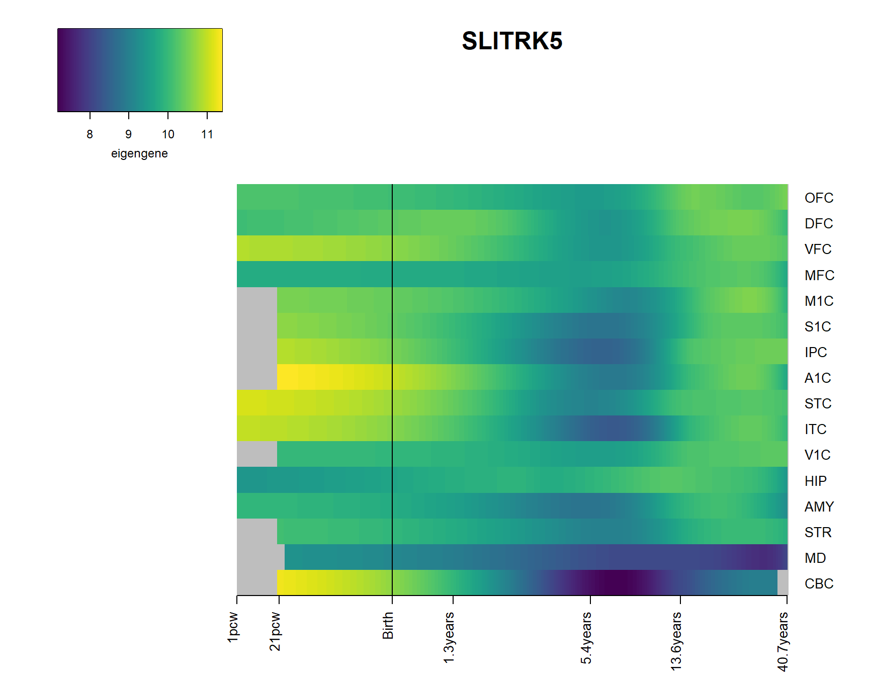
for(Module in Modsig2){
  brainheatmap(Module)
}
pdf(paste0(Home, "/output/Brain_Module_Heatmap.pdf"))

brainheatmap_gene("SLITRK5")
for(Module in Modsig2){
  brainheatmap(Module)
}
dev.off()
png
2 SEM
dropfact=c("site", "0", "group")

modelFact=strsplit(as.character(design(dds_filt))[2], " \\+ ")[[1]]


Patdata=as.data.frame(colData(dds_filt))

load(paste0(Home, "/output/envFact.RData"))

envFact=envFact[!envFact %in% dropfact]
modelFact=modelFact[!modelFact %in% dropfact]

EpiMarker = c()

# TopHit
Patdata$Epi_TopHit=log2_cpm[base::which.min(results_Deseq$pvalue),]

# 1PC of all diff met
tmp=glmpca(log2_cpm[base::which(results_Deseq$pvalue<=thresholdp),], 1)

Patdata$Epi_all= tmp$factors$dim1

EpiMarker = c(EpiMarker, "Epi_TopHit", "Epi_all")

#Brain Modules

Epitestset=GL_all[Modsig]

for(n in names(Epitestset)){
  index=gettaglistforgenelist(genelist = Epitestset[[n]], dds_filt)
  index = base::intersect(index, base::which(results_Deseq$pvalue<=thresholdp))
  # get eigenvalue
  epiname=paste0("Epi_",n)
  tmp=glmpca(log2_cpm[index,], 1)
  Patdata[,epiname]= tmp$factors$dim1
  EpiMarker = c(EpiMarker, epiname)
}

cormat = cor(apply(Patdata[,c("group", envFact, modelFact, EpiMarker)] %>% mutate_all(as.numeric), 2, minmax_scaling),
             use = "pairwise.complete.obs")

par(mfrow=c(1,2))
corrplot(cormat, main="correlations")
corrplot(cormat, order = "hclust", main="scaled correlations")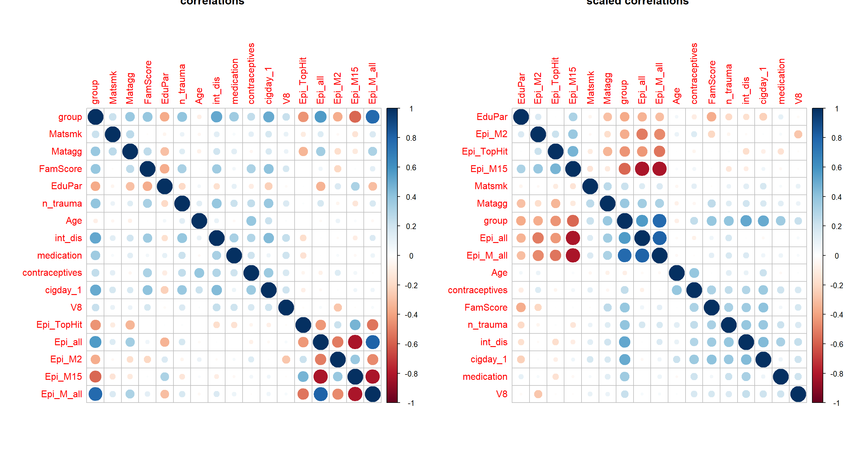
fullmodEnv=paste(unique(envFact,modelFact), sep = "+", collapse = "+")

Dataset = Patdata[,c("group", envFact,modelFact,EpiMarker)]

model = "
Epi~1+a*Matsmk+b*Matagg+c*FamScore+d*EduPar+e*n_trauma+Age+int_dis+medication+contraceptives+cigday_1+V8
group~1+f*Matsmk+g*Matagg+h*FamScore+i*EduPar+j*n_trauma+Age+int_dis+medication+contraceptives+cigday_1+z*Epi

#direct
directMatsmk := f
directMatagg := g
directFamScore := h
directEduPar := i
directn_trauma := j

#indirect
EpiMatsmk := a*z
EpiMatagg := b*z
EpiFamScore := c*z
EpiEduPar := d*z
Epin_trauma := e*z

total := f + g + h + i + j + (a*z)+(b*z)+(c*z)+(d*z)+(e*z)

Epi~~Epi
group~~group
"

Netlist = list()

for (marker in EpiMarker) {
  Dataset$Epi = Dataset[,marker]
  Datasetscaled = Dataset %>% mutate_if(is.numeric, minmax_scaling)
  Datasetscaled = Datasetscaled %>% mutate_if(is.factor, ~ as.numeric(.)-1)

  fit<-lavaan(model,data=Datasetscaled)

  sink(paste0(Home,"/output/SEM_summary_group",marker,".txt"))
  summary(fit)
  print(fitMeasures(fit))
  print(parameterEstimates(fit))
  sink()
  print("############################")
  print("############################")
  print(marker)
  print("############################")
  print("############################")
  summary(fit)
  fitMeasures(fit)
  parameterEstimates(fit)


  #SOURCE FOR PLOT https://stackoverflow.com/questions/51270032/how-can-i-display-only-significant-path-lines-on-a-path-diagram-r-lavaan-sem
  restab=lavaan::standardizedSolution(fit) %>% dplyr::filter(!is.na(pvalue)) %>%
    arrange(desc(pvalue)) %>% mutate_if("is.numeric","round",3) %>%
    dplyr::select(-ci.lower,-ci.upper,-z)

  pvalue_cutoff <- 0.05

  obj <- semPlot:::semPlotModel(fit)
  original_Pars <- obj@Pars
  check_Pars <- obj@Pars %>% dplyr:::filter(!(edge %in% c("int","<->") | lhs == rhs)) # this is the list of parameter to sift thru
  keep_Pars <- obj@Pars %>% dplyr:::filter(edge %in% c("int","<->") | lhs == rhs) # this is the list of parameter to keep asis

  test_against <- lavaan::standardizedSolution(fit) %>% dplyr::filter(pvalue < pvalue_cutoff, rhs != lhs)

  # for some reason, the rhs and lhs are reversed in the standardizedSolution() output, for some of the values
  # I'll have to reverse it myself, and test against both orders

  test_against_rev <- test_against %>% dplyr::rename(rhs2 = lhs, lhs = rhs) %>% dplyr::rename(rhs = rhs2)

  checked_Pars <-
    check_Pars %>% semi_join(test_against, by = c("lhs", "rhs")) %>% bind_rows(
      check_Pars %>% semi_join(test_against_rev, by = c("lhs", "rhs"))
    )

  obj@Pars <- keep_Pars %>% bind_rows(checked_Pars) %>%
    mutate_if("is.numeric","round",3) %>%
    mutate_at(c("lhs","rhs"),~gsub("Epi", marker,.))

  obj@Vars = obj@Vars %>% mutate_at(c("name"),~gsub("Epi", marker,.))

  DF = obj@Pars
  DF = DF[DF$lhs!=DF$rhs,]
  DF = DF[abs(DF$std)>0.1,]

  DF = DF[DF$edge == "~>",] # only include directly modelled effects in figure

  nodes <- data.frame(id=obj@Vars$name, label = obj@Vars$name)
  nodes$color<-Dark8[8]
  nodes$color[nodes$label == "group"] = Dark8[3]
  nodes$color[nodes$label == marker] = Dark8[4]
  nodes$color[nodes$label %in% envFact] = Dark8[5]

  edges <- data.frame(from = DF$lhs,
                      to = DF$rhs,
                      width=abs(DF$std),
                      arrows ="to")

  edges$dashes = F
  edges$label =  DF$std
  edges$color=c("firebrick", "forestgreen")[1:2][factor(sign(DF$std), levels=c(-1,0,1),labels=c(1,2,2))]
  edges$width=2
  cexlab = 18
  plotnet<- visNetwork(nodes, edges,
                       main=list(text=marker,
                                 style="font-family:arial;font-size:20px;text-align:center"),
                       submain=list(text="significant paths",
                                    style="font-family:arial;text-align:center")) %>%
    visEdges(arrows =list(to = list(enabled = TRUE, scaleFactor = 0.7)),
                       font=list(size=cexlab, style="font-family:arial;text-align:center")) %>%
    visNodes(font=list(size=cexlab, style="font-family:arial;text-align:center")) %>%

    visPhysics(enabled = T, solver = "forceAtlas2Based")


  Netlist[[marker]] = plotnet
  htmlfile = paste0(Home,"/output/SEMplot_",marker,".html")
  visSave(plotnet, htmlfile)
  webshot(paste0(Home,"/output/SEMplot_",marker,".html"), zoom = 1,
          file = paste0(Home,"/output/SEMplot_",marker,".png"))

}
[1] "############################"
[1] "############################"
[1] "Epi_TopHit"
[1] "############################"
[1] "############################"
lavaan 0.6-7 ended normally after 40 iterations
Estimator ML
Optimization method NLMINB
Number of free parameters 26
Used Total
Number of observations 80 99
Model Test User Model:
Test statistic 0.460
Degrees of freedom 1
P-value (Chi-square) 0.498
Parameter Estimates:
Standard errors Standard
Information Expected
Information saturated (h1) model Structured
Regressions:
Estimate Std.Err z-value P(>|z|)
Epi ~
Matsmk (a) -0.033 0.045 -0.731 0.465
Matagg (b) -0.014 0.068 -0.213 0.831
FamScore (c) 0.056 0.064 0.887 0.375
EduPar (d) -0.038 0.082 -0.468 0.640
n_trauma (e) 0.085 0.088 0.964 0.335
Age -0.090 0.087 -1.036 0.300
int_dis -0.074 0.047 -1.580 0.114
medication -0.044 0.051 -0.876 0.381
contrcptvs -0.017 0.046 -0.361 0.718
cigday_1 -0.111 0.090 -1.228 0.219
V8 -0.089 0.262 -0.339 0.735
group ~
Matsmk (f) 0.001 0.080 0.008 0.994
Matagg (g) 0.197 0.122 1.611 0.107
FamScore (h) 0.018 0.115 0.160 0.873
EduPar (i) -0.470 0.148 -3.184 0.001
n_trauma (j) 0.277 0.158 1.752 0.080
Age -0.360 0.156 -2.310 0.021
int_dis 0.179 0.085 2.111 0.035
medication 0.277 0.092 3.021 0.003
contrcptvs -0.019 0.083 -0.227 0.820
cigday_1 0.667 0.164 4.077 0.000
Epi (z) -1.010 0.201 -5.030 0.000
Intercepts:
Estimate Std.Err z-value P(>|z|)
.Epi 0.843 0.159 5.320 0.000
.group 1.342 0.206 6.519 0.000
Variances:
Estimate Std.Err z-value P(>|z|)
.Epi 0.023 0.004 6.325 0.000
.group 0.075 0.012 6.325 0.000
Defined Parameters:
Estimate Std.Err z-value P(>|z|)
directMatsmk 0.001 0.080 0.008 0.994
directMatagg 0.197 0.122 1.611 0.107
directFamScore 0.018 0.115 0.160 0.873
directEduPar -0.470 0.148 -3.184 0.001
directn_trauma 0.277 0.158 1.752 0.080
EpiMatsmk 0.033 0.045 0.723 0.470
EpiMatagg 0.015 0.069 0.213 0.831
EpiFamScore -0.057 0.065 -0.874 0.382
EpiEduPar 0.039 0.083 0.466 0.641
Epin_trauma -0.086 0.090 -0.947 0.344
total -0.034 0.319 -0.107 0.915
[1] "############################"
[1] "############################"
[1] "Epi_all"
[1] "############################"
[1] "############################"
lavaan 0.6-7 ended normally after 47 iterations
Estimator ML
Optimization method NLMINB
Number of free parameters 26
Used Total
Number of observations 80 99
Model Test User Model:
Test statistic 0.604
Degrees of freedom 1
P-value (Chi-square) 0.437
Parameter Estimates:
Standard errors Standard
Information Expected
Information saturated (h1) model Structured
Regressions:
Estimate Std.Err z-value P(>|z|)
Epi ~
Matsmk (a) 0.014 0.023 0.614 0.539
Matagg (b) 0.023 0.036 0.635 0.525
FamScore (c) -0.037 0.033 -1.093 0.274
EduPar (d) -0.090 0.043 -2.096 0.036
n_trauma (e) 0.025 0.046 0.542 0.588
Age 0.034 0.046 0.747 0.455
int_dis 0.023 0.025 0.923 0.356
medication 0.007 0.027 0.276 0.783
contrcptvs -0.016 0.024 -0.646 0.518
cigday_1 0.022 0.047 0.463 0.643
V8 0.060 0.138 0.437 0.662
group ~
Matsmk (f) -0.017 0.044 -0.386 0.700
Matagg (g) 0.134 0.068 1.980 0.048
FamScore (h) 0.088 0.063 1.381 0.167
EduPar (i) -0.122 0.084 -1.460 0.144
n_trauma (j) 0.110 0.087 1.264 0.206
Age -0.381 0.086 -4.446 0.000
int_dis 0.172 0.046 3.714 0.000
medication 0.296 0.050 5.880 0.000
contrcptvs 0.051 0.046 1.102 0.270
cigday_1 0.701 0.090 7.828 0.000
Epi (z) 3.432 0.211 16.292 0.000
Intercepts:
Estimate Std.Err z-value P(>|z|)
.Epi 0.134 0.083 1.608 0.108
.group -0.033 0.080 -0.412 0.681
Variances:
Estimate Std.Err z-value P(>|z|)
.Epi 0.006 0.001 6.325 0.000
.group 0.023 0.004 6.325 0.000
Defined Parameters:
Estimate Std.Err z-value P(>|z|)
directMatsmk -0.017 0.044 -0.386 0.700
directMatagg 0.134 0.068 1.980 0.048
directFamScore 0.088 0.063 1.381 0.167
directEduPar -0.122 0.084 -1.460 0.144
directn_trauma 0.110 0.087 1.264 0.206
EpiMatsmk 0.049 0.080 0.614 0.540
EpiMatagg 0.078 0.123 0.635 0.526
EpiFamScore -0.125 0.115 -1.091 0.275
EpiEduPar -0.311 0.149 -2.079 0.038
Epin_trauma 0.086 0.159 0.542 0.588
total -0.031 0.319 -0.096 0.923
[1] "############################"
[1] "############################"
[1] "Epi_M2"
[1] "############################"
[1] "############################"
lavaan 0.6-7 ended normally after 41 iterations
Estimator ML
Optimization method NLMINB
Number of free parameters 26
Used Total
Number of observations 80 99
Model Test User Model:
Test statistic 0.173
Degrees of freedom 1
P-value (Chi-square) 0.678
Parameter Estimates:
Standard errors Standard
Information Expected
Information saturated (h1) model Structured
Regressions:
Estimate Std.Err z-value P(>|z|)
Epi ~
Matsmk (a) 0.009 0.033 0.272 0.786
Matagg (b) -0.017 0.051 -0.328 0.743
FamScore (c) -0.054 0.047 -1.133 0.257
EduPar (d) -0.010 0.061 -0.164 0.870
n_trauma (e) 0.018 0.066 0.277 0.782
Age -0.042 0.065 -0.646 0.518
int_dis -0.010 0.035 -0.274 0.784
medication 0.018 0.038 0.473 0.636
contrcptvs 0.074 0.035 2.145 0.032
cigday_1 -0.058 0.067 -0.866 0.386
V8 -0.522 0.195 -2.674 0.007
group ~
Matsmk (f) 0.039 0.083 0.469 0.639
Matagg (g) 0.194 0.126 1.535 0.125
FamScore (h) -0.097 0.119 -0.815 0.415
EduPar (i) -0.448 0.152 -2.943 0.003
n_trauma (j) 0.233 0.162 1.434 0.152
Age -0.295 0.160 -1.844 0.065
int_dis 0.227 0.086 2.629 0.009
medication 0.341 0.094 3.619 0.000
contrcptvs 0.078 0.088 0.883 0.377
cigday_1 0.702 0.168 4.172 0.000
Epi (z) -1.153 0.267 -4.319 0.000
Intercepts:
Estimate Std.Err z-value P(>|z|)
.Epi 0.886 0.118 7.504 0.000
.group 1.236 0.210 5.887 0.000
Variances:
Estimate Std.Err z-value P(>|z|)
.Epi 0.013 0.002 6.325 0.000
.group 0.080 0.013 6.325 0.000
Defined Parameters:
Estimate Std.Err z-value P(>|z|)
directMatsmk 0.039 0.083 0.469 0.639
directMatagg 0.194 0.126 1.535 0.125
directFamScore -0.097 0.119 -0.815 0.415
directEduPar -0.448 0.152 -2.943 0.003
directn_trauma 0.233 0.162 1.434 0.152
EpiMatsmk -0.010 0.038 -0.271 0.786
EpiMatagg 0.019 0.058 0.327 0.744
EpiFamScore 0.062 0.056 1.096 0.273
EpiEduPar 0.012 0.071 0.164 0.870
Epin_trauma -0.021 0.076 -0.277 0.782
total -0.019 0.316 -0.059 0.953
[1] "############################"
[1] "############################"
[1] "Epi_M15"
[1] "############################"
[1] "############################"
lavaan 0.6-7 ended normally after 40 iterations
Estimator ML
Optimization method NLMINB
Number of free parameters 26
Used Total
Number of observations 80 99
Model Test User Model:
Test statistic 1.526
Degrees of freedom 1
P-value (Chi-square) 0.217
Parameter Estimates:
Standard errors Standard
Information Expected
Information saturated (h1) model Structured
Regressions:
Estimate Std.Err z-value P(>|z|)
Epi ~
Matsmk (a) -0.055 0.046 -1.192 0.233
Matagg (b) 0.074 0.071 1.046 0.296
FamScore (c) 0.113 0.066 1.706 0.088
EduPar (d) 0.229 0.085 2.683 0.007
n_trauma (e) -0.062 0.092 -0.680 0.497
Age -0.088 0.090 -0.973 0.331
int_dis -0.065 0.049 -1.325 0.185
medication -0.024 0.053 -0.456 0.649
contrcptvs 0.032 0.048 0.660 0.509
cigday_1 -0.052 0.094 -0.552 0.581
V8 0.007 0.273 0.026 0.979
group ~
Matsmk (f) -0.050 0.058 -0.862 0.389
Matagg (g) 0.324 0.089 3.647 0.000
FamScore (h) 0.134 0.084 1.592 0.111
EduPar (i) -0.078 0.112 -0.700 0.484
n_trauma (j) 0.091 0.114 0.801 0.423
Age -0.409 0.113 -3.620 0.000
int_dis 0.158 0.061 2.579 0.010
medication 0.285 0.066 4.308 0.000
contrcptvs 0.048 0.060 0.797 0.426
cigday_1 0.701 0.118 5.963 0.000
Epi (z) -1.537 0.140 -10.984 0.000
Intercepts:
Estimate Std.Err z-value P(>|z|)
.Epi 0.597 0.165 3.619 0.000
.group 1.462 0.126 11.586 0.000
Variances:
Estimate Std.Err z-value P(>|z|)
.Epi 0.025 0.004 6.325 0.000
.group 0.040 0.006 6.325 0.000
Defined Parameters:
Estimate Std.Err z-value P(>|z|)
directMatsmk -0.050 0.058 -0.862 0.389
directMatagg 0.324 0.089 3.647 0.000
directFamScore 0.134 0.084 1.592 0.111
directEduPar -0.078 0.112 -0.700 0.484
directn_trauma 0.091 0.114 0.801 0.423
EpiMatsmk 0.085 0.072 1.185 0.236
EpiMatagg -0.114 0.109 -1.041 0.298
EpiFamScore -0.173 0.103 -1.686 0.092
EpiEduPar -0.352 0.135 -2.606 0.009
Epin_trauma 0.096 0.141 0.678 0.498
total -0.037 0.319 -0.117 0.907
[1] "############################"
[1] "############################"
[1] "Epi_M_all"
[1] "############################"
[1] "############################"
lavaan 0.6-7 ended normally after 59 iterations
Estimator ML
Optimization method NLMINB
Number of free parameters 26
Used Total
Number of observations 80 99
Model Test User Model:
Test statistic 0.191
Degrees of freedom 1
P-value (Chi-square) 0.662
Parameter Estimates:
Standard errors Standard
Information Expected
Information saturated (h1) model Structured
Regressions:
Estimate Std.Err z-value P(>|z|)
Epi ~
Matsmk (a) 0.025 0.075 0.330 0.742
Matagg (b) 0.132 0.114 1.162 0.245
FamScore (c) -0.102 0.106 -0.956 0.339
EduPar (d) -0.281 0.137 -2.043 0.041
n_trauma (e) 0.074 0.147 0.506 0.613
Age 0.122 0.146 0.836 0.403
int_dis 0.085 0.079 1.082 0.279
medication 0.050 0.085 0.589 0.556
contrcptvs -0.074 0.078 -0.948 0.343
cigday_1 0.168 0.151 1.114 0.265
V8 0.285 0.439 0.649 0.516
group ~
Matsmk (f) 0.003 0.031 0.085 0.932
Matagg (g) 0.059 0.047 1.246 0.213
FamScore (h) 0.081 0.044 1.827 0.068
EduPar (i) -0.109 0.058 -1.871 0.061
n_trauma (j) 0.115 0.061 1.894 0.058
Age -0.400 0.060 -6.669 0.000
int_dis 0.148 0.032 4.567 0.000
medication 0.263 0.035 7.478 0.000
contrcptvs 0.080 0.032 2.494 0.013
cigday_1 0.580 0.063 9.210 0.000
Epi (z) 1.157 0.046 25.082 0.000
Intercepts:
Estimate Std.Err z-value P(>|z|)
.Epi 0.288 0.265 1.085 0.278
.group 0.028 0.054 0.520 0.603
Variances:
Estimate Std.Err z-value P(>|z|)
.Epi 0.065 0.010 6.325 0.000
.group 0.011 0.002 6.325 0.000
Defined Parameters:
Estimate Std.Err z-value P(>|z|)
directMatsmk 0.003 0.031 0.085 0.932
directMatagg 0.059 0.047 1.246 0.213
directFamScore 0.081 0.044 1.827 0.068
directEduPar -0.109 0.058 -1.871 0.061
directn_trauma 0.115 0.061 1.894 0.058
EpiMatsmk 0.028 0.086 0.330 0.742
EpiMatagg 0.153 0.132 1.161 0.246
EpiFamScore -0.118 0.123 -0.955 0.340
EpiEduPar -0.325 0.160 -2.037 0.042
Epin_trauma 0.086 0.170 0.506 0.613
total -0.027 0.318 -0.085 0.932rmd_paths <-paste0(tempfile(c(names(Netlist))),".Rmd")
names(rmd_paths) <- names(Netlist)
for (n in names(rmd_paths)) {
sink(file = rmd_paths[n])
cat(" \n",
"```{r, echo = FALSE}",
"Netlist[[n]]",
"```",
sep = " \n")
sink()
}Interactive results SEM analysis
only direct effects with a significant standardized effect of p<0.05 are shown.
    for (n in names(rmd_paths)) {
        cat(knitr::knit_child(rmd_paths[[n]],
                              quiet= TRUE))
        file.remove(rmd_paths[[n]])
    }
sessionInfo()R version 4.0.3 (2020-10-10)
Platform: x86_64-w64-mingw32/x64 (64-bit)
Running under: Windows 10 x64 (build 19042)
Matrix products: default
Random number generation:
RNG: Mersenne-Twister
Normal: Inversion
Sample: Rounding
locale:
[1] LC_COLLATE=German_Germany.1252 LC_CTYPE=German_Germany.1252
[3] LC_MONETARY=German_Germany.1252 LC_NUMERIC=C
[5] LC_TIME=German_Germany.1252
attached base packages:
[1] parallel stats4 stats graphics grDevices utils datasets
[8] methods base
other attached packages:
[1] plyr_1.8.6 scales_1.1.1
[3] RCircos_1.2.1 compareGroups_4.4.6
[5] lme4_1.1-26 Matrix_1.2-18
[7] webshot_0.5.2 visNetwork_2.0.9
[9] org.Hs.eg.db_3.12.0 AnnotationDbi_1.52.0
[11] xlsx_0.6.5 gprofiler2_0.2.0
[13] BiocParallel_1.24.1 kableExtra_1.3.1
[15] glmpca_0.2.0 knitr_1.30
[17] DESeq2_1.30.0 SummarizedExperiment_1.20.0
[19] Biobase_2.50.0 MatrixGenerics_1.2.0
[21] matrixStats_0.57.0 GenomicRanges_1.42.0
[23] GenomeInfoDb_1.26.2 IRanges_2.24.1
[25] S4Vectors_0.28.1 BiocGenerics_0.36.0
[27] forcats_0.5.0 stringr_1.4.0
[29] dplyr_1.0.2 purrr_0.3.4
[31] readr_1.4.0 tidyr_1.1.2
[33] tibble_3.0.4 tidyverse_1.3.0
[35] semPlot_1.1.2 lavaan_0.6-7
[37] viridis_0.5.1 viridisLite_0.3.0
[39] WGCNA_1.69 fastcluster_1.1.25
[41] dynamicTreeCut_1.63-1 ggplot2_3.3.3
[43] gplots_3.1.1 corrplot_0.84
[45] RColorBrewer_1.1-2 workflowr_1.6.2
loaded via a namespace (and not attached):
[1] coda_0.19-4 bit64_4.0.5 DelayedArray_0.16.0
[4] data.table_1.13.6 rpart_4.1-15 RCurl_1.98-1.2
[7] doParallel_1.0.16 generics_0.1.0 preprocessCore_1.52.1
[10] callr_3.5.1 RSQLite_2.2.2 mice_3.12.0
[13] chron_2.3-56 bit_4.0.4 xml2_1.3.2
[16] lubridate_1.7.9.2 httpuv_1.5.5 assertthat_0.2.1
[19] d3Network_0.5.2.1 xfun_0.20 hms_1.0.0
[22] rJava_0.9-13 evaluate_0.14 promises_1.1.1
[25] fansi_0.4.1 caTools_1.18.1 dbplyr_2.0.0
[28] readxl_1.3.1 igraph_1.2.6 DBI_1.1.1
[31] geneplotter_1.68.0 tmvnsim_1.0-2 Rsolnp_1.16
[34] htmlwidgets_1.5.3 ellipsis_0.3.1 crosstalk_1.1.1
[37] backports_1.2.0 pbivnorm_0.6.0 annotate_1.68.0
[40] vctrs_0.3.6 abind_1.4-5 cachem_1.0.1
[43] withr_2.4.1 HardyWeinberg_1.7.1 checkmate_2.0.0
[46] fdrtool_1.2.16 mnormt_2.0.2 cluster_2.1.0
[49] mi_1.0 lazyeval_0.2.2 crayon_1.3.4
[52] genefilter_1.72.0 pkgconfig_2.0.3 nlme_3.1-151
[55] nnet_7.3-15 rlang_0.4.10 lifecycle_0.2.0
[58] kutils_1.70 modelr_0.1.8 cellranger_1.1.0
[61] rprojroot_2.0.2 flextable_0.6.2 regsem_1.6.2
[64] carData_3.0-4 boot_1.3-26 reprex_1.0.0
[67] base64enc_0.1-3 processx_3.4.5 whisker_0.4
[70] png_0.1-7 rjson_0.2.20 bitops_1.0-6
[73] KernSmooth_2.23-18 blob_1.2.1 arm_1.11-2
[76] jpeg_0.1-8.1 rockchalk_1.8.144 memoise_2.0.0
[79] magrittr_2.0.1 zlibbioc_1.36.0 compiler_4.0.3
[82] cli_2.2.0 XVector_0.30.0 pbapply_1.4-3
[85] ps_1.5.0 htmlTable_2.1.0 Formula_1.2-4
[88] MASS_7.3-53 tidyselect_1.1.0 stringi_1.5.3
[91] lisrelToR_0.1.4 sem_3.1-11 yaml_2.2.1
[94] OpenMx_2.18.1 locfit_1.5-9.4 latticeExtra_0.6-29
[97] grid_4.0.3 tools_4.0.3 matrixcalc_1.0-3
[100] rstudioapi_0.13 uuid_0.1-4 foreach_1.5.1
[103] foreign_0.8-81 git2r_0.28.0 gridExtra_2.3
[106] farver_2.0.3 BDgraph_2.63 digest_0.6.27
[109] shiny_1.6.0 Rcpp_1.0.5 broom_0.7.3
[112] later_1.1.0.1 writexl_1.3.1 httr_1.4.2
[115] gdtools_0.2.3 psych_2.0.12 colorspace_2.0-0
[118] rvest_0.3.6 XML_3.99-0.5 fs_1.5.0
[121] truncnorm_1.0-8 splines_4.0.3 statmod_1.4.35
[124] xlsxjars_0.6.1 plotly_4.9.3 systemfonts_0.3.2
[127] xtable_1.8-4 jsonlite_1.7.2 nloptr_1.2.2.2
[130] corpcor_1.6.9 glasso_1.11 R6_2.5.0
[133] Hmisc_4.4-2 mime_0.9 pillar_1.4.7
[136] htmltools_0.5.1.1 glue_1.4.2 fastmap_1.1.0
[139] minqa_1.2.4 codetools_0.2-18 lattice_0.20-41
[142] huge_1.3.4.1 gtools_3.8.2 officer_0.3.16
[145] zip_2.1.1 GO.db_3.12.1 openxlsx_4.2.3
[148] survival_3.2-7 rmarkdown_2.6 qgraph_1.6.5
[151] munsell_0.5.0 GenomeInfoDbData_1.2.4 iterators_1.0.13
[154] impute_1.64.0 haven_2.3.1 reshape2_1.4.4
[157] gtable_0.3.0