figures

workflowr

• Summary
• Checks
• Past versions

Last updated: 2022-11-18

Checks: 7 0

Knit directory: SingleCellMR/

This reproducible R Markdown analysis was created with workflowr (version 1.7.0). The Checks tab describes the reproducibility checks that were applied when the results were created. The Past versions tab lists the development history.

---

R Markdown file: up-to-date

Great! Since the R Markdown file has been committed to the Git repository, you know the exact version of the code that produced these results.

Environment: empty

Great job! The global environment was empty. Objects defined in the global environment can affect the analysis in your R Markdown file in unknown ways. For reproduciblity it’s best to always run the code in an empty environment.

Seed: set.seed(20221110)

The command set.seed(20221110) was run prior to running the code in the R Markdown file. Setting a seed ensures that any results that rely on randomness, e.g. subsampling or permutations, are reproducible.

Session information: recorded

Great job! Recording the operating system, R version, and package versions is critical for reproducibility.

Cache: none

Nice! There were no cached chunks for this analysis, so you can be confident that you successfully produced the results during this run.

File paths: relative

Great job! Using relative paths to the files within your workflowr project makes it easier to run your code on other machines.

Repository version: 8f071f3

Great! You are using Git for version control. Tracking code development and connecting the code version to the results is critical for reproducibility.

The results in this page were generated with repository version 8f071f3. See the Past versions tab to see a history of the changes made to the R Markdown and HTML files.

Note that you need to be careful to ensure that all relevant files for the analysis have been committed to Git prior to generating the results (you can use wflow_publish or wflow_git_commit). workflowr only checks the R Markdown file, but you know if there are other scripts or data files that it depends on. Below is the status of the Git repository when the results were generated:

Ignored files:
    Ignored:    analysis/downstream.nb.html
    Ignored:    analysis/figures.nb.html

Untracked files:
    Untracked:  analysis/DOWNSTREAM_RESULTS.Rmd
    Untracked:  analysis/downstream.Rmd
    Untracked:  analysis/eQTL_analysis.Rmd
    Untracked:  colossus/
    Untracked:  data/COLOC_MR_RESULTS/
    Untracked:  data/EXT_DATASETS/
    Untracked:  data/FIGURES/
    Untracked:  data/GWAS_STUDIES/
    Untracked:  data/MARKDOWN/
    Untracked:  data/METADATA/
    Untracked:  data/TABLES/
    Untracked:  data/derby.log
    Untracked:  data/eQTL_RESULTS/
    Untracked:  data/helper_files/
    Untracked:  data/logs/
    Untracked:  derby.log
    Untracked:  logs/

Unstaged changes:
    Modified:   analysis/_site.yml

Note that any generated files, e.g. HTML, png, CSS, etc., are not included in this status report because it is ok for generated content to have uncommitted changes.

---

These are the previous versions of the repository in which changes were made to the R Markdown (analysis/figures.Rmd) and HTML (docs/figures.html) files. If you’ve configured a remote Git repository (see ?wflow_git_remote), click on the hyperlinks in the table below to view the files as they were in that past version.

File	Version	Author	Date	Message
html	8f071f3	Alexander Haglund	2022-11-18	Build site.
Rmd	38a3835	Alexander Haglund	2022-11-18	wflow_publish(c("analysis/index.Rmd", "analysis/figures.Rmd"))

---

libraries

library(ggplot2)
library(viridis)
library(ggsci)
library(dplyr)
library(cowplot)
library(grid)
library(tidyr)
suppressMessages(library(reshape))
color_pal=ggsci::pal_nejm("default")(8)
colorvec<-c(Astrocytes=color_pal[1],
           Endothelial=color_pal[2],
           Excitatory=color_pal[3],
           Inhibitory=color_pal[4],Microglia=color_pal[5],
           ODC=color_pal[6],OPC=color_pal[7],Pericytes=color_pal[8])

FIGURE 1

coming soon

FIGURE 2

Figure 2a

coloc<-read.table("data/COLOC_MR_RESULTS/2022-10-25_FULL_COLOC_RES.txt")
x<-coloc[coloc$GWAS %in% "AD",]
x<-coloc[coloc$GWAS %in% "AD",]


genes<-x[x$PP.H4.abf>0.5,]$gene
x<-x[x$gene %in% genes,]
x$gene<-factor(x$gene,levels=unique(x$gene))

g<-ggplot(x,aes(x=celltype,y=gene,fill=PP.H4.abf))
g<-g+geom_tile(aes(fill=round(PP.H4.abf,2)),colour="black")+
geom_text(aes(label = round(PP.H4.abf, 2)),size=5*0.36,family="Helvetica")+
scale_fill_viridis()+
theme_classic()+
scale_y_discrete(limits=rev,expand = c(0, 0))+
scale_x_discrete(expand = c(0, 0),position="top")+
xlab("Alzheimer's Disease")
g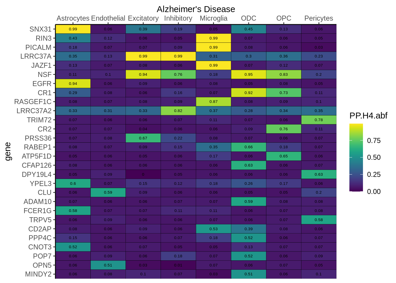

Past versions of unnamed-chunk-2-1.png

Version	Author	Date
8f071f3	Alexander Haglund	2022-11-18

Figure 2b

Figure 2c

Figure 2e

Figure 2d

FIGURE 3

The code presented here is in step 5 (Epigenetic Intersection) of the downstream results section. The basic syntax is a geom_tile() function in ggplot with colours matching cell-types. More in data/MARKDOWN/helper_funcs.r

This is only for Fig 3.a - Fig 3.c and Fig 3.d were made using the UCSC track browser.

indir<-"data/EXT_DATASETS//RESULTS/"
fig_dir<-"FIGURES/Figure_3/"

g1<-readRDS(paste0(indir,"oligo_intersect_ggobject.rds"))
g2<-readRDS(paste0(indir,"Excneuron_intersect_ggobject.rds"))
g3<-readRDS(paste0(indir,"Inneuron_intersect_ggobject.rds"))
g4<-readRDS(paste0(indir,"microglia_intersect_ggobject.rds"))

g1<-g1+theme(legend.position = "none")
g2<-g2+theme(legend.position = "none")
g3<-g3+theme(legend.position = "none")
g4<-g4+theme(legend.position = "none")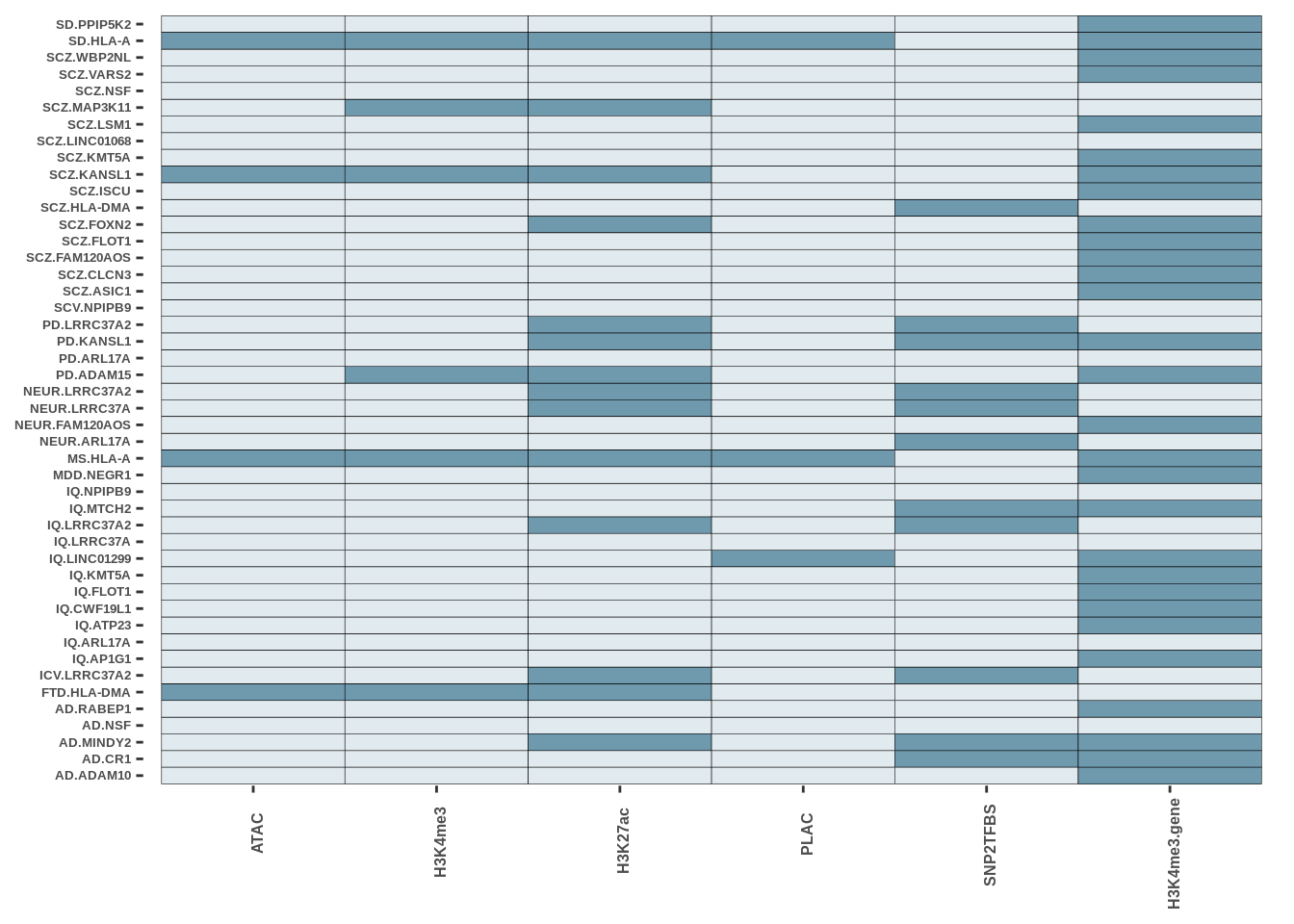

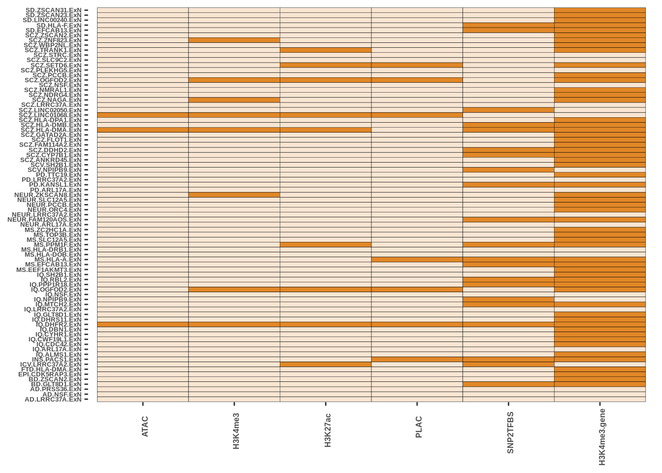
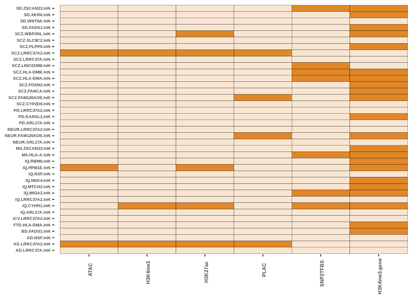
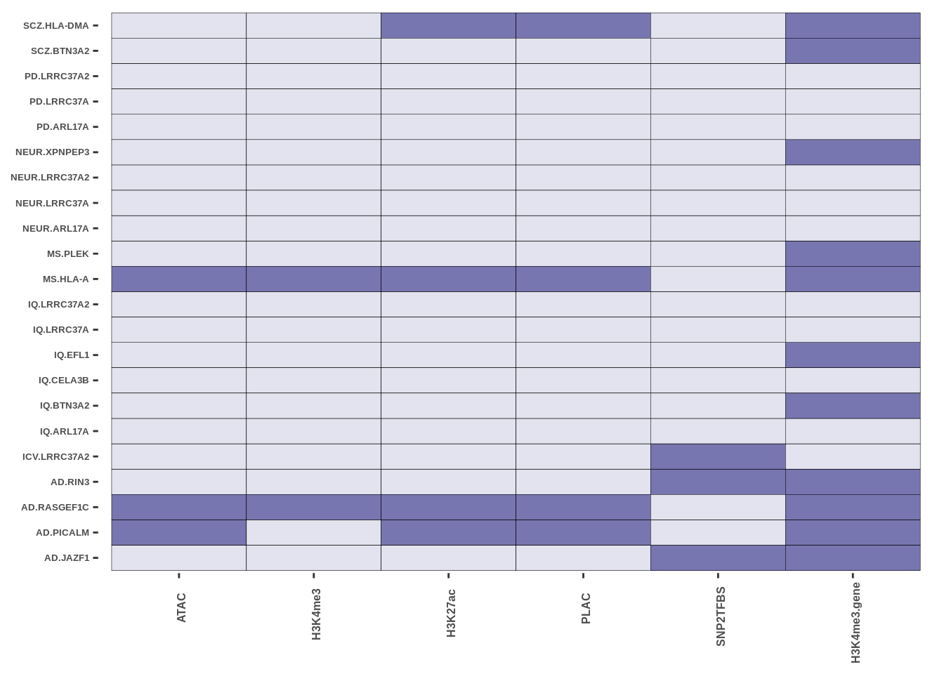
Oligo

g1

Past versions of unnamed-chunk-4-1.png

Version	Author	Date
8f071f3	Alexander Haglund	2022-11-18

ExcNeur

g2

Past versions of unnamed-chunk-5-1.png

Version	Author	Date
8f071f3	Alexander Haglund	2022-11-18

InNeur

g3

Past versions of unnamed-chunk-6-1.png

Version	Author	Date
8f071f3	Alexander Haglund	2022-11-18

Microglia

g4

Past versions of unnamed-chunk-7-1.png

Version	Author	Date
8f071f3	Alexander Haglund	2022-11-18

FIGURE 4

Figure 4a

bind data together

#bind data together

pqtl<-read.table("data/TABLES/pQTL_table.txt")
stitch<-read.table("data/TABLES//stitch_table.txt")
dgidb<-read.table("data/TABLES/dgidb_table.txt")
opentargets<-read.table("data/TABLES/OpenTargets_table.txt")
coloc<-read.table("data/COLOC_MR_RESULTS//2022-10-25_FULL_COLOC_RES.txt")
full<-read.table("data/COLOC_MR_RESULTS//2022-10-25_FULL_MR_RES.txt")
full<-full[full$IVW<0.05,]
full$trait_gene<-paste0(full$GWAS,"_",full$gene)
full$IVW_dir<-sapply(full$IVW_beta,function(x){
    if(x>0){
        return("positive")
        }else{
        return("negative")
        }
    })
direction_vector<-vector()
for(i in 1:nrow(full)){
    tmp<-full[full$trait_gene %in% full$trait_gene[i],]
    betas<-tmp$IVW_beta
    
    if(all(betas>0)==TRUE){
    dir<-"positive"
    } else if(all(betas<0)==TRUE){
    dir<-"negative"
    }else{
        dir<-"N/A"
        }
    direction_vector<-c(direction_vector,dir)    
        }
full$IVW_dir<-direction_vector    


coloc$trait_gene_ct<-paste0(coloc$GWAS,"_",coloc$gene,"_",coloc$celltype)
trait_gene_ct<-paste0(pqtl$GWAS,"_",pqtl$gene,"_",pqtl$celltype)
coloc<-coloc[match(trait_gene_ct,coloc$trait_gene_ct),]

plot_df<-data.frame(gene_trait=paste0(pqtl$GWAS,".",pqtl$gene),
                    pQTL=pqtl$pQTL_hit,
                    STITCH=stitch$STITCH_intersect,
                    DGidb=dgidb$DGIDB_intersect,
                    OpenTargets=opentargets$OpenTargets_disease_hit,
                   coloc=coloc$PP.H4.abf,
                   celltype=pqtl$celltype,
                   IVW_dir=full$IVW_dir)

prep plots

n_rows<-nrow(plot_df)
half<-round(n_rows/2)

#split in two (plot is too big otherwise)
plot_df1<-plot_df[1:half,c("gene_trait","pQTL","STITCH","DGidb","OpenTargets")]
melt_df<-melt(plot_df1,id=c("gene_trait"))
ggplot_mainplot1<-ggplot(melt_df,aes(x=variable,y=gene_trait,fill=value))+geom_tile(color="black")+
scale_fill_manual(values=c("#c8c8c8","#A6CEE3","#1F78B4"))+scale_x_discrete(expand=c(0,0))


plot_df2<-plot_df[half:n_rows,c("gene_trait","pQTL","STITCH","DGidb","OpenTargets")]
melt_df<-melt(plot_df2,id=c("gene_trait"))
ggplot_mainplot2<-ggplot(melt_df,aes(x=variable,y=gene_trait,fill=value))+geom_tile(color="black")+
scale_fill_manual(values=c("#c8c8c8","#A6CEE3","#1F78B4"))+scale_x_discrete(expand=c(0,0))



##coloc PPH4 bar
coloc_bar<-plot_df[,c("gene_trait","coloc")]

coloc_bar1<-coloc_bar[1:half,]
melt_df<-melt(coloc_bar1,id=c("gene_trait"))
ggplot_coloc1<-ggplot(melt_df,aes(x=variable,y=gene_trait,fill=value))+geom_tile(color="black")+
scale_fill_viridis(limits=c(0.5,1))

coloc_bar2<-coloc_bar[half:n_rows,]
melt_df<-melt(coloc_bar2,id=c("gene_trait"))
ggplot_coloc2<-ggplot(melt_df,aes(x=variable,y=gene_trait,fill=value))+geom_tile(color="black")+
scale_fill_viridis(limits=c(0.5,1))

##celltype MR direction

celltype_dir<-plot_df[,c("gene_trait","celltype","IVW_dir")]
celltype_dir1<-celltype_dir[1:half,]

ggplot_celltype_dir1<-ggplot(celltype_dir1,aes(x=IVW_dir,y=gene_trait,fill=celltype,group=celltype))+
geom_point(shape=22,size=2,stroke=0.1,position=position_dodge(w=0.7))+
scale_fill_manual(values = colorvec)+
theme_classic()+
geom_vline(xintercept=0,linetype="dotted")

celltype_dir2<-celltype_dir[half:n_rows,]

ggplot_celltype_dir2<-ggplot(celltype_dir2,aes(x=IVW_dir,y=gene_trait,fill=celltype,group=celltype))+
geom_point(shape=22,size=2,stroke=0.1,position=position_dodge(w=0.7))+
scale_fill_manual(values = colorvec)+
theme_classic()+
geom_vline(xintercept=0,linetype="dotted")

##direction only
ivw_dir<-plot_df[,c("gene_trait","IVW_dir")]
ivw_dir$trait<-"gwas"
ivw_dir1<-ivw_dir[1:half,]

ggplot_ivwdir1<-ggplot(ivw_dir1,aes(y=gene_trait,x=trait,fill=IVW_dir,group=IVW_dir))+geom_tile(colour="black")+
scale_fill_manual(values = c("#c8c8c8","#F8766D","#00BFC4"),guide = guide_legend(reverse = TRUE))+
theme_classic()


ivw_dir<-plot_df[,c("gene_trait","IVW_dir")]
ivw_dir$trait<-"gwas"
ivw_dir2<-ivw_dir[half:n_rows,]

ggplot_ivwdir2<-ggplot(ivw_dir2,aes(y=gene_trait,x=trait,fill=IVW_dir,group=IVW_dir))+geom_tile(colour="black")+
scale_fill_manual(values = c("#F8766D","#00BFC4"),guide = guide_legend(reverse = TRUE))+
theme_classic()



##celltype bar
celltype_bar<-plot_df[,c("gene_trait","celltype")]

celltype_bar1<-celltype_bar[1:half,]
test<-celltype_bar1 %>% 
count(gene_trait,celltype,name="count") %>% 
complete(gene_trait,celltype)
newvec<-vector()
for(i in 1:nrow(test)){
    if(is.na(test$count[i])){
        newvec<-c(newvec,NA)
        }else{
        newvec<-c(newvec,test$celltype[i])
        }
    }
test$new<-newvec
# melt_df<-melt(celltype_bar1,id=c("gene_trait"))
# df2 = celltype_bar1 %>% complete(gene_trait,celltype)
ggplot_celltype1<-ggplot(test,aes(x=celltype,y=gene_trait,fill=new))+geom_tile(color="black")+
scale_fill_manual(values=colorvec,na.value="white")

celltype_bar2<-celltype_bar[half:n_rows,]
test<-celltype_bar2 %>% 
count(gene_trait,celltype,name="count") %>% 
complete(gene_trait,celltype)
newvec<-vector()
for(i in 1:nrow(test)){
    if(is.na(test$count[i])){
        newvec<-c(newvec,NA)
        }else{
        newvec<-c(newvec,test$celltype[i])
        }
    }
test$new<-newvec
# melt_df<-melt(celltype_bar2,id=c("gene_trait"))
ggplot_celltype2<-ggplot(test,aes(x=celltype,y=gene_trait,fill=new))+geom_tile(color="black")+
scale_fill_manual(values=colorvec,na.value="white")

plot1

ggplot_mainplot1<-ggplot_mainplot1+theme_classic()+
theme(axis.text.x=element_text(size=5,face="bold",angle=45,vjust=0.8,hjust=0.8,family="Helvetica"),
      axis.text.y=element_text(size=5,face="bold",vjust=0.8,family="Helvetica"),axis.title.y=element_blank(),
      axis.line.y=element_blank(),axis.line.x=element_blank(),
      axis.title.x=element_blank(),legend.key.size=unit(0.7,"cm"),
      legend.title=element_blank(),
      legend.text=element_text(size=5),
      panel.background = element_rect(fill='transparent'),
      plot.background = element_rect(fill='transparent', color=NA),
      panel.grid.major = element_blank(), panel.grid.minor = element_blank(),
      legend.background = element_rect(fill='transparent'),
      legend.key.height= unit(0.3, 'cm'),
      legend.key.width= unit(0.2, 'cm'))#

ggplot_celltype_dir1<-ggplot_celltype_dir1+theme_classic()+
theme(axis.text.x=element_text(size=5,face="bold",angle=45,vjust=0.8,hjust=0.8,family="Helvetica"),
      axis.text.y=element_blank(),axis.title.y=element_blank(),axis.ticks.y=element_blank(),
      axis.line.y=element_blank(),axis.line.x=element_blank(),
      axis.title.x=element_blank(),legend.key.size=unit(0.7,"cm"),
      legend.position="none",panel.grid.major.y=element_line(size=0.3,colour="grey"),
      legend.text=element_text(size=5),
      panel.background = element_rect(fill='transparent'),
      plot.background = element_rect(fill='transparent', color=NA),
      legend.background = element_rect(fill='transparent'),
      legend.key.height= unit(0.3, 'cm'),
      legend.key.width= unit(0.2, 'cm'))#

ggplot_ivwdir1<-ggplot_ivwdir1+theme_classic()+
theme(axis.text.x=element_blank(),
      axis.text.y=element_blank(),axis.title.y=element_blank(),axis.ticks.y=element_blank(),
      axis.ticks.x=element_blank(),
      axis.line.y=element_blank(),axis.line.x=element_blank(),
      axis.title.x=element_blank(),legend.key.size=unit(0.7,"cm"),
      legend.text=element_text(size=5), legend.title=element_text(size=5),
      panel.background = element_rect(fill='transparent'),
      plot.background = element_rect(fill='transparent', color=NA),
      legend.background = element_rect(fill='transparent'),
      legend.key.height= unit(0.3, 'cm'),
      legend.key.width= unit(0.2, 'cm'))#

ggplot_coloc1<-ggplot_coloc1+theme_classic()+
theme(axis.text.x=element_blank(),axis.ticks.x=element_blank(),
      axis.text.y=element_blank(),axis.title.y=element_blank(),axis.ticks.y=element_blank(),
      axis.line.y=element_blank(),axis.line.x=element_blank(),
      axis.title.x=element_blank(),legend.key.size=unit(0.7,"cm"),
      legend.title=element_blank(),
      legend.text=element_text(size=5),
      panel.background = element_rect(fill='transparent'),
      plot.background = element_rect(fill='transparent', color=NA),
      panel.grid.major = element_blank(), panel.grid.minor = element_blank(),
      legend.background = element_rect(fill='transparent'),
      legend.key.height= unit(0.3, 'cm'),
      legend.key.width= unit(0.2, 'cm'))#

ggplot_celltype1<-ggplot_celltype1+theme_classic()+
theme(axis.text.x=element_text(size=5,face="bold",angle=45,vjust=0.8,hjust=0.8,family="Helvetica"),
      axis.text.y=element_blank(),axis.title.y=element_blank(),axis.ticks.y=element_blank(),
      axis.line.y=element_blank(),axis.line.x=element_blank(),
      axis.title.x=element_blank(),legend.key.size=unit(0.7,"cm"),
      legend.title=element_blank(),
      legend.text=element_text(size=5),
      panel.background = element_rect(fill='transparent'),
      plot.background = element_rect(fill='transparent', color=NA),
      legend.background = element_rect(fill='transparent'),
      legend.key.height= unit(0.3, 'cm'),
      legend.key.width= unit(0.2, 'cm'))#

coloc_legend<-get_legend(ggplot_coloc1)
ggplot_mainplot1_legend<-get_legend(ggplot_mainplot1)
celltype_legend<-get_legend(ggplot_celltype1)
ivw_dir<-get_legend(ggplot_ivwdir1)


ggplot_coloc1<-ggplot_coloc1+theme(plot.margin = unit(c(0,0,0,0), "cm"),legend.position = "none")
ggplot_ivwdir1<-ggplot_ivwdir1+theme(plot.margin = unit(c(0,0,0,0), "cm"),legend.position = "none")
ggplot_mainplot1<-ggplot_mainplot1+theme(plot.margin = unit(c(0,0,0,0), "cm"),legend.position = "none")
ggplot_celltype1<-ggplot_celltype1+theme(plot.margin = unit(c(0,0,0,0), "cm"),legend.position="none")

g<-plot_grid(ggplot_mainplot1,ggplot_celltype1,ggplot_ivwdir1, align = "h", ncol =3, rel_widths = c(0.008,0.005,0.001))
g

Past versions of unnamed-chunk-10-1.png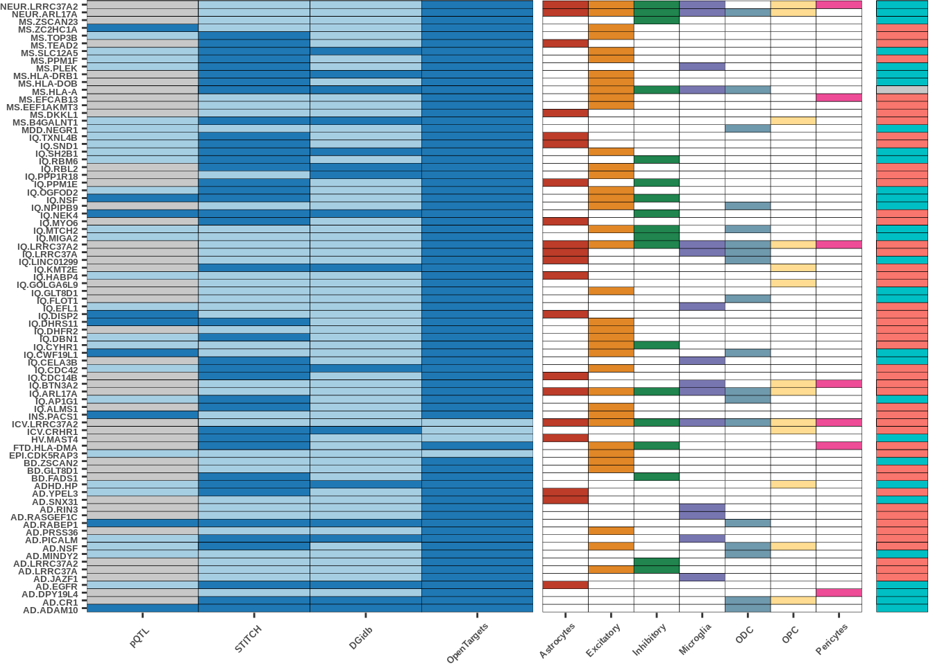

Version	Author	Date
8f071f3	Alexander Haglund	2022-11-18

plot2

ggplot_mainplot2<-ggplot_mainplot2+theme_classic()+
theme(axis.text.x=element_text(size=5,face="bold",angle=45,vjust=0.8,hjust=0.8,family="Helvetica"),
      axis.text.y=element_text(size=5,face="bold",vjust=0.8,family="Helvetica"),axis.title.y=element_blank(),
      axis.line.y=element_blank(),axis.line.x=element_blank(),
      axis.title.x=element_blank(),legend.key.size=unit(0.7,"cm"),
      legend.title=element_blank(),
      legend.text=element_text(size=5),
      panel.background = element_rect(fill='transparent'),
      plot.background = element_rect(fill='transparent', color=NA),
      panel.grid.major = element_blank(), panel.grid.minor = element_blank(),
      legend.background = element_rect(fill='transparent'),legend.box.background = element_rect(fill='transparent'))#

ggplot_coloc2<-ggplot_coloc2+theme_classic()+
theme(axis.text.x=element_blank(),axis.ticks.x=element_blank(),
      axis.text.y=element_blank(),axis.title.y=element_blank(),axis.ticks.y=element_blank(),
      axis.line.y=element_blank(),axis.line.x=element_blank(),
      axis.title.x=element_blank(),legend.key.size=unit(0.7,"cm"),
      legend.title=element_blank(),
      legend.text=element_text(size=5),
      panel.background = element_rect(fill='transparent'),
      plot.background = element_rect(fill='transparent', color=NA),
      legend.background = element_rect(fill='transparent'),legend.box.background = element_rect(fill='transparent'))#

ggplot_celltype_dir2<-ggplot_celltype_dir2+theme_classic()+
theme(axis.text.x=element_text(size=5,face="bold",angle=45,vjust=0.8,hjust=0.8,family="Helvetica"),
      axis.text.y=element_blank(),axis.title.y=element_blank(),axis.ticks.y=element_blank(),
      axis.line.y=element_blank(),axis.line.x=element_blank(),
      axis.title.x=element_blank(),legend.key.size=unit(0.7,"cm"),
      legend.position="none",panel.grid.major.y=element_line(size=0.3,colour="grey"),
      legend.text=element_text(size=5),
      panel.background = element_rect(fill='transparent'),
      plot.background = element_rect(fill='transparent', color=NA),
      legend.background = element_rect(fill='transparent'),
      legend.key.height= unit(0.3, 'cm'),
      legend.key.width= unit(0.2, 'cm'))#

ggplot_ivwdir2<-ggplot_ivwdir2+theme_classic()+
theme(axis.text.x=element_blank(),
      axis.text.y=element_blank(),axis.title.y=element_blank(),axis.ticks.y=element_blank(),
      axis.ticks.x=element_blank(),
      axis.line.y=element_blank(),axis.line.x=element_blank(),
      axis.title.x=element_blank(),legend.key.size=unit(0.7,"cm"),
      legend.text=element_text(size=5), legend.title=element_text(size=5),
      panel.background = element_rect(fill='transparent'),
      plot.background = element_rect(fill='transparent', color=NA),
      legend.background = element_rect(fill='transparent'),
      legend.key.height= unit(0.3, 'cm'),
      legend.key.width= unit(0.2, 'cm'))#

ggplot_celltype2<-ggplot_celltype2+theme_classic()+
theme(axis.text.x=element_text(size=5,face="bold",angle=45,vjust=0.8,hjust=0.8,family="Helvetica"),
      axis.text.y=element_blank(),axis.title.y=element_blank(),axis.ticks.y=element_blank(),
      axis.line.y=element_blank(),axis.line.x=element_blank(),
      axis.title.x=element_blank(),legend.key.size=unit(0.7,"cm"),
      legend.title=element_blank(),
      legend.text=element_text(size=5),
      panel.background = element_rect(fill='transparent'),
      plot.background = element_rect(fill='transparent', color=NA),
      panel.grid.major = element_blank(), panel.grid.minor = element_blank(),
      legend.background = element_rect(fill='transparent'),legend.box.background = element_rect(fill='transparent'))#

ggplot_coloc2<-ggplot_coloc2+theme(plot.margin = unit(c(0,0,0,0), "cm"),legend.position = "none")
ggplot_ivwdir2<-ggplot_ivwdir2+theme(plot.margin = unit(c(0,0,0,0), "cm"),legend.position = "none")
ggplot_mainplot2<-ggplot_mainplot2+theme(plot.margin = unit(c(0,0,0,0), "cm"),legend.position = "none")
ggplot_celltype2<-ggplot_celltype2+theme(plot.margin = unit(c(0,0,0,0), "cm"),legend.position="none")


g<-plot_grid(ggplot_mainplot2,ggplot_celltype2,ggplot_ivwdir2, align = "h", ncol =3, rel_widths = c(0.008,0.005,0.001))
g

Past versions of unnamed-chunk-11-1.png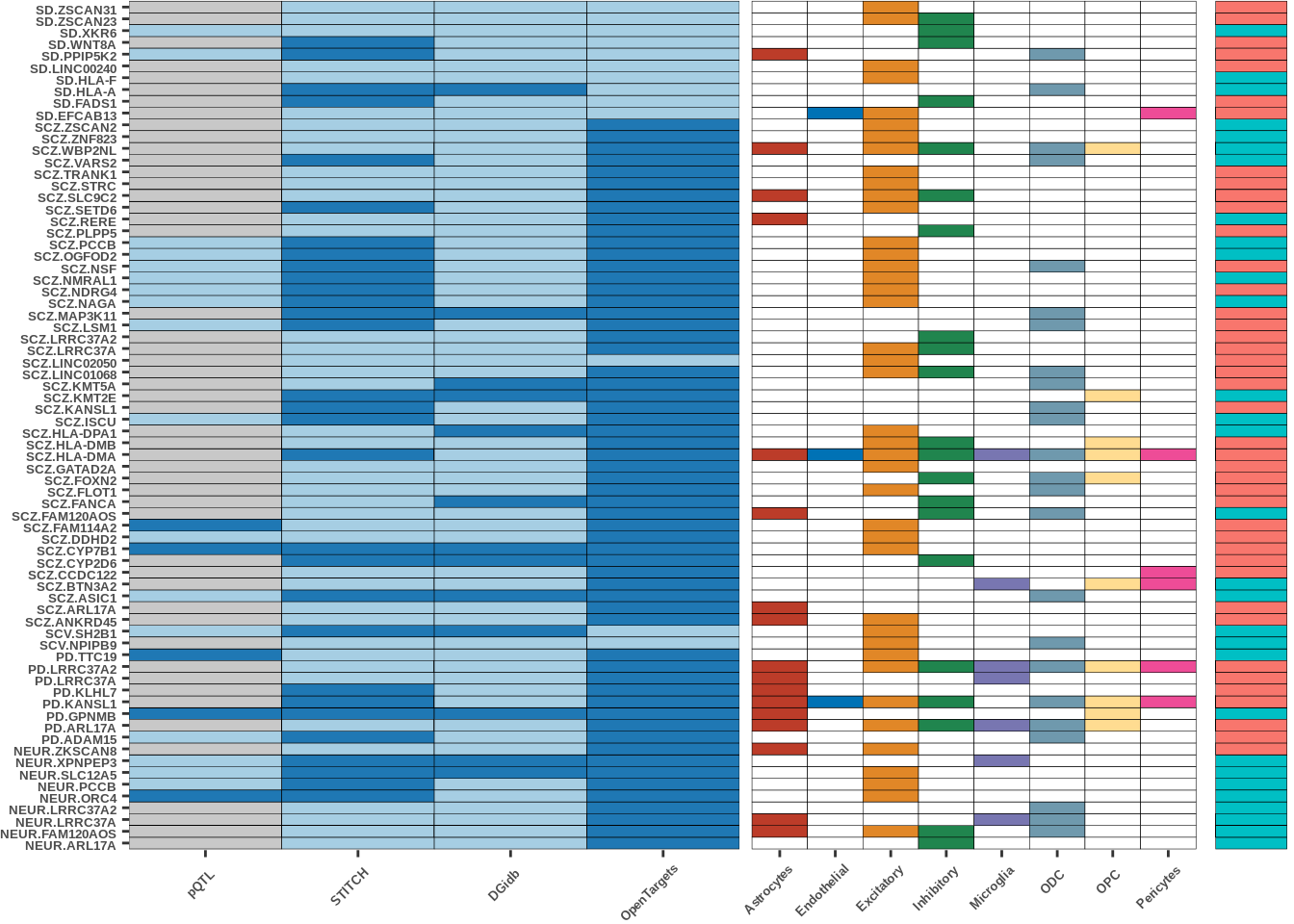

Version	Author	Date
8f071f3	Alexander Haglund	2022-11-18

FIGURE 5

Figure 5a

full<-read.table("data/COLOC_MR_RESULTS//2022-10-25_FULL_MR_RES.txt")
full<-full[full$IVW<0.05,]
full$trait_gene<-paste0(full$GWAS,"_",full$gene)
full$IVW_dir<-sapply(full$IVW_beta,function(x){
    if(x>0){
        return("CAUSAL")
        }else{
        return("PROTECTIVE")
        }
    })

tmp<-full[full$GWAS=="AD",]
tmp<-tmp[order(tmp$celltype),]
tmp$gene<-factor(tmp$gene,levels=unique(tmp$gene))
color_pal=ggsci::pal_nejm("default")(8)
colorvec<-c(Astrocytes=color_pal[1],
           Endothelial=color_pal[2],
           Excitatory=color_pal[3],
           Inhibitory=color_pal[4],Microglia=color_pal[5],
           ODC=color_pal[6],OPC=color_pal[7],Pericytes=color_pal[8])

g<-ggplot(tmp,aes(y=gene,x=IVW_beta,fill=celltype))+
geom_point(colour="black",shape=21,stroke=0.3,size=2)+
scale_fill_manual(values = colorvec)+
theme_classic()+
geom_vline(xintercept=0,linetype="dotted")+scale_x_continuous(limits=c(-0.6,0.6))
g2<-g+
theme(text=element_text(family="Helvetica",size=5),legend.text = element_text(family="Helvetica",size=5,face="bold"),
      legend.title=element_blank(),
      legend.spacing.y = unit(-1, 'cm'),axis.text.y=element_text(family="Helvetica",size=5,face="bold"))+guides(fill = guide_legend(byrow = TRUE))
g2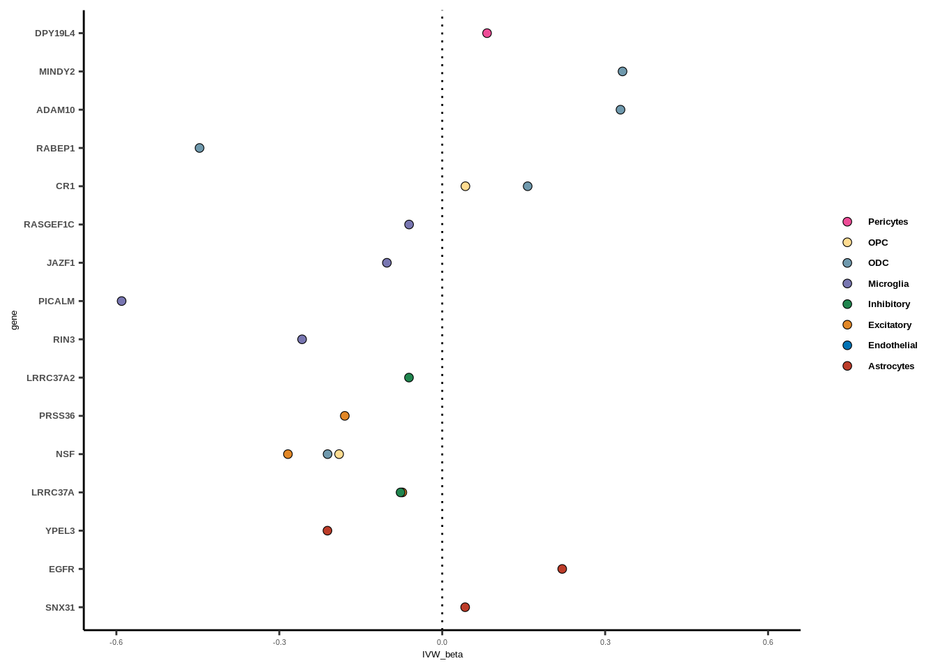

Past versions of unnamed-chunk-12-1.png

Version	Author	Date
8f071f3	Alexander Haglund	2022-11-18

Figure 5b

full<-read.table("data/COLOC_MR_RESULTS//2022-10-25_FULL_MR_RES.txt")
plot_df<-data.frame()
for(i in 1:length(unique(full$GWAS))){
    gwas<-unique(full$GWAS)[i]
    tmp_full<-full[full$GWAS==gwas,]
    cellvec<-as.vector(table(tmp_full$celltype))
    plot_df<-rbind(plot_df,data.frame(gwas=gwas,
                                      celltype=names(table(tmp_full$celltype)),
                                      occurrence=cellvec))
    }
g<-ggplot(data=plot_df,aes(y=occurrence,x=gwas,fill=celltype))+
geom_bar(stat="identity",colour="black",size=0.25)+
scale_fill_manual(values=color_pal)+theme_classic()+
geom_text(aes(label=occurrence),family="Helvetica",size=5*0.36, position = position_stack(vjust = 0.5))+
theme_classic()+scale_y_continuous(expand=c(0,0))+
labs(title="Cell-type proportions in MR results",size=7,family="Helvetica")+
theme(text=element_text(size=7,family="Helvetica"),axis.text.x=element_text(size=5,face="bold",angle=90),
                                  axis.text.y=element_text(size=5),
                                  axis.title.y=element_blank(),
                                 axis.title.x=element_blank(),legend.position="none",
     title=element_text(size=7,face="bold"))
g

Past versions of unnamed-chunk-13-1.png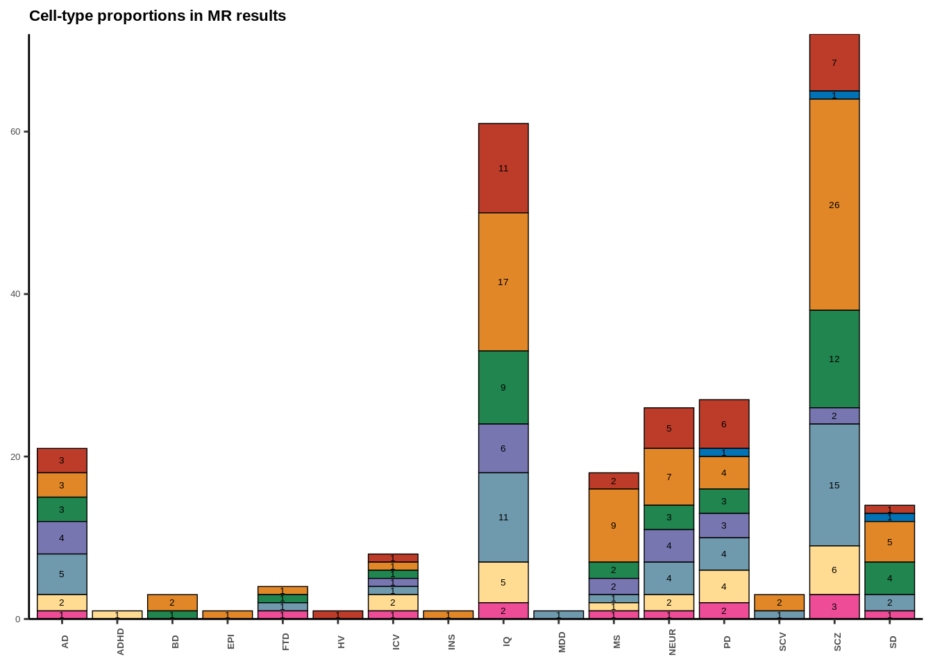

Version	Author	Date
8f071f3	Alexander Haglund	2022-11-18

Figure 5c

full<-read.table("data/COLOC_MR_RESULTS//2022-10-25_FULL_MR_RES.txt")
full$celltype_gene<-paste0(full$celltype,".",full$gene)
scz<-full[full$GWAS=="SCZ",]
iq<-full[full$GWAS=="IQ",]
common<-intersect(iq$celltype_gene,scz$celltype_gene)

##remove ct/gene combinations in other traits - we are only interested in the SCZ/IQ overlap
# filtered<-full[full$celltype_gene %in% common,]
# filtered<-filtered[!filtered$GWAS %in% c("SCZ","IQ"),]
# to_exclude<-unique(filtered$celltype_gene)
# common<-common[!common %in% to_exclude]



#filter both
scz<-scz[match(common,scz$celltype_gene),]
iq<-iq[match(common,iq$celltype_gene),]
df<-data.frame(celltype_gene=common,IQ=iq$IVW_beta,SCZ=scz$IVW_beta)


##now plot
ylims=c(-0.2,0.2)
xlims=c(-0.7,0.7)

g<-ggplot(df,aes(x=SCZ,y=IQ,fill=celltype_gene))+
geom_point(shape=21,size=2)+
scale_y_continuous(limits=ylims)+
scale_x_continuous(limits=xlims)+
geom_vline(xintercept =0,linetype="dotted")+
geom_hline(yintercept =0,linetype="dotted")+theme_classic()+
theme(text=element_text(size=5,family="Helvetica"),legend.title=element_blank(),legend.text = element_text(family="Helvetica",size=5,face="bold"),legend.spacing.y = unit(-1, 'cm'))+
xlab("SCZ - MR beta")+ylab("IQ - MR beta")+
guides(fill = guide_legend(byrow = TRUE))
g

Past versions of unnamed-chunk-14-1.png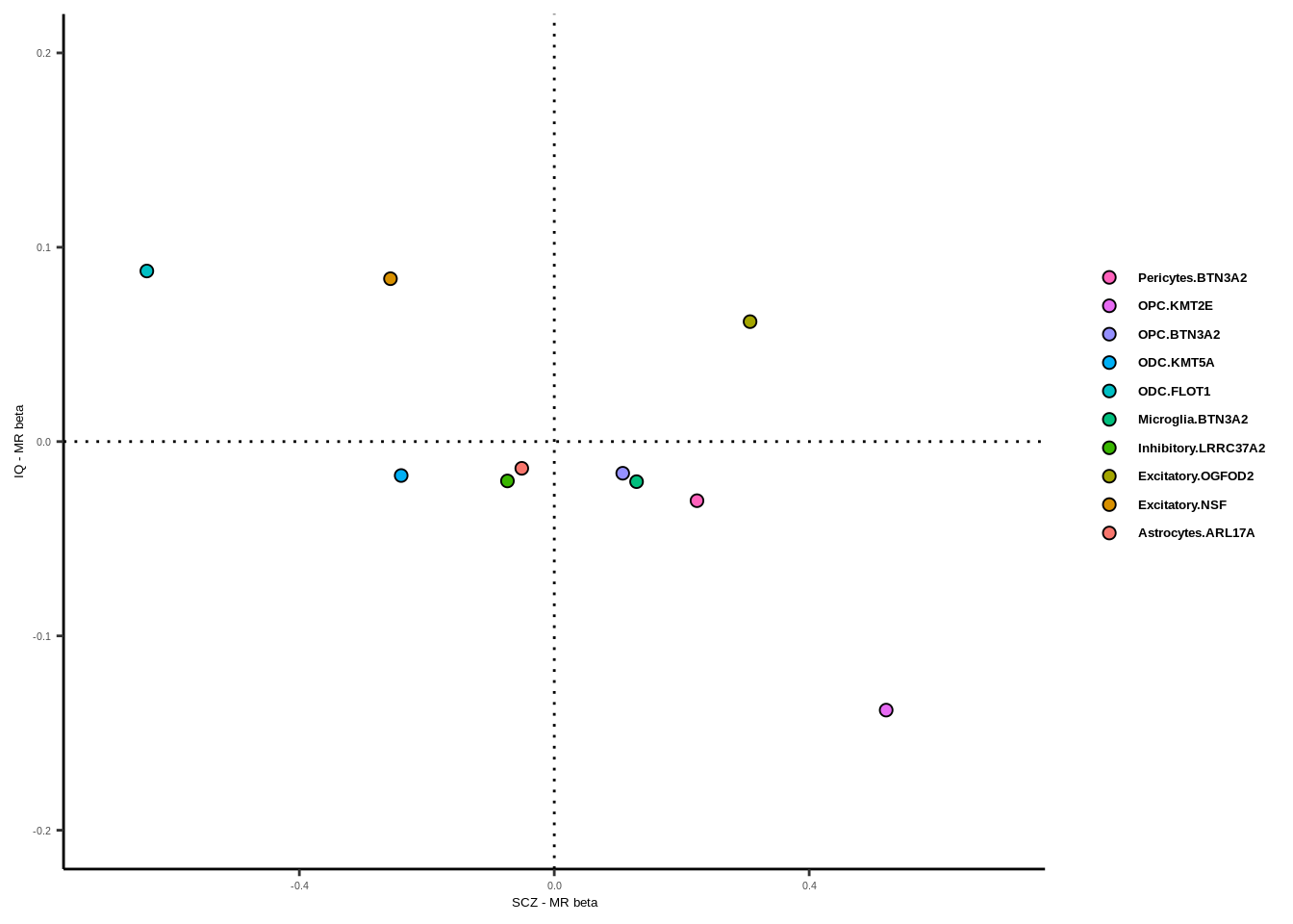

Version	Author	Date
8f071f3	Alexander Haglund	2022-11-18

Figure 5d

full<-read.table("data/COLOC_MR_RESULTS//2022-10-25_FULL_MR_RES.txt")
full$celltype_gene<-paste0(full$celltype,".",full$gene)
scz<-full[full$GWAS=="SCZ",]
neur<-full[full$GWAS=="NEUR",]
common<-intersect(neur$celltype_gene,scz$celltype_gene)

# filtered<-full[full$celltype_gene %in% common,]
# filtered<-filtered[!filtered$GWAS %in% c("SCZ","NEUR"),]
# to_exclude<-unique(filtered$celltype_gene)
# common<-common[!common %in% to_exclude]


#filter both
scz<-scz[match(common,scz$celltype_gene),]
neur<-neur[match(common,neur$celltype_gene),]
df<-data.frame(celltype_gene=common,NEUR=neur$IVW_beta,SCZ=scz$IVW_beta)


##now plot
ylims=c(-0.2,0.2)
xlims=c(-0.8,0.8)

g<-ggplot(df,aes(x=SCZ,y=NEUR,fill=celltype_gene))+
geom_point(shape=21,size=2)+
scale_y_continuous(limits=ylims)+
scale_x_continuous(limits=xlims)+
geom_vline(xintercept =0,linetype="dotted")+
geom_hline(yintercept =0,linetype="dotted")+theme_classic()+
theme(text=element_text(size=5,family="Helvetica"),legend.text = element_text(family="Helvetica",size=5,face="bold"),legend.title=element_blank(),legend.spacing.y = unit(-1, 'cm'))+
xlab("SCZ - MR beta")+ylab("NEUR - MR beta")+guides(fill = guide_legend(byrow = TRUE))
g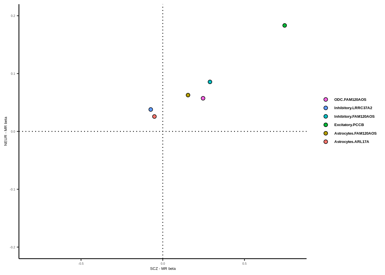

Past versions of unnamed-chunk-15-1.png

Version	Author	Date
8f071f3	Alexander Haglund	2022-11-18

Session information

sessionInfo()

R version 4.0.5 (2021-03-31)
Platform: x86_64-conda-linux-gnu (64-bit)
Running under: Ubuntu 18.04.6 LTS

Matrix products: default
BLAS/LAPACK: /home/ah3918/anaconda3/envs/ODIN3/lib/libopenblasp-r0.3.12.so

locale:
 [1] LC_CTYPE=en_GB.UTF-8       LC_NUMERIC=C              
 [3] LC_TIME=en_GB.UTF-8        LC_COLLATE=en_GB.UTF-8    
 [5] LC_MONETARY=en_GB.UTF-8    LC_MESSAGES=en_GB.UTF-8   
 [7] LC_PAPER=en_GB.UTF-8       LC_NAME=C                 
 [9] LC_ADDRESS=C               LC_TELEPHONE=C            
[11] LC_MEASUREMENT=en_GB.UTF-8 LC_IDENTIFICATION=C       

attached base packages:
[1] grid      stats     graphics  grDevices utils     datasets  methods  
[8] base     

other attached packages:
[1] reshape_0.8.9     tidyr_1.2.1       cowplot_1.1.1     dplyr_1.0.9      
[5] ggsci_2.9         viridis_0.6.2     viridisLite_0.4.1 ggplot2_3.3.6    
[9] workflowr_1.7.0  

loaded via a namespace (and not attached):
 [1] tidyselect_1.1.2 xfun_0.32        bslib_0.4.0      purrr_0.3.4     
 [5] colorspace_2.0-3 vctrs_0.5.0      generics_0.1.3   htmltools_0.5.3 
 [9] yaml_2.3.5       utf8_1.2.2       rlang_1.0.6      jquerylib_0.1.4 
[13] later_1.2.0      pillar_1.8.1     glue_1.6.2       withr_2.5.0     
[17] DBI_1.1.3        plyr_1.8.7       lifecycle_1.0.3  stringr_1.4.0   
[21] munsell_0.5.0    gtable_0.3.1     evaluate_0.16    labeling_0.4.2  
[25] knitr_1.39       callr_3.7.1      fastmap_1.1.0    httpuv_1.6.5    
[29] ps_1.7.1         fansi_1.0.3      highr_0.9        Rcpp_1.0.9      
[33] promises_1.2.0.1 scales_1.2.1     cachem_1.0.6     jsonlite_1.8.0  
[37] farver_2.1.1     fs_1.5.2         gridExtra_2.3    digest_0.6.30   
[41] stringi_1.7.8    processx_3.7.0   getPass_0.2-2    rprojroot_2.0.3 
[45] cli_3.4.1        tools_4.0.5      magrittr_2.0.3   sass_0.4.2      
[49] tibble_3.1.8     whisker_0.4      pkgconfig_2.0.3  ellipsis_0.3.2  
[53] assertthat_0.2.1 rmarkdown_2.15   httr_1.4.3       rstudioapi_0.13 
[57] R6_2.5.1         git2r_0.30.1     compiler_4.0.5