Binarized Data Logistic Regression
Sarah E Taylor
2024-02-13
Last updated: 2024-02-13
Checks: 5 2
Knit directory: LocksofLineage/
This reproducible R Markdown analysis was created with workflowr (version 1.7.1). The Checks tab describes the reproducibility checks that were applied when the results were created. The Past versions tab lists the development history.
The R Markdown is untracked by Git. To know which version of the R
Markdown file created these results, you’ll want to first commit it to
the Git repo. If you’re still working on the analysis, you can ignore
this warning. When you’re finished, you can run
wflow_publish to commit the R Markdown file and build the
HTML.
Great job! The global environment was empty. Objects defined in the global environment can affect the analysis in your R Markdown file in unknown ways. For reproduciblity it’s best to always run the code in an empty environment.
The command set.seed(20231117) was run prior to running
the code in the R Markdown file. Setting a seed ensures that any results
that rely on randomness, e.g. subsampling or permutations, are
reproducible.
Great job! Recording the operating system, R version, and package versions is critical for reproducibility.
Nice! There were no cached chunks for this analysis, so you can be confident that you successfully produced the results during this run.
Using absolute paths to the files within your workflowr project makes it difficult for you and others to run your code on a different machine. Change the absolute path(s) below to the suggested relative path(s) to make your code more reproducible.
| absolute | relative |
|---|---|
| ~/GitHub/LocksofLineage/analysis/binarized_phylogenetic_logistic_regression_function.R | analysis/binarized_phylogenetic_logistic_regression_function.R |
| ~/GitHub/LocksofLineage/data/data_binarized_Feb13.csv | data/data_binarized_Feb13.csv |
| ~/GitHub/LocksofLineage/data/Phylo_Project_Data/MamPhy_BDvr_Completed_v2_tree0000.tre | data/Phylo_Project_Data/MamPhy_BDvr_Completed_v2_tree0000.tre |
Great! You are using Git for version control. Tracking code development and connecting the code version to the results is critical for reproducibility.
The results in this page were generated with repository version 9ac420b. See the Past versions tab to see a history of the changes made to the R Markdown and HTML files.
Note that you need to be careful to ensure that all relevant files for
the analysis have been committed to Git prior to generating the results
(you can use wflow_publish or
wflow_git_commit). workflowr only checks the R Markdown
file, but you know if there are other scripts or data files that it
depends on. Below is the status of the Git repository when the results
were generated:
Ignored files:
    Ignored:    .DS_Store
    Ignored:    .Rhistory
    Ignored:    .Rproj.user/
    Ignored:    data/.DS_Store

Untracked files:
    Untracked:  analysis/binarized_logistic_regression.Rmd
    Untracked:  analysis/binarized_phylogenetic_logistic_regression_function.R
    Untracked:  data/data_binarized_Feb13.csv

Unstaged changes:
    Modified:   analysis/Dimorphism_on_the_Head.Rmd
    Modified:   analysis/expanded_trait_data.Rmd
    Modified:   analysis/logistic_regression_function_script.Rmd
Note that any generated files, e.g. HTML, png, CSS, etc., are not included in this status report because it is ok for generated content to have uncommitted changes.
There are no past versions. Publish this analysis with
wflow_publish() to start tracking its development.
Logistic Regression Model Creation
prerequisite_mapping <- list(
  ConM = "Natal_Coat",
  ConB = "Natal_Coat",
  ConD = "Natal_Coat",
  incon = "Natal_Coat",
  SD_Location_Head = "Sexual_Dimorphism",
  Direction_Male = "Sexual_Dimorphism",
  Darker_Male = "Sexual_Dichromatism"
)
# Load the custom function
source("~/GitHub/LocksofLineage/analysis/binarized_phylogenetic_logistic_regression_function.R")
# Load your dataset
data_file_path <- "~/GitHub/LocksofLineage/data/data_binarized_Feb13.csv"
primate_data <- read_csv(data_file_path)
tree_file_path <- "~/GitHub/LocksofLineage/data/Phylo_Project_Data/MamPhy_BDvr_Completed_v2_tree0000.tre"
# List all variable names (excluding species name if it's there)
variable_names <- colnames(primate_data)[!colnames(primate_data) %in% c("family", "Genus", "species")]
# Initialize a list (or another structure) to store summaries or results
model_results_binarized_prereq <- list()
# Loop over all variable combinations
for (outcome_var in variable_names) {
for (predictor_var in variable_names) {
if (outcome_var != predictor_var) {
#Check if the current predictor_var has a prerequisite
prerequisite_trait <- ifelse(predictor_var %in% names(prerequisite_mapping), prerequisite_mapping[[predictor_var]], "")
# Run the phylogenetic logistic regression analysis
model_summary_binarized_prereq <- run_binarized_phylogenetic_logistic_regression(outcome_var, predictor_var, tree_file_path, data_file_path)
if(!exists("model_results_binarized_prereq")) {
model_results_binarized_prereq <- list()
}
# Store the summary with a meaningful identifier
model_id <- paste(outcome_var, "vs", predictor_var, sep = "_")
model_results_binarized_prereq[[model_id]] <- model_summary_binarized_prereq
# Optionally, print or inspect the summary
print(model_summary_binarized_prereq)
}
}
}Analyzing the Models
# Initialize the association matrix with the correct dimensions and names
n_variables <- length(variable_names)
association_matrix <- matrix(NA, nrow = n_variables, ncol = n_variables, dimnames = list(variable_names, variable_names))

# Loop over model_results to extract and store coefficients
for (model_id in names(model_results_binarized_prereq)) {
  model_summary_binarized_prereq <- model_results_binarized_prereq[[model_id]]

  if (!is.null(model_summary_binarized_prereq) && "summary.phyloglm" %in% class(model_summary_binarized_prereq)) {
    # Extract coefficients matrix
    coefficients_matrix <- model_summary_binarized_prereq$coefficients

    # Assuming you're interested in the first predictor's coefficient
    # and that predictor variable names directly match those in variable_names
    predictor_name <- gsub(".*vs_", "", model_id)  # Extract predictor variable name from model_id
    if (predictor_name %in% rownames(coefficients_matrix)) {
      coefficient <- coefficients_matrix[predictor_name, "Estimate"]

      # Determine indices for the association matrix based on variable names
      outcome_var <- gsub("_vs.*", "", model_id)  # Extract outcome variable name from model_id
      i <- which(variable_names == outcome_var)
      j <- which(variable_names == predictor_name)

      # Populate the association matrix
      if (length(i) == 1 && length(j) == 1) {  # Ensure valid indices
        association_matrix[i, j] <- coefficient
      }
    }
  }
}

# Now, the association matrix should be populated with the coefficients
# Assuming `model_results` is a list where each element is a model summary including AIC
# Extract AIC values and model identifiers
aic_values <- sapply(model_results_binarized_prereq, function(summary) summary$aic)
# Adjust extraction based on your summary structure
model_ids <- names(model_results_binarized_prereq)
# Combine into a data frame for easy sorting and viewing
aic_df <- data.frame(model_id = model_ids, AIC = aic_values)
# Sort by AIC values
aic_sorted <- aic_df[order(aic_df$AIC), ]
# View sorted models by AIC
#print(aic_sorted)
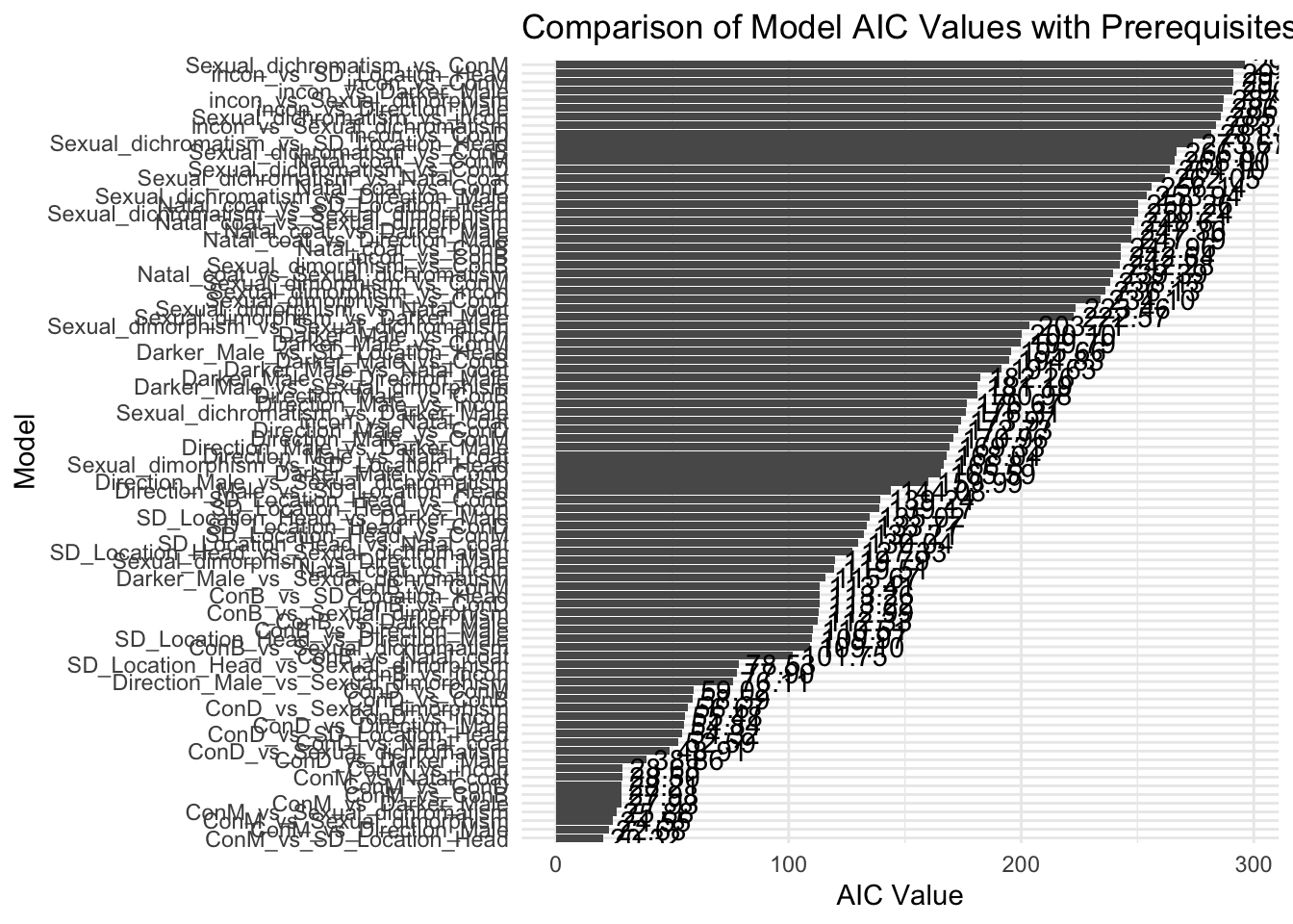
# Identify best models (e.g., top 5 models with lowest AIC)
best_models <- head(aic_sorted, 5)
print(best_models) model_id AIC
ConM_vs_SD_Location_Head ConM_vs_SD_Location_Head 20.32009
ConM_vs_Direction_Male ConM_vs_Direction_Male 22.68275
ConM_vs_Sexual_dimorphism ConM_vs_Sexual_dimorphism 24.54911
ConM_vs_Sexual_dichromatism ConM_vs_Sexual_dichromatism 25.87730
ConM_vs_Darker_Male ConM_vs_Darker_Male 27.92916# Create the plot for AIC of models with prerequisites
ggplot(aic_sorted, aes(x = reorder(model_id, AIC), y = AIC)) +
geom_bar(stat = "identity") +
theme_minimal() +
coord_flip() + # Flip coordinates to make the plot horizontal; easier to read model names
labs(x = "Model", y = "AIC Value", title = "Comparison of Model AIC Values with Prerequisites") +
geom_text(aes(label = sprintf("%.2f", AIC), hjust = -0.1)) # Add AIC values as text labels
#Basic r plotting
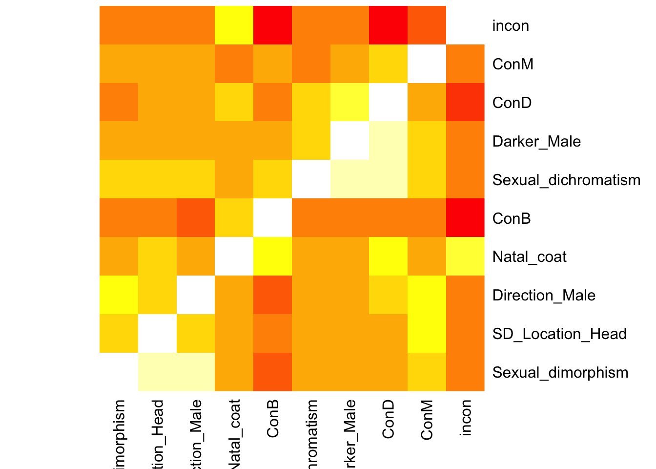
heatmap(association_matrix, Rowv = NA, Colv = NA, col = heat.colors(10), scale = "none")
sessionInfo()R version 4.2.1 (2022-06-23)
Platform: x86_64-apple-darwin17.0 (64-bit)
Running under: macOS Big Sur ... 10.16
Matrix products: default
BLAS: /Library/Frameworks/R.framework/Versions/4.2/Resources/lib/libRblas.0.dylib
LAPACK: /Library/Frameworks/R.framework/Versions/4.2/Resources/lib/libRlapack.dylib
locale:
[1] en_US.UTF-8/en_US.UTF-8/en_US.UTF-8/C/en_US.UTF-8/en_US.UTF-8
attached base packages:
[1] stats graphics grDevices utils datasets methods base
other attached packages:
[1] lubridate_1.9.2 forcats_1.0.0 stringr_1.5.0 dplyr_1.1.0
[5] purrr_1.0.1 readr_2.1.4 tidyr_1.3.0 tibble_3.1.8
[9] ggplot2_3.4.4 tidyverse_2.0.0 phylolm_2.6.2 ape_5.7
loaded via a namespace (and not attached):
[1] Rcpp_1.0.11 lattice_0.20-45 listenv_0.9.0
[4] rprojroot_2.0.4 digest_0.6.30 utf8_1.2.2
[7] parallelly_1.36.0 R6_2.5.1 evaluate_0.23
[10] highr_0.10 pillar_1.8.1 rlang_1.1.2
[13] rstudioapi_0.14 jquerylib_0.1.4 rmarkdown_2.20
[16] labeling_0.4.2 bit_4.0.5 munsell_0.5.0
[19] compiler_4.2.1 httpuv_1.6.11 xfun_0.41
[22] pkgconfig_2.0.3 globals_0.16.2 htmltools_0.5.4
[25] tidyselect_1.2.0 workflowr_1.7.1 codetools_0.2-18
[28] fansi_1.0.3 future_1.33.0 crayon_1.5.2
[31] tzdb_0.3.0 withr_2.5.0 later_1.3.1
[34] grid_4.2.1 nlme_3.1-160 jsonlite_1.8.8
[37] gtable_0.3.1 lifecycle_1.0.3 git2r_0.32.0
[40] magrittr_2.0.3 scales_1.2.1 vroom_1.6.1
[43] future.apply_1.11.0 cli_3.6.2 stringi_1.7.8
[46] cachem_1.0.6 farver_2.1.1 fs_1.6.1
[49] promises_1.2.1 bslib_0.4.2 ellipsis_0.3.2
[52] vctrs_0.5.2 generics_0.1.3 tools_4.2.1
[55] bit64_4.0.5 glue_1.6.2 hms_1.1.2
[58] parallel_4.2.1 fastmap_1.1.0 yaml_2.3.7
[61] timechange_0.2.0 colorspace_2.0-3 knitr_1.42
[64] sass_0.4.5