epistasis
aluetge
2019-07-26
Last updated: 2019-11-19
Checks: 7 0
Knit directory: transcriptome_cll/
This reproducible R Markdown analysis was created with workflowr (version 1.4.0). The Checks tab describes the reproducibility checks that were applied when the results were created. The Past versions tab lists the development history.
Great! Since the R Markdown file has been committed to the Git repository, you know the exact version of the code that produced these results.
Great job! The global environment was empty. Objects defined in the global environment can affect the analysis in your R Markdown file in unknown ways. For reproduciblity it’s best to always run the code in an empty environment.
The command set.seed(20190511) was run prior to running the code in the R Markdown file. Setting a seed ensures that any results that rely on randomness, e.g. subsampling or permutations, are reproducible.
Great job! Recording the operating system, R version, and package versions is critical for reproducibility.
Nice! There were no cached chunks for this analysis, so you can be confident that you successfully produced the results during this run.
Great job! Using relative paths to the files within your workflowr project makes it easier to run your code on other machines.
Great! You are using Git for version control. Tracking code development and connecting the code version to the results is critical for reproducibility. The version displayed above was the version of the Git repository at the time these results were generated.
Note that you need to be careful to ensure that all relevant files for the analysis have been committed to Git prior to generating the results (you can use wflow_publish or wflow_git_commit). workflowr only checks the R Markdown file, but you know if there are other scripts or data files that it depends on. Below is the status of the Git repository when the results were generated:
Ignored files:
    Ignored:    .Rhistory
    Ignored:    .Rproj.user/

Untracked files:
    Untracked:  data/2018-03-05_IGHV.RData
    Untracked:  data/patmeta_170324.RData
    Untracked:  output/IGHV1_69.svg
    Untracked:  output/cluster1000exprgenes.pdf
    Untracked:  output/cluster500exprgenes.pdf
    Untracked:  output/desRes_15112019.RData
    Untracked:  output/figures/hist_mutations.svg
    Untracked:  output/figures/overview_mutations.pdf
    Untracked:  output/figures/paper_fig/
    Untracked:  output/figures/r_objects/
    Untracked:  output/figures/sum_diffGenes_0.05_2.pdf
    Untracked:  output/figures/sum_diffGenes_noTsig.pdf
    Untracked:  output/figures/sum_diffGenes_noTsig_IGHVTri12.pdf

Unstaged changes:
    Modified:   analysis/IGHV.Rmd
    Modified:   analysis/Notch1.Rmd
    Modified:   analysis/TP53.Rmd
    Modified:   analysis/trisomy12.Rmd
    Modified:   output/diff_genes/ATM_diffGenes.csv
    Modified:   output/diff_genes/BRAF_diffGenes.csv
    Modified:   output/diff_genes/MED12_diffGenes.csv
    Modified:   output/diff_genes/NOTCH1_diffGenes.csv
    Modified:   output/diff_genes/SF3B1_diffGenes.csv
    Modified:   output/diff_genes/TP53_diffGenes.csv
    Modified:   output/diff_genes/del11q22.3_diffGenes.csv
    Modified:   output/diff_genes/del13q14_diffGenes.csv
    Modified:   output/diff_genes/del17p13_diffGenes.csv
    Modified:   output/diff_genes/del8p12_diffGenes.csv
    Modified:   output/diff_genes/gain8q24_diffGenes.csv
    Modified:   output/diff_genes/trisomy12_diffGenes.csv
    Modified:   output/figures/pca_Meth_top150.svg
Note that any generated files, e.g. HTML, png, CSS, etc., are not included in this status report because it is ok for generated content to have uncommitted changes.
These are the previous versions of the R Markdown and HTML files. If you’ve configured a remote Git repository (see ?wflow_git_remote), click on the hyperlinks in the table below to view them.
| File | Version | Author | Date | Message |
|---|---|---|---|---|
| Rmd | a132f77 | aluetge | 2019-11-19 | wflow_publish(c(“analysis/epistasis.Rmd”, “analysis/Gain8q24.Rmd”, “analysis/general_eda.Rmd”, “analysis/Med12.Rmd”)) |
| html | 2cd07c0 | aluetge | 2019-11-17 | Build site. |
| Rmd | d607508 | aluetge | 2019-11-17 | wflow_publish(c(“analysis/epistasis.Rmd”)) |
| html | cc24f92 | aluetge | 2019-07-28 | Build site. |
Epistasis in CLL
We find correlation and coexpression of several muatations and genetic variants in CLL. How is this reflected on the transcriptome level? Is there a connection?
IGHV and Trisomy12
IGHV and trisomy12 are the most severe genomic modification on transcriptome level. How do they affect each other?
load packages
library(Biobase)
library(ggplot2)
library(genefilter)
library(DESeq2)
library(gridExtra)
library(reshape2)
library(dplyr)
library(geneplotter)
library(RColorBrewer)
library(ComplexHeatmap)
library(circlize)
library(piano)
library(ggpubr)
library(here)
load datasets
data_dir <- here("data")
output_dir <- here("output")
figure_dir <- here("output/figures")

#Countdata
load(paste0(data_dir, "/ddsrnaCLL_150218.RData"))
Epistasis model
Use deseq2 to determine genes, which can be described by epistatisc interactions (focus on trisomy12 and IGHV)
###Deseq
ddsCLL <- estimateSizeFactors(ddsCLL)

#exclude NAs
ddsCLL <- ddsCLL[,!is.na(colData(ddsCLL)[,"IGHV"])]
ddsCLL <- ddsCLL[,!is.na(colData(ddsCLL)[,"trisomy12"])]

RNAnorm <- varianceStabilizingTransformation(ddsCLL, blind=T)
colnames(RNAnorm) <- colData(RNAnorm)$PatID

#design matrix with interaction term
design(ddsCLL) <- as.formula(paste("~ IGHV + trisomy12 + IGHV:trisomy12"))
#rnaRaw <- DESeq(ddsCLL, betaPrior = FALSE)
#resultsNames(rnaRaw)
#res <- results(rnaRaw, name = "IGHVU.trisomy121")

#saveRDS(res, paste0(output_dir, "/res_epistatsis_ighv_tri12.rds"))
res <- readRDS(paste0(output_dir, "/res_epistatsis_ighv_tri12.rds"))

resOrdered <- res[order(res$pvalue),]
resOrderedTab <- as.data.frame(resOrdered)
resOrderedTab$symbol <- rowData(RNAnorm[rownames(resOrdered),])$symbol

resSig <- subset(resOrdered, padj < 0.1)# & abs(log2FoldChange) > 2)
resTab <- as.data.frame(resSig)
resTab$symbol <- rowData(RNAnorm[rownames(resSig),])$symbol
Gene expression of epistatic genes
Heatmap of interacting genes
  #filter by variant
  sig_Genes <- rownames(resSig)

  #gene expression data
  geneExpression = assay(RNAnorm)[sig_Genes,]
  rownames(geneExpression) <- rowData(RNAnorm)$symbol[which(rownames(RNAnorm) %in% sig_Genes)]

  #scale and censor
  geneExpression_new <- log2(geneExpression)
  geneExpression_new<- t(scale(t(geneExpression_new)))
  geneExpression_new[geneExpression_new > 4] <- 4
  geneExpression_new[geneExpression_new < -4] <- -4

  mutnames <- c("none", "IGHV", "trisomy12", "both")

  mutStatus <- data.frame(colData(RNAnorm)) %>% mutate(IGHVnew = ifelse(IGHV %in% "M", 1, 0)) %>%
    dplyr::select(-IGHV) %>% mutate(IGHV = IGHVnew) %>%
    dplyr::select_("PatID", "IGHV", "trisomy12") %>%
    mutate_("namA" = "IGHV", "namB" = "trisomy12") %>%
    mutate(naA = as.numeric(as.character(namA))) %>%
    mutate(naB = as.numeric(as.character(namB))) %>%
    mutate(mut = factor(mutnames[1 + naA + 2 * naB], levels = mutnames)) %>% arrange(mut)
Warning: select_() is deprecated.
Please use select() instead
The 'programming' vignette or the tidyeval book can help you
to program with select() : https://tidyeval.tidyverse.org
This warning is displayed once per session.Warning: mutate_() is deprecated.
Please use mutate() instead
The 'programming' vignette or the tidyeval book can help you
to program with mutate() : https://tidyeval.tidyverse.org
This warning is displayed once per session. geneExpression_new <- geneExpression_new[,mutStatus$PatID]
#colors
#colors <- colorRampPalette( rev(brewer.pal(11,"RdBu")) )(255)
colors = colorRamp2(c(-4, -1, 0, 1, 4), c("#2166ac", "#4393c3", "#f7f7f7", "#d6604d", "#b2182b"))
annocol <- get_palette("jco", 10)
chromcol <- list(chromosome = c("12" = annocol[6], "other" = annocol[5]))
annocolor <- list(Variant = c("none" = annocol[1], annocol[2], annocol[3], "both" = annocol[4]))
names(annocolor$Variant) <- c("none", "IGHV", "trisomy12", "both")
mutationStatus <- data.frame(mutStatus$mut)
rownames(mutationStatus) <- mutStatus$PatID
colnames(mutationStatus) <- "Variant"
#Column annotation
ha_col = HeatmapAnnotation(df = mutationStatus, col = annocolor, annotation_height = unit(1.8, "cm"),
annotation_legend_param = list(title_gp = gpar(fontsize = 23),
labels_gp = gpar(fontsize = 18),
grid_height = unit(0.7, "cm"),
grid_width = unit(0.3, "cm"),
gap = unit(15, "mm")))
#rowcluster
geneExpression_dist <- dist(geneExpression_new)
rowcluster = hclust(geneExpression_dist, method = "ward.D2")
#heatmap
h1 <- Heatmap(geneExpression_new,
col = colors,
column_title = paste0("Gene interactions:", "IGHV", "-", "trisomy12"),
column_title_gp = gpar(fontsize = 23, fontface = "bold"),
heatmap_legend_param = list(title = "Expr",
title_gp = gpar(fontsize = 23),
grid_height = unit(0.7, "cm"),
grid_width = unit(0.3, "cm"),
gap = unit(15, "mm"),
labels_gp = gpar(fontsize = 18),
labels = c(-4, -1, 0, 1, 4)),
row_dend_width = unit(0.7, "cm"),
show_row_dend = T,
show_column_names =FALSE ,
top_annotation = ha_col,
show_row_names = FALSE,
show_column_dend = FALSE,
row_title_gp = gpar(fontsize = 0),
cluster_columns = FALSE,
cluster_rows = rowcluster,
split = 5, gap = unit(0.2,"cm"),
column_order = mutStatus$PatID)
#chromosome annotation
#chromosome distribution
chrom <- as.data.frame(rowData(RNAnorm[sig_Genes,])$chromosome)
rownames(chrom) <- sig_Genes
colnames(chrom ) <- "chromosome"
#select for chromosome12
chrom$chromosome <- ifelse(chrom$chromosome == 12, 12, "other")
ha_chrom = rowAnnotation(df = chrom,
col = chromcol,
annotation_width = unit(0.8, "cm"),
annotation_legend_param = list(ncol = 2,
title_gp = gpar(fontsize = 23),
labels_gp = gpar(fontsize = 18),
grid_height = unit(0.7, "cm"),
grid_width = unit(0.3, "cm")))
#Annotate most significant genes
top50 <- rownames(resTab[which(abs(resTab$stat) > 5 ),])
int_genes <- rowData(RNAnorm[top50,])$symbol
subset <- as.data.frame(rowData(RNAnorm[sig_Genes,]))
subset <- subset[-which(subset$symbol %in% ""),]
subset <- subset[-which(subset$symbol %in% NA),]
subset <- subset[which(subset$symbol %in% int_genes),]
rownames(subset) <- subset$symbol
geneIDs <- which(rownames(geneExpression_new) %in% rownames(subset))
labels <- rownames(geneExpression_new)[geneIDs]
ha_genes <- rowAnnotation(link = row_anno_link(at = geneIDs, labels = labels,
labels_gp = gpar(fontsize = 15)),
width = unit(2.5, "cm"))Warning: anno_link() is deprecated, please use anno_mark() instead. #svg(filename="~/git/figures_thesis/gene_expr/epistatsisTri12IGHV.svg", width=30, height=50)
#pdf(file="/home/almut/Dokumente/git/Transcriptome_CLL/paper/figures/epistasis_Deseq.pdf", width=35, height=45)
p1 <- draw(h1 + ha_genes ) 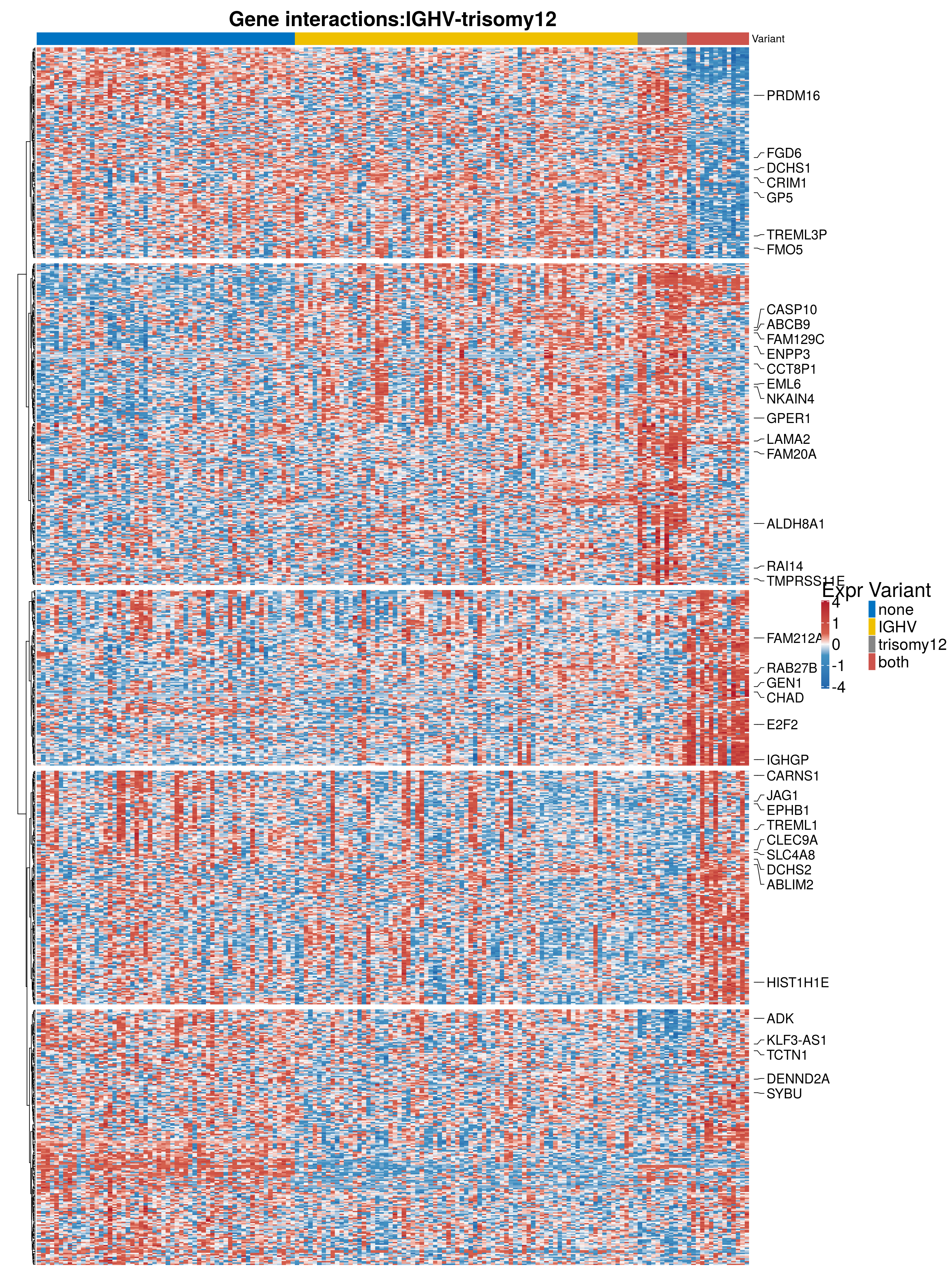
| Version | Author | Date |
|---|---|---|
| cc24f92 | aluetge | 2019-07-28 |
  #dev.off()
  #draw(h1 + ha_chrom + ha_genes)
saveRDS(p1, file = paste0(output_dir, "/figures/r_objects/epistasis/epistasis_heatmap.rds"))
IGHVTri12 <- list("sig_Genes" = sig_Genes, "geneExp" = geneExpression_new, "h1"= h1)
Genewise count distribution
#function to create stripchart plots for specific genes
gene_count <- function(gene_nam){
  geneEnsID <- rownames(ddsCLL)[which(rowData(ddsCLL)$symbol %in% gene_nam)]
  geneNum <- assay(RNAnorm)[geneEnsID,]
  mutPat <- as.data.frame(mutationStatus[colData(ddsCLL)$PatID,])
  colnames(mutPat) <- c("genotype")
  geneDat <- cbind(mutPat, geneNum)
  colnames(geneDat) <- c("genotype", "counts")

  p <- ggstripchart(geneDat, x = "genotype", y = "counts",
          color = "genotype",
          size = 3,
          palette = "jco",
          add = "mean_sd",
          title = paste(gene_nam),
          ylab = "normalized counts",
          font.x = 20, font.y = 20, font.legend = 20) +
    font("xy.text", size = 20) + font("title", size = 25, face = "bold")
 #ggsave(file=paste0("/home/almut/Dokumente/git/Transcriptome_CLL/paper/figures/epi_genes/genetic_interaction_", gene_nam, ".svg"), plot=p, width=7, height=5)
  saveRDS(p, file = paste0(output_dir, "/figures/r_objects/epistasis/de_genes/", gene_nam, ".rds"))
  p
}


#interesting genes
diff <- resTab[which(abs(resTab$stat) > 6 ),]
geneList <- diff$Symbol
geneList <- geneList[-which(geneList %in% "")]
geneList <- c(geneList, "LEF1", "TIMELESS", "CHAD", "BCL2A1", "EML6", "PPP1R14A", "EPHB6", "GEN1", "EBF1", "EBF4")


lapply(geneList, gene_count)
[[1]]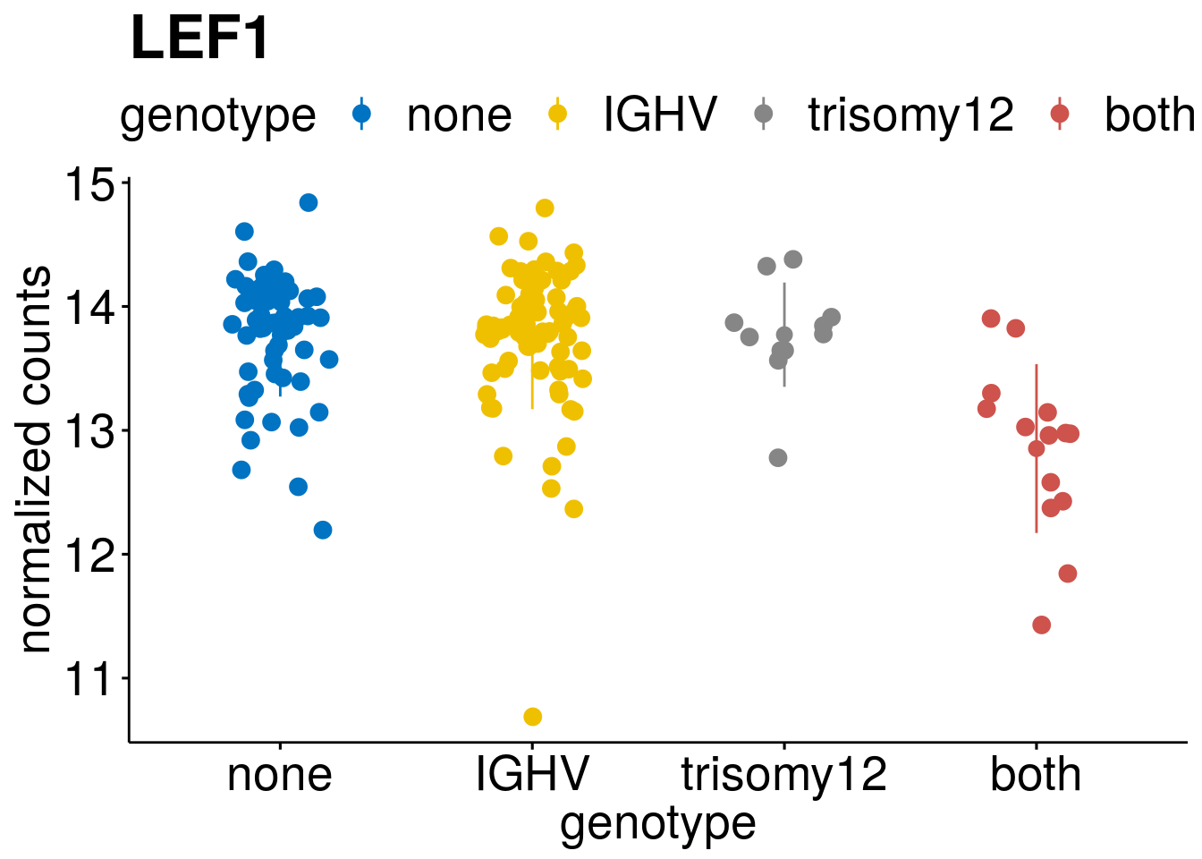
| Version | Author | Date |
|---|---|---|
| cc24f92 | aluetge | 2019-07-28 |
[[2]]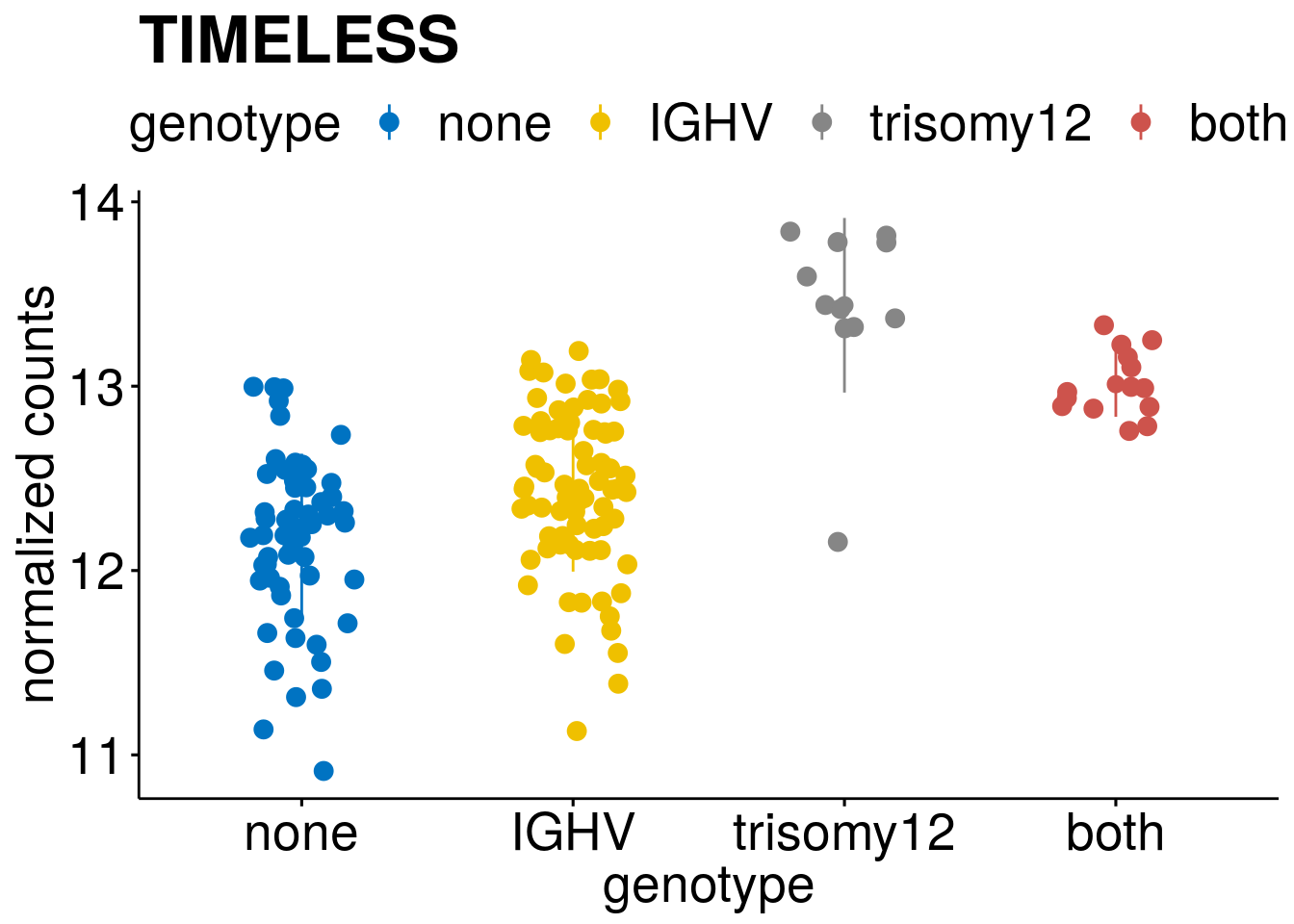
| Version | Author | Date |
|---|---|---|
| cc24f92 | aluetge | 2019-07-28 |
[[3]]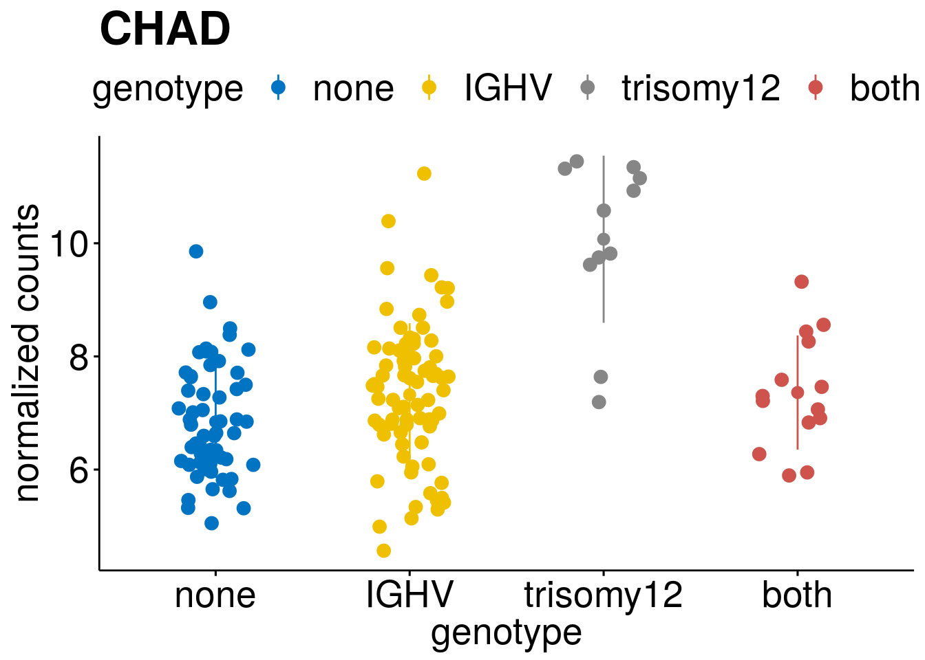
| Version | Author | Date |
|---|---|---|
| cc24f92 | aluetge | 2019-07-28 |
[[4]]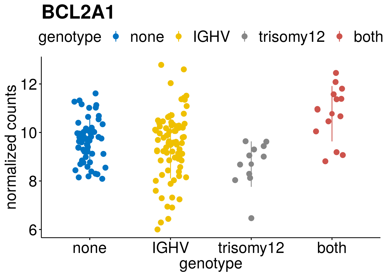
| Version | Author | Date |
|---|---|---|
| cc24f92 | aluetge | 2019-07-28 |
[[5]]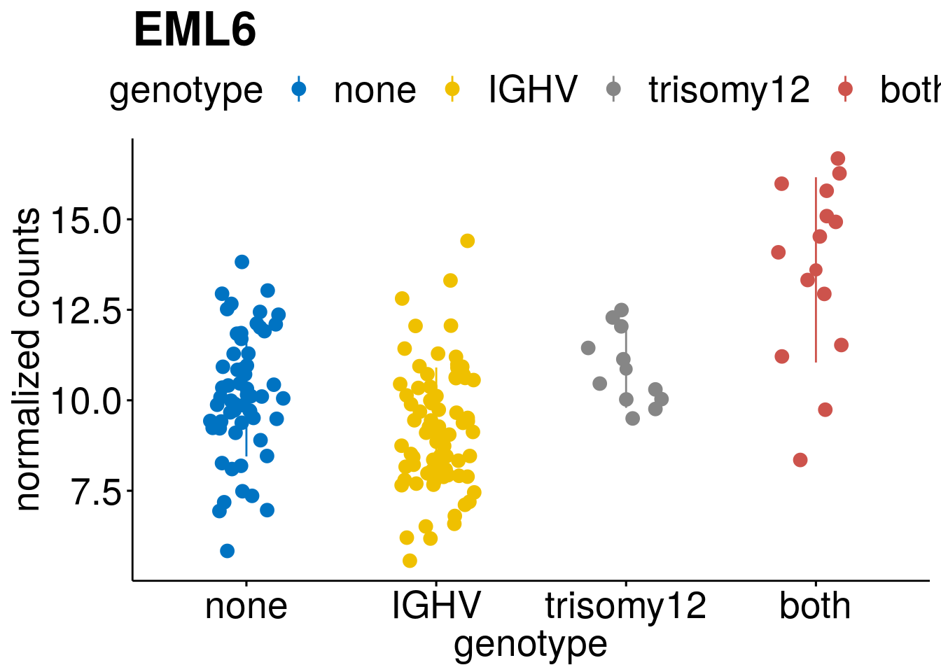
| Version | Author | Date |
|---|---|---|
| cc24f92 | aluetge | 2019-07-28 |
[[6]]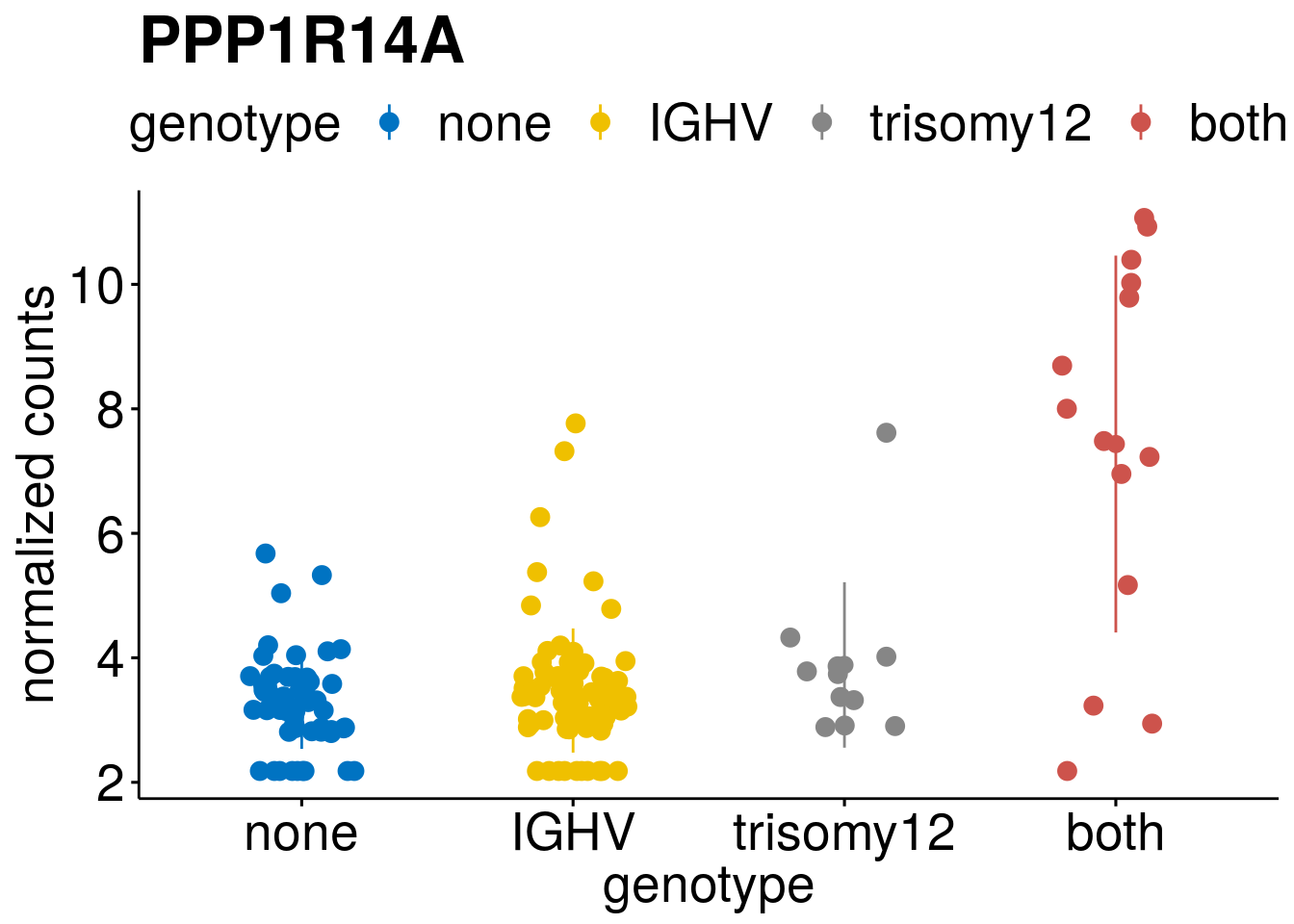
| Version | Author | Date |
|---|---|---|
| cc24f92 | aluetge | 2019-07-28 |
[[7]]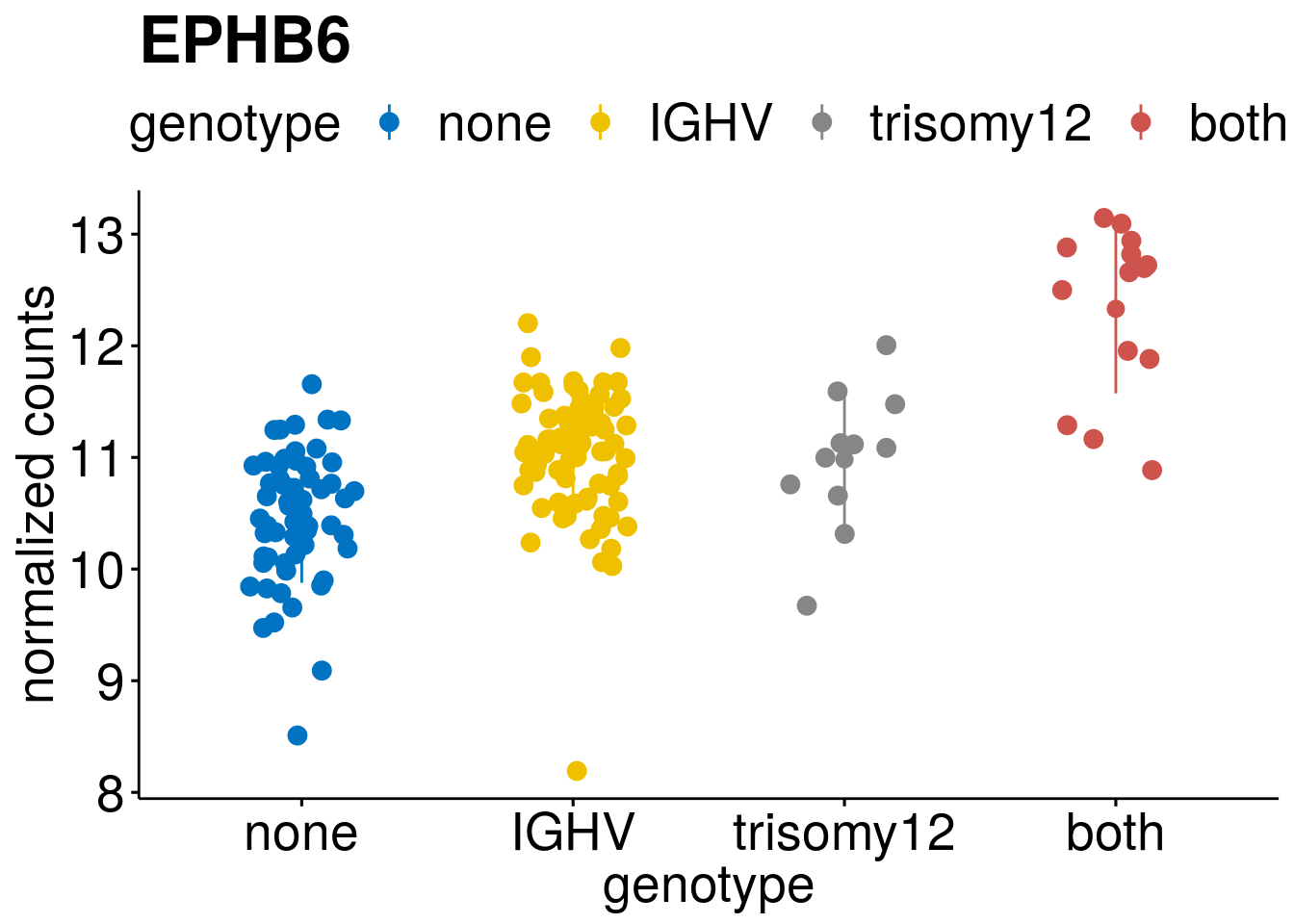
| Version | Author | Date |
|---|---|---|
| cc24f92 | aluetge | 2019-07-28 |
[[8]]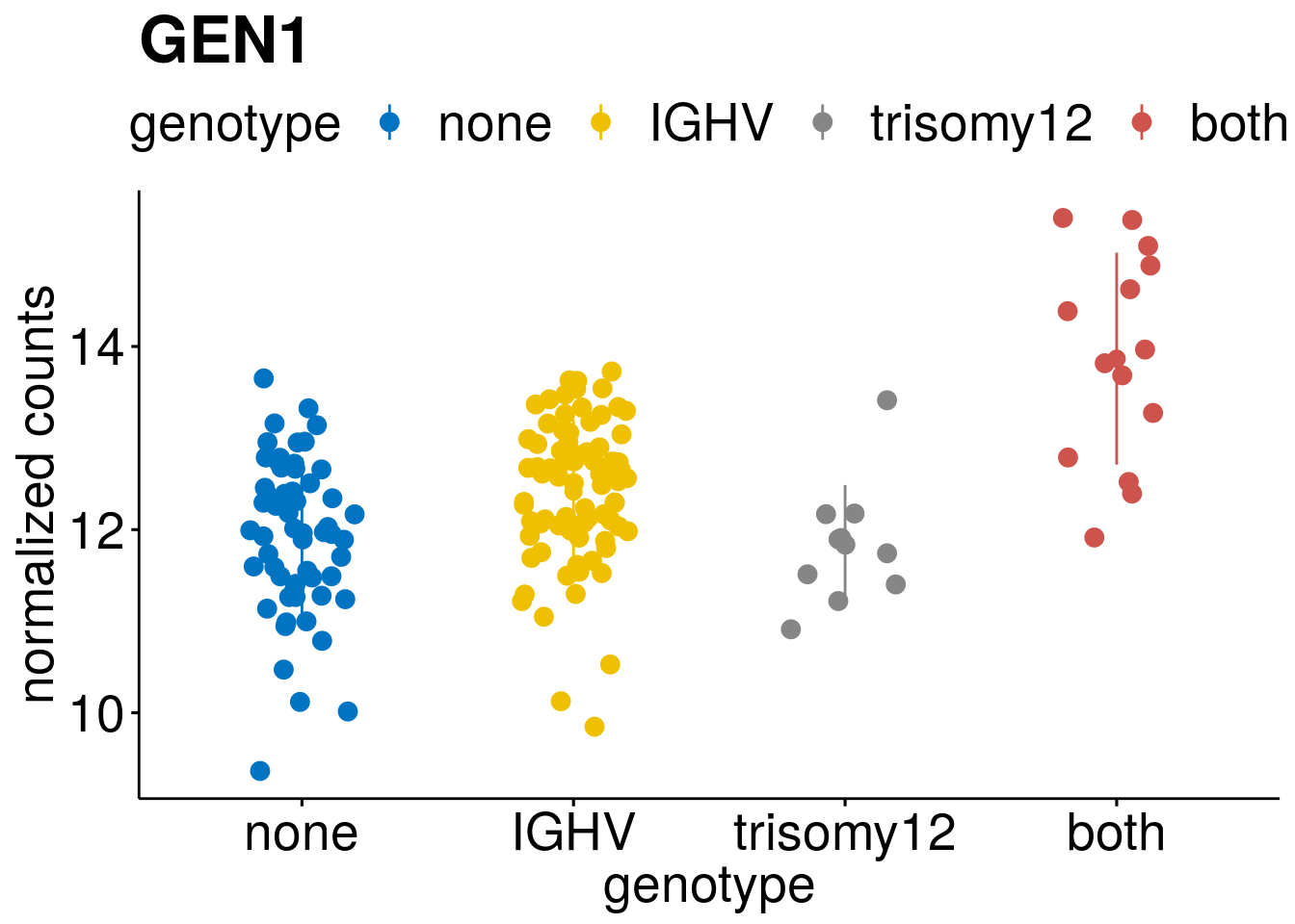
| Version | Author | Date |
|---|---|---|
| cc24f92 | aluetge | 2019-07-28 |
[[9]]
| Version | Author | Date |
|---|---|---|
| cc24f92 | aluetge | 2019-07-28 |
[[10]]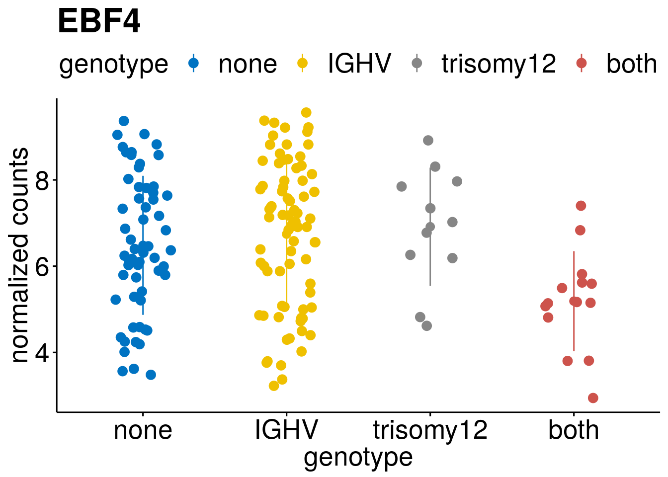
| Version | Author | Date |
|---|---|---|
| cc24f92 | aluetge | 2019-07-28 |
Clusterwise count distribution
cluster <- c("buffering_dn","sup_tri", "buffering_up" ,"buffering_up_strong", "inversion_up")

cluster_size <- lapply(c(1:5), function(clusternr){
  size <- length(row_order(IGHVTri12$h1)[[clusternr]])
  name <- cluster[clusternr]
  clust <- c(name, as.numeric(size))
}) %>% do.call(rbind,.)

cluster_size <- as.data.frame(cluster_size)
colnames(cluster_size) <- c("name", "size")
cluster_size$size <- as.numeric(as.character(cluster_size$size))
distr <- ggbarplot(cluster_size, "name", "size",
   fill = "name", color = "name",
   palette = "jco",
   ylab = "Number of genes",
   xlab = "cluster")

 #ggsave(file="/home/almut/Dokumente/masterarbeit/workinprogress/distrib_ofEpiTypes.svg", plot=distr, width=8, height=5)
distr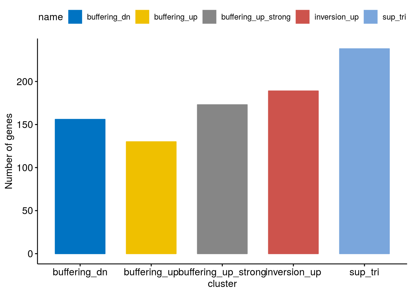
| Version | Author | Date |
|---|---|---|
| cc24f92 | aluetge | 2019-07-28 |
saveRDS(distr, file = paste0(output_dir, "/figures/r_objects/epistasis/epistasis_gene_distr.rds"))Enrichment analysis
List-based enrichment - Piano package Fisher’s exact on genes from one cluster only.
#load gene set collection

#Kegg
gsc_kegg <- loadGSC(paste0(data_dir,"/c2.cp.kegg.v6.0.symbols.gmt"), type="gmt")
#GSA on cluster defined by kmeans clustering. See cluster in heatmap...
setWiseGSA <- function(clusternr){
#get sig genes and pvalues for each cluster
geneNam <- IGHVTri12$sig_Genes[row_order(IGHVTri12$h1)[[clusternr]]]
pVal <- resSig[geneNam, "padj"]
#needs to be symbol/remove those without symbol, but ENSID only
genName <- rowData(RNAnorm[geneNam,])$symbol
gsTab <- data.frame(gene = genName, stat = pVal)
gsTab <- gsTab[-which(gsTab$gene %in% c("", NA)),]
gsaTab <- data.frame(row.names = gsTab$gene, stat = gsTab$stat)
res <- runGSA(geneLevelStats = gsaTab,
geneSetStat = "fisher",
adjMethod = "fdr", gsc=gsc_kegg,
signifMethod = 'nullDist',
#nPerm = 50000,
gsSizeLim=c(1, Inf))
Res <- arrange(GSAsummaryTable(res),desc(`Stat (non-dir.)`))
#rename results to plot
resPlot <- Res[, c(1:5)]
colnames(resPlot) <- c("pathway", "gene_number", "stat", "p", "p.adj")
#barplot
#ggplot(resPlot %>% mutate(log10Padj = -log10(p.adj)), aes(x = reorder(pathway, log10Padj), y = log10Padj, fill = gene_number)) + geom_bar(stat = "identity") + coord_flip() + ggtitle(cluster[clusternr])
enrichPlot <- resPlot[c(1:10),] %>% mutate(log10Padj = -log10(p.adj)) %>% mutate(genes = ifelse(gene_number > 5, ">5", "<=5"))
p <- ggbarplot(enrichPlot, x = "pathway", y = "log10Padj",
fill = "genes", # change fill color by mpg_level
color = "white", # Set bar border colors to white
palette = "jco", # jco journal color palett. see ?ggpar
sort.val = "asc", # Sort the value in ascending order
sort.by.groups = FALSE, # Don't sort inside each group
x.text.angle = 90, # Rotate vertically x axis texts
ylab = "-log10(padj)",
legend.title = "Pathway",
rotate = TRUE,
font.x = 20, font.y = 20, font.legend = 20, legend = "right",
title = paste0("GSEA in ", cluster[clusternr]),
ggtheme = theme_pubr()
) + font("xy.text", size = 22) + font("title", size = 20, face = "bold")
#ggsave(file=paste0("/home/almut/Dokumente/masterarbeit/results/enrichment_epistasis/GSEA_in_", clusternr, ".pdf"), plot=p, width=16, height=7)
#pdf(file= paste0("/home/almut/Dokumente/git/Transcriptome_CLL/paper/figures/GSEA_in_", clusternr, ".pdf"), width=40, height=35)
saveRDS(p, file = paste0(output_dir, "/figures/r_objects/epistasis/epistasis_", clusternr, "_enrichment.rds"))
p
# dev.off()
}
clusternr = c(1:5)
lapply(as.numeric(clusternr), setWiseGSA)Running gene set analysis:Checking arguments...done!Final gene/gene-set association: 39 genes and 70 gene sets Details: Calculating gene set statistics from 39 out of 130 gene-level statistics Removed 5227 genes from GSC due to lack of matching gene statistics Removed 116 gene sets containing no genes after gene removal Removed additionally 0 gene sets not matching the size limits Loaded additional information for 70 gene setsCalculating gene set statistics...done!
Calculating gene set significance...done!
Adjusting for multiple testing...done!Running gene set analysis:Checking arguments...done!Final gene/gene-set association: 42 genes and 71 gene sets Details: Calculating gene set statistics from 42 out of 197 gene-level statistics Removed 5224 genes from GSC due to lack of matching gene statistics Removed 115 gene sets containing no genes after gene removal Removed additionally 0 gene sets not matching the size limits Loaded additional information for 71 gene setsCalculating gene set statistics...done!
Calculating gene set significance...done!
Adjusting for multiple testing...done!Running gene set analysis:Checking arguments...done!Final gene/gene-set association: 35 genes and 51 gene sets Details: Calculating gene set statistics from 35 out of 112 gene-level statistics Removed 5231 genes from GSC due to lack of matching gene statistics Removed 135 gene sets containing no genes after gene removal Removed additionally 0 gene sets not matching the size limits Loaded additional information for 51 gene setsCalculating gene set statistics...done!
Calculating gene set significance...done!
Adjusting for multiple testing...done!Running gene set analysis:Checking arguments...done!Final gene/gene-set association: 28 genes and 63 gene sets Details: Calculating gene set statistics from 28 out of 124 gene-level statistics Removed 5238 genes from GSC due to lack of matching gene statistics Removed 123 gene sets containing no genes after gene removal Removed additionally 0 gene sets not matching the size limits Loaded additional information for 63 gene setsCalculating gene set statistics...done!
Calculating gene set significance...done!
Adjusting for multiple testing...done!Running gene set analysis:Checking arguments...done!Final gene/gene-set association: 35 genes and 66 gene sets Details: Calculating gene set statistics from 35 out of 155 gene-level statistics Removed 5231 genes from GSC due to lack of matching gene statistics Removed 120 gene sets containing no genes after gene removal Removed additionally 0 gene sets not matching the size limits Loaded additional information for 66 gene setsCalculating gene set statistics...done!
Calculating gene set significance...done!
Adjusting for multiple testing...done![[1]]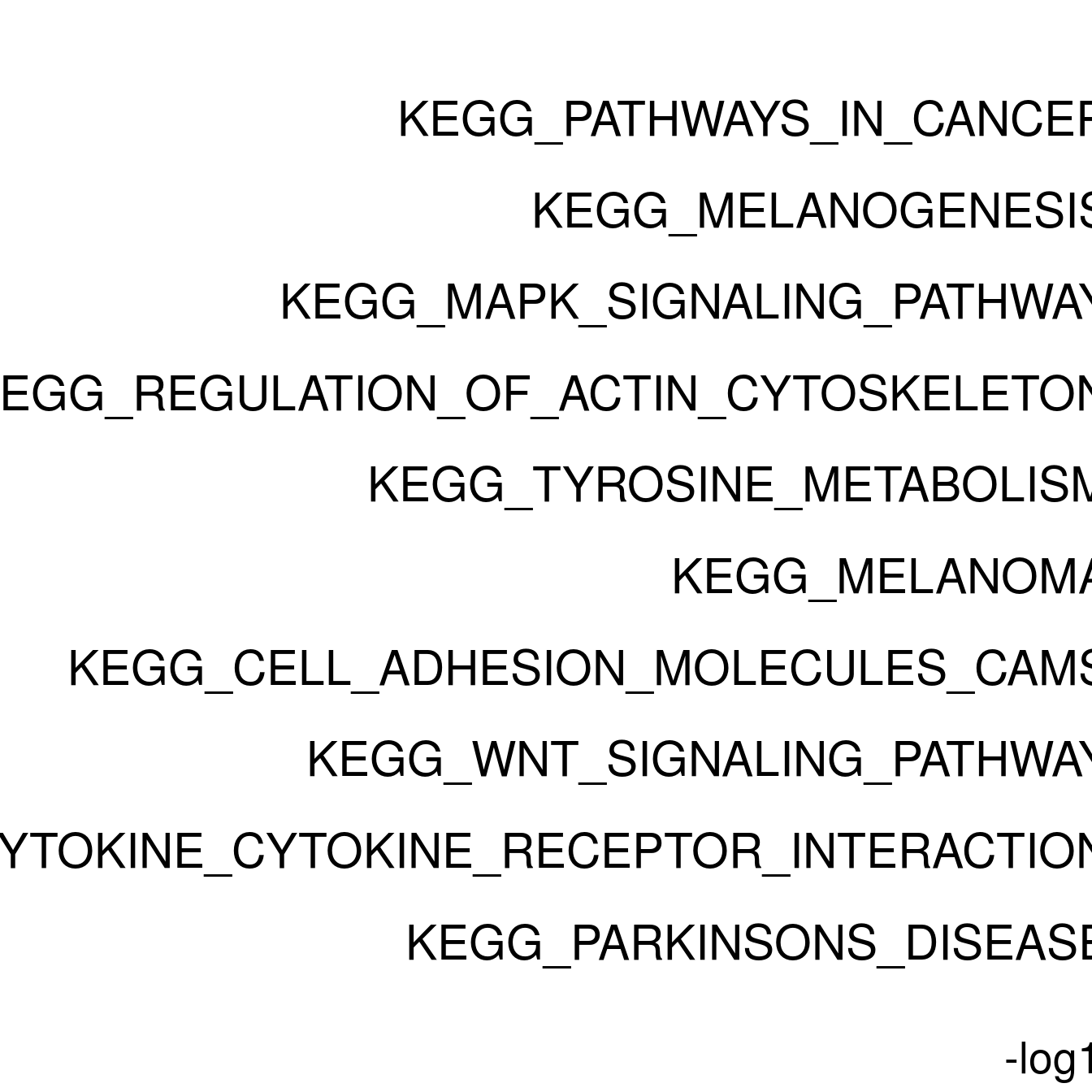
[[2]]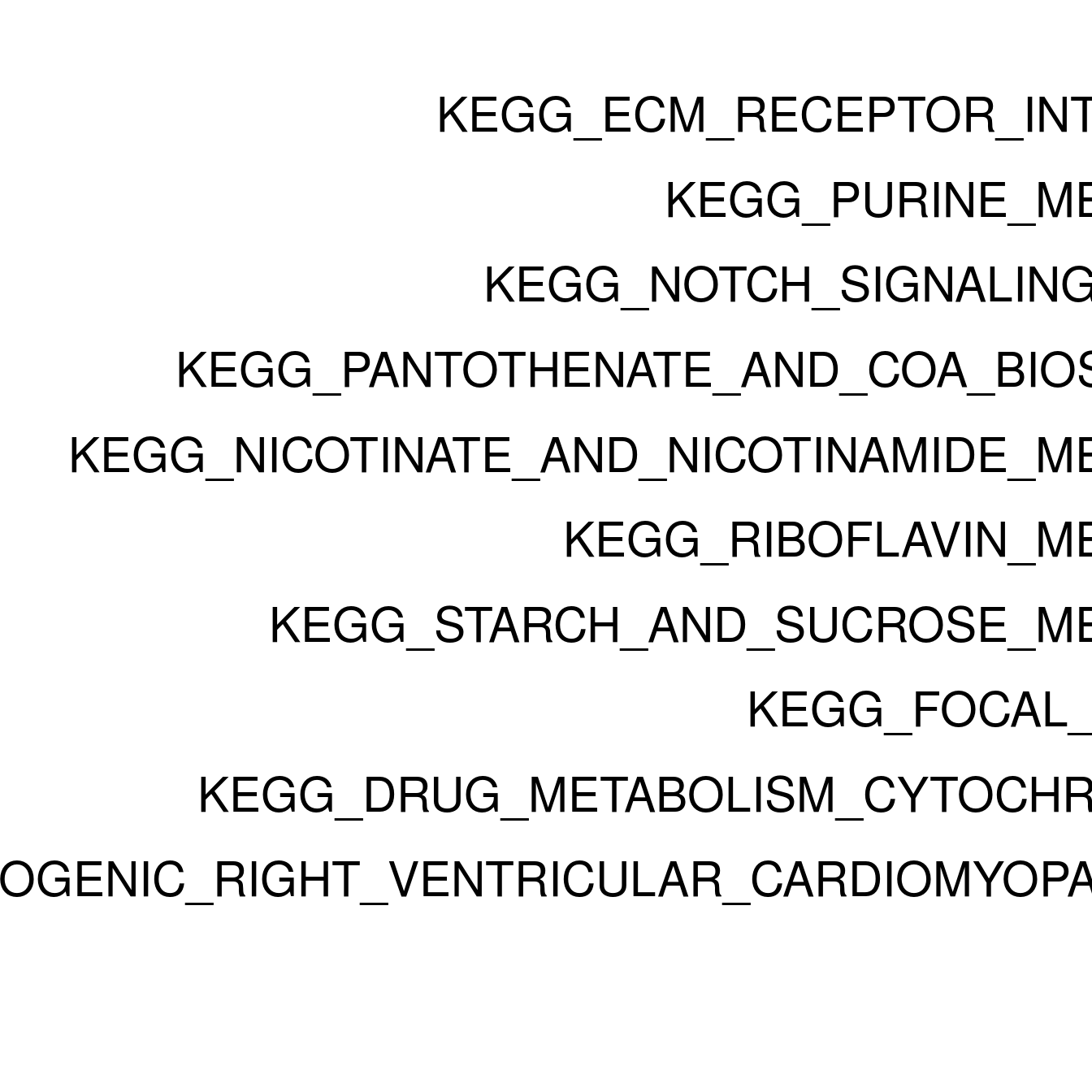
[[3]]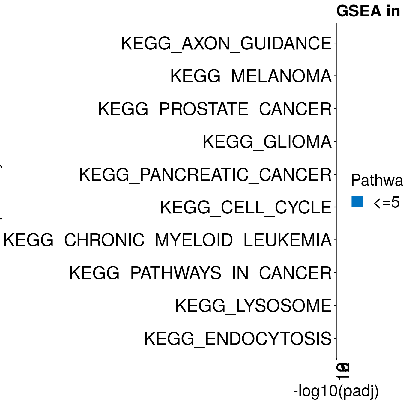
[[4]]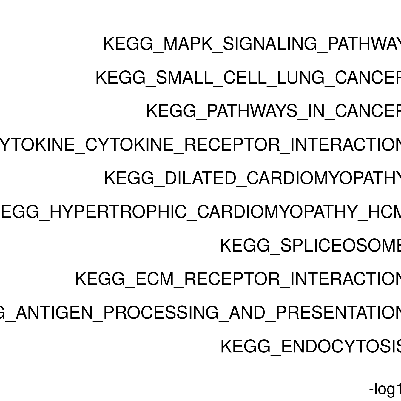
[[5]]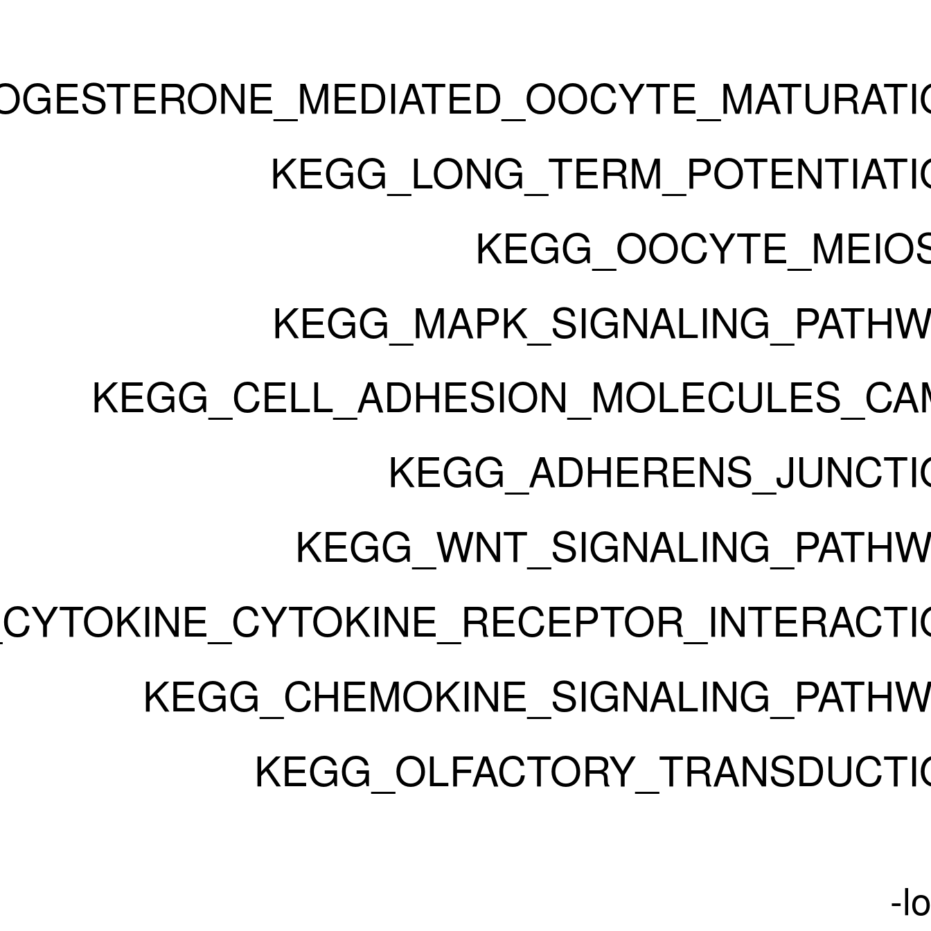
Mixed epistatsis scheme
Scheme to show different ways of mixed epistasis
#generate a dataframe
mix <- t(data.frame(buffering_up = c(-0.1, -0.5, 0.5, 5), buffering_dn = c(0.5, 0.2, -0.2, -5), suppression_1 = c(0.5, -5, -6, 0.2), suppression_2 = c(-0.2, 5, 4,-0.5), suppression_3 = c(0.5, 0.1, -6, 1), suppression_4 = c(-0.2, 0.5, 4,-0.5), inversion_up = c(-0.2, -6, -4, 5), inversion_dn = c(0.1, 5, 4, -5)))
colnames(mix) <-  c("none", "IGHV", "trisomy12", "both")

annocol <- get_palette("jco", 10)
annocolor <- list(Variant = c("none" = annocol[1], annocol[2], annocol[3], "both" = annocol[4]))
names(annocolor$Variant) <- c("none", "IGHV", "trisomy12", "both")
variants <- as.data.frame(colnames(mix))
colnames(variants) <- "Variant"
rownames(variants) <- variants$Variant

  #Column annotation
  ha_col = HeatmapAnnotation(df = variants, col = annocolor, annotation_height = unit(0.9, "cm"), annotation_legend_param = list(title_gp = gpar(fontsize = 20), labels_gp = gpar(fontsize = 15),  grid_height = unit(0.9, "cm"), grid_width = unit(0.9, "cm"), gap = unit(15, "mm")))

#heatmap
h1 <- Heatmap(mix, col = colors ,column_title = paste0("Types of mixed epistasis"), column_title_gp = gpar(fontsize = 20, fontface = "bold"), heatmap_legend_param = list(title = "Expr.", title_gp = gpar(fontsize = 20), grid_height = unit(1, "cm"), grid_width = unit(0.5, "cm"), gap = unit(10, "mm"), labels_gp = gpar(fontsize = 20), labels = c(-6,-3, 0,3, 6)) , show_row_dend = F, show_column_names =FALSE , top_annotation = ha_col, show_row_names = FALSE, show_column_dend = FALSE, cluster_columns = FALSE, cluster_rows = FALSE, split = c( rep("Buffering",2), rep("Suppression", 4), rep("Inversion", 2)), gap = unit(0.6,"cm"), row_title_gp = gpar(fontsize=19))

#pdf(file="/home/almut/Dokumente/git/Transcriptome_CLL/paper/figures/mixed_epistasis_model.pdf", width=7, height=5)
draw(h1)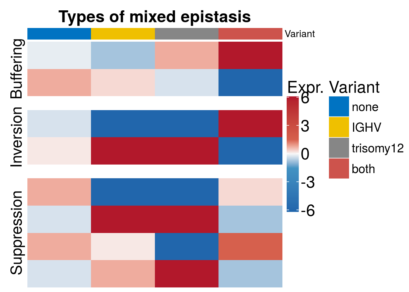
| Version | Author | Date |
|---|---|---|
| cc24f92 | aluetge | 2019-07-28 |
#dev.off()

saveRDS(h1, file = paste0(output_dir, "/figures/r_objects/epistasis/epistasis_scheme.rds"))
sessionInfo()R version 3.6.0 (2019-04-26)
Platform: x86_64-pc-linux-gnu (64-bit)
Running under: Ubuntu 16.04.6 LTS
Matrix products: default
BLAS: /usr/lib/libblas/libblas.so.3.6.0
LAPACK: /usr/lib/lapack/liblapack.so.3.6.0
locale:
[1] LC_CTYPE=de_DE.UTF-8 LC_NUMERIC=C
[3] LC_TIME=de_DE.UTF-8 LC_COLLATE=de_DE.UTF-8
[5] LC_MONETARY=de_DE.UTF-8 LC_MESSAGES=de_DE.UTF-8
[7] LC_PAPER=de_DE.UTF-8 LC_NAME=C
[9] LC_ADDRESS=C LC_TELEPHONE=C
[11] LC_MEASUREMENT=de_DE.UTF-8 LC_IDENTIFICATION=C
attached base packages:
[1] grid stats4 parallel stats graphics grDevices utils
[8] datasets methods base
other attached packages:
[1] here_0.1 ggpubr_0.2
[3] magrittr_1.5 piano_2.0.2
[5] circlize_0.4.6 ComplexHeatmap_2.0.0
[7] RColorBrewer_1.1-2 geneplotter_1.62.0
[9] annotate_1.62.0 XML_3.98-1.20
[11] AnnotationDbi_1.46.0 lattice_0.20-38
[13] dplyr_0.8.1 reshape2_1.4.3
[15] gridExtra_2.3 DESeq2_1.24.0
[17] SummarizedExperiment_1.14.0 DelayedArray_0.10.0
[19] BiocParallel_1.18.0 matrixStats_0.54.0
[21] GenomicRanges_1.36.0 GenomeInfoDb_1.20.0
[23] IRanges_2.18.1 S4Vectors_0.22.0
[25] genefilter_1.66.0 ggplot2_3.1.1
[27] Biobase_2.44.0 BiocGenerics_0.30.0
loaded via a namespace (and not attached):
[1] fgsea_1.10.0 colorspace_1.4-1 rjson_0.2.20
[4] rprojroot_1.3-2 htmlTable_1.13.1 XVector_0.24.0
[7] GlobalOptions_0.1.0 base64enc_0.1-3 fs_1.3.1
[10] clue_0.3-57 rstudioapi_0.10 DT_0.7
[13] bit64_0.9-7 splines_3.6.0 knitr_1.23
[16] jsonlite_1.6 Formula_1.2-3 workflowr_1.4.0
[19] cluster_2.1.0 png_0.1-7 shinydashboard_0.7.1
[22] shiny_1.3.2 compiler_3.6.0 backports_1.1.4
[25] assertthat_0.2.1 Matrix_1.2-17 lazyeval_0.2.2
[28] limma_3.40.2 later_0.8.0 visNetwork_2.0.7
[31] acepack_1.4.1 htmltools_0.3.6 tools_3.6.0
[34] igraph_1.2.4.1 gtable_0.3.0 glue_1.3.1
[37] GenomeInfoDbData_1.2.1 fastmatch_1.1-0 Rcpp_1.0.1
[40] slam_0.1-45 gdata_2.18.0 xfun_0.7
[43] stringr_1.4.0 mime_0.7 gtools_3.8.1
[46] zlibbioc_1.30.0 scales_1.0.0 promises_1.0.1
[49] relations_0.6-8 sets_1.0-18 yaml_2.2.0
[52] memoise_1.1.0 rpart_4.1-15 latticeExtra_0.6-28
[55] stringi_1.4.3 RSQLite_2.1.1 checkmate_1.9.3
[58] caTools_1.17.1.2 shape_1.4.4 rlang_0.3.4
[61] pkgconfig_2.0.2 bitops_1.0-6 evaluate_0.14
[64] purrr_0.3.2 labeling_0.3 htmlwidgets_1.3
[67] bit_1.1-14 tidyselect_0.2.5 ggsci_2.9
[70] plyr_1.8.4 R6_2.4.0 gplots_3.0.1.1
[73] Hmisc_4.2-0 DBI_1.0.0 pillar_1.4.1
[76] whisker_0.3-2 foreign_0.8-71 withr_2.1.2
[79] survival_2.44-1.1 RCurl_1.95-4.12 nnet_7.3-12
[82] tibble_2.1.3 crayon_1.3.4 KernSmooth_2.23-15
[85] rmarkdown_1.13 GetoptLong_0.1.7 locfit_1.5-9.1
[88] data.table_1.12.2 marray_1.62.0 blob_1.1.1
[91] git2r_0.25.2 digest_0.6.19 xtable_1.8-4
[94] httpuv_1.5.1 munsell_0.5.0 shinyjs_1.0