2_Topic_modeling
ZZ
2022-05-05
Last updated: 2022-09-21
Checks: 7 0
Knit directory: myproject/
This reproducible R Markdown analysis was created with workflowr (version 1.7.0). The Checks tab describes the reproducibility checks that were applied when the results were created. The Past versions tab lists the development history.
Great! Since the R Markdown file has been committed to the Git repository, you know the exact version of the code that produced these results.
Great job! The global environment was empty. Objects defined in the global environment can affect the analysis in your R Markdown file in unknown ways. For reproduciblity it’s best to always run the code in an empty environment.
The command set.seed(20220505) was run prior to running
the code in the R Markdown file. Setting a seed ensures that any results
that rely on randomness, e.g. subsampling or permutations, are
reproducible.
Great job! Recording the operating system, R version, and package versions is critical for reproducibility.
Nice! There were no cached chunks for this analysis, so you can be confident that you successfully produced the results during this run.
Great job! Using relative paths to the files within your workflowr project makes it easier to run your code on other machines.
Great! You are using Git for version control. Tracking code development and connecting the code version to the results is critical for reproducibility.
The results in this page were generated with repository version 460bad0. See the Past versions tab to see a history of the changes made to the R Markdown and HTML files.
Note that you need to be careful to ensure that all relevant files for
the analysis have been committed to Git prior to generating the results
(you can use wflow_publish or
wflow_git_commit). workflowr only checks the R Markdown
file, but you know if there are other scripts or data files that it
depends on. Below is the status of the Git repository when the results
were generated:
Ignored files:
    Ignored:    .DS_Store
    Ignored:    .Rhistory
    Ignored:    .Rproj.user/
    Ignored:    analysis/.DS_Store
    Ignored:    code/.DS_Store
    Ignored:    data/.DS_Store
    Ignored:    data/dictionaries/.DS_Store
    Ignored:    data/mission_statements/.DS_Store
    Ignored:    data/mission_statements/advocates/.DS_Store
    Ignored:    data/mission_statements/funders/.DS_Store
    Ignored:    data/mission_statements/journals_OA/.DS_Store
    Ignored:    data/mission_statements/journals_nonOA/.DS_Store
    Ignored:    data/mission_statements/publishers_Profit/.DS_Store
    Ignored:    data/mission_statements/publishers_nonProfit/.DS_Store
    Ignored:    data/mission_statements/repositories/.DS_Store
    Ignored:    data/mission_statements/societies/.DS_Store
    Ignored:    output/.DS_Store

Untracked files:
    Untracked:  Policy_landscape_workflowr.R
    Untracked:  code/1a_Data_preprocessing.html
    Untracked:  code/1b_Dictionaries_preparation.html
    Untracked:  code/2_Topic_modeling.html
    Untracked:  code/3_Text_similarities_Figure_2B.html
    Untracked:  code/4_Language_analysis_Figure_2C.html
    Untracked:  code/5_For_and_not_for_profit_comparison.html
    Untracked:  code/Figure_2A.html
    Untracked:  code/figure/
    Untracked:  data/mission_statements/repositories/~$nodo_Principles.doc
    Untracked:  data/mission_statements/~$RC_Vision and purpose.txt
    Untracked:  output/Figure_2A/
    Untracked:  output/Figure_2B/
    Untracked:  output/Figure_2C/
    Untracked:  output/Other_figures/
    Untracked:  output/created_datasets/

Unstaged changes:
    Deleted:    code/1a_Data_preprocessing.Rmd
    Deleted:    code/1b_Dictionaries_preparation.Rmd
    Modified:   code/README.md
Note that any generated files, e.g. HTML, png, CSS, etc., are not included in this status report because it is ok for generated content to have uncommitted changes.
These are the previous versions of the repository in which changes were
made to the R Markdown (analysis/2_Topic_modeling.Rmd) and
HTML (docs/2_Topic_modeling.html) files. If you’ve
configured a remote Git repository (see ?wflow_git_remote),
click on the hyperlinks in the table below to view the files as they
were in that past version.
| File | Version | Author | Date | Message |
|---|---|---|---|---|
| html | 796aa8e | zuzannazagrodzka | 2022-09-21 | Build site. |
| Rmd | efb1202 | zuzannazagrodzka | 2022-09-21 | Publish other files |
Topic modeling
Methods
Topic Modeling
To investigate the relationship to our research questions regarding the topics of our interest and the language choice in the stakeholders’ statements, the study employs a computational text analysis called the Structural Topic Modeling (STM) using library stm. We chose STM because it addresses the issue with the independence (like Correlated Topic Models) but also enables the discovery of topics and their prevalence based on document metadata, such as stakeholder group. The topic modeling was conducted on a sentence level and the metadata variable contained information about the stakeholders group and the document each work comes from. After generating the topics, we used the ground theory method of analysing qualitative data (Corbin and Strauss, 1990) to identify the main categories that are present in the topics.
The more detailed protocol of condensation multiple topics into a few more defined. 1. Open coding a) obtaining codes by performing STM and choosing the setting that enable the algorithm of Lee and Mimno (2014) to find the number of topics (from now on: codes). The metadata used in the modelling was the information on documents and stakeholders. The model calculates highest probability, Score, Lift and FLEX values for each word and assigns words to one or multiple topics. b) we looked at the seven words with the highest value for these four categories/values and followed a coding paradigm that enabled us to create a descriptive label for each of the code c) our paradigm contains enable us to search for words what describe or belong to missions and aims, functions, discipline and scale - Missions and aims - words are related to stakeholders’ visions, goals, statements or objectives e.g. open, free. - Functions - words associated with their roles and processes they are responsible in the research landscape e.g. publish, data, review, train - Discipline - words describing the discipline e.g. multidisciplinary, biology, ecology, evolution - Scale - words associated with the time and scale e.g. worldwide, global, long d) these will be used to create labels to describe each code
- Axial coding a) finding connections and relationships with broader categories by identifying and drawing the connections between them. It has been done by carefully going through labels and finding codes that have the same or similar descriptive labels and intuitively they are connected b) aggregating and condensing codes into broader categories based on criteria that the codes with the same or similar labels cluster together. Our aim was to end up with the smallest number of categories that we could identified.
- Selective coding a) identifying the connections between the identified categories and the rest of the codes b) removing some of the categories that we are not interested in. Many stakeholders can share topics with each other and that’s because their function in the research landscape is similar or the same. Therefore, we expect that we would not be interested in some of the codes since they would not be related to our research questions c) going through the codes again and coding accordingly to the identified main categories
There were three categories of our interests that we expected to find in the statements: 1. Related to Open Research (defined by UNESCO) 2. Related to research impact and solving global challenges 3. Related to business model or profit
Open Research and the values that it brings seems to be necessary approach to maximise impact of science and help to solve global challenges. We expect that stakeholders that care about the Open Research agenda will frequently use words such as: open, research, science, datum, access, accessibility, share, transparency
Research results and findings should be used to understand and solve challenges but also to educate people. Some stakeholders might emphasise the importance of it but not necessary seen the importance of Open Research in the process. The words that we could expect to be associated with the topic are: impact, solve, development, sustainable, education, policy, climate, change, wildlife. We also expect that words such as open, access will be absent.
In our work, we hypothesise that some organisations are run as a for profit business. Their approach could be more monetary/profit driven and therefore, they would use a business language or financial terms in their aim and mission statements. We could expect in these topics to find words such as: profit, fund, service, management, pay, financially
The stm model generated 73 topics which later were characterised and categorised following the above description. In the end we were able to identify four main topics that we called: 1. Open Research, 2. Community and Support, 3. Innovation and Solutions and 4. Publication Process. Only Open Research topic was identified as predicted beforehand.
- Open Research topic contains: Topic 1, Topic 13, Topic 58, Topic 69, Topic 43, Topic 25, Topic 32, Topic 54, Topic 52, Topic 60
- Community & Support topic contains: Topic 5, Topic 7, Topic 10, Topic 11, Topic 21, Topic 23, Topic 26, Topic 39, Topic 41, Topic 42, Topic 63, Topic 65 3.Innovation & Solution topic contains: Topic 17, Topic 24, Topic 30, Topic 14, Topic 2, Topic 34, Topic 38, Topic 4, Topic 44, Topic 48, Topic 50, Topic 51, Topic 55, Topic 61, Topic 66, Topic 71, Topic 20, Topic 57, Topic 62
- Publication process topic contains: Topic 3, Topic 12, Topic 16, Topic 22, Topic 35, Topic 49, Topic 47, Topic 53 Rest of the topics that were not able to be categorised to any of our topics were not included in our analysis and interpretation.
Topic modeling generated beta and gamma values that we later used in our analysis. Beta value is a calculated for each word and for each topic and gives information on a probability that a certain word belongs to a certain topic. Score value gives us measure how exclusive the each word is to a certain topic. For example, if a word has a low value, it means that it’s equally used in all topics. The score was calculated by a word beta value divided by a sum of beta values for this word across all topics. After merging topics into new topics that were categorised by us, we calculated mean value of the merged topics beta and score values. Later we used these values in our text similarities analysis to create Fig. 2B (3_Text_similarities, Figure_2B).
Next, we calculated the proportion of the topics appearing in all of the documents by using a mean gamma value for each sentence and new topics. The gamma value informs what is a probability that certain document (here: sentence) belongs to a certain topic. We chose one topic with the highest mean gamma value as a dominant topic for each of the sentence and later calculated the proportion of the sentences belonging to the new topics. This data set was used to create Fig. 2A (Figure_2A).
Cleaning R
rm(list=ls())Libraries
── Attaching packages ─────────────────────────────────────── tidyverse 1.3.1 ──✓ ggplot2 3.3.5 ✓ purrr 0.3.4
✓ tibble 3.1.6 ✓ dplyr 1.0.7
✓ tidyr 1.1.4 ✓ stringr 1.4.0
✓ readr 2.0.2 ✓ forcats 0.5.1── Conflicts ────────────────────────────────────────── tidyverse_conflicts() ──
x dplyr::filter() masks stats::filter()
x dplyr::lag() masks stats::lag()Package version: 3.1.0
Unicode version: 13.0
ICU version: 69.1Parallel computing: 8 of 8 threads used.See https://quanteda.io for tutorials and examples.Loading required package: NLP
Attaching package: 'NLP'The following objects are masked from 'package:quanteda':
meta, meta<-The following object is masked from 'package:ggplot2':
annotate
Attaching package: 'tm'The following object is masked from 'package:quanteda':
stopwordsLoading required package: RColorBrewer
Attaching package: 'reshape2'The following object is masked from 'package:tidyr':
smiths
Attaching package: 'igraph'The following object is masked from 'package:quanteda.textplots':
as.igraphThe following objects are masked from 'package:dplyr':
as_data_frame, groups, unionThe following objects are masked from 'package:purrr':
compose, simplifyThe following object is masked from 'package:tidyr':
crossingThe following object is masked from 'package:tibble':
as_data_frameThe following objects are masked from 'package:stats':
decompose, spectrumThe following object is masked from 'package:base':
unionstm v1.3.6 successfully loaded. See ?stm for help.
Papers, resources, and other materials at structuraltopicmodel.com
Attaching package: 'kableExtra'The following object is masked from 'package:dplyr':
group_rowsImporting data
data_words <- read.csv(file = "./output/created_datasets/cleaned_data.csv")Structural Topic Models on stakeholders
followed: https://juliasilge.com/blog/sherlock-holmes-stm/
# Creating metadata and connecting it with my data to perform topic modeling on the documents. Metadata includes: document name and stakeholder name

data_dfm <- data_words %>%
  count(sentence_doc, word, sort = TRUE) %>%
  cast_dfm(sentence_doc, word, n)

data_sparse <- data_words %>%
  count(sentence_doc, word, sort = TRUE) %>%
  cast_sparse(sentence_doc, word, n)

# Creating metadata: document name, stakeholder name
data_metadata <- data_words %>%
  select(sentence_doc, name, stakeholder) %>%
  distinct(sentence_doc, .keep_all = TRUE)

# Connecting my metadata and data_dfm for stm()
covs = data.frame(sentence_doc = data_dfm@docvars$docname, row = c(1:length(data_dfm@docvars$docname)))
covs = left_join(covs, data_metadata)
Joining, by = "sentence_doc"Topic modeling - no predetermined number of topics
data_beta <- data_words

topic_model <- stm(data_dfm, K = 0, verbose = FALSE, init.type = "Spectral", prevalence = ~ name + stakeholder, data = covs, seed = 1) # running stm() function to fit a model and generate topics
tpc = topicCorr(topic_model)
plot(tpc) # plotting topic connections, there are no clear clustering among the topics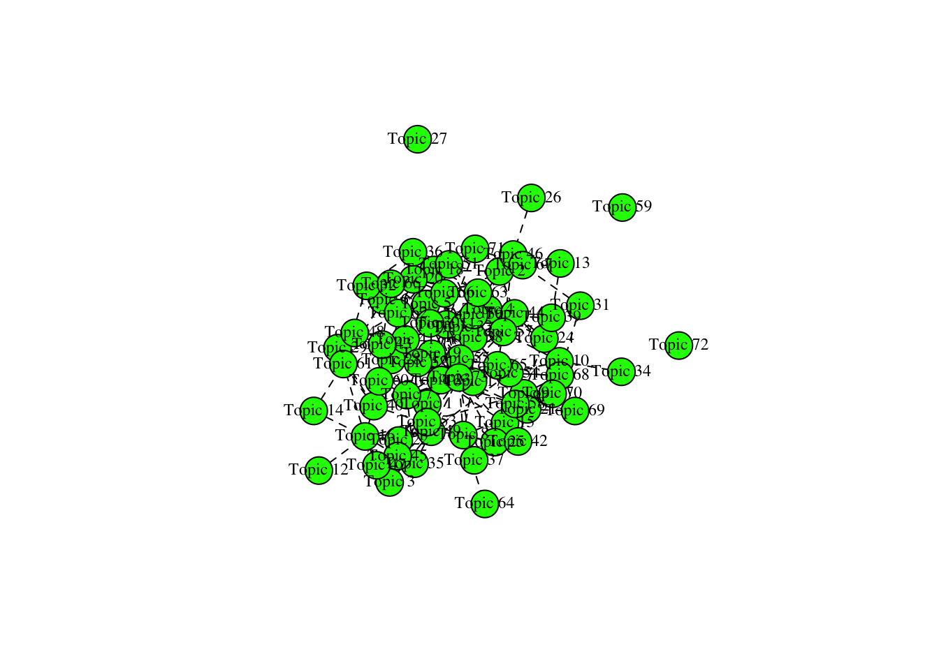
| Version | Author | Date |
|---|---|---|
| 796aa8e | zuzannazagrodzka | 2022-09-21 |
# Getting beta values from the topic modeling and adding beta value to the data_words

td_beta <- tidy(topic_model) # getting beta values
td_beta %>%
  group_by(term) %>%
  arrange(term, -beta)
# A tibble: 206,736 × 3
# Groups: term [2,832]
topic term beta
<int> <chr> <dbl>
1 27 abide 3.10e- 3
2 69 abide 1.96e- 3
3 15 abide 1.19e-169
4 56 abide 5.85e-182
5 11 abide 1.23e-199
6 9 abide 5.21e-207
7 20 abide 1.89e-209
8 73 abide 3.21e-216
9 58 abide 1.19e-239
10 21 abide 7.92e-256
# … with 206,726 more rowsMerging topics into new topics cathegories
# Topics generated by the model were coded and categorised into five defined by us topics. Below, new "topic" column was created and topics were assigned

td_beta$stm_topic <- td_beta$topic
td_beta$topic <- "NA"

# 1. Open Research topic contains: Topic 1, Topic 13, Topic 58, Topic 69, Topic 43, Topic 25, Topic 32, Topic 54, Topic 52, Topic 60
td_beta$topic[td_beta$stm_topic%in% c(1, 13, 58, 69, 43, 25, 32, 54, 52, 60)] <- 1
# 2. Community & Support topic contains: Topic 5, Topic 7, Topic 10, Topic 11, Topic 21, Topic 23, Topic 26, Topic 39, Topic 41, Topic 42, Topic 63, Topic 65
td_beta$topic[td_beta$stm_topic%in% c(5,  7,  10,  11,  21,  23,  26,  39,  41,  42,  63,  65)] <- 2
# 3.Innovation & Solution topic contains: Topic 17, Topic 24, Topic 30, Topic 14, Topic 2, Topic 34, Topic 38, Topic 4, Topic 44, Topic 48, Topic 50, Topic 51, Topic 55, Topic 61, Topic 66, Topic 71, Topic 20, Topic 57, Topic 62
td_beta$topic[td_beta$stm_topic%in% c(17,  24,  30,  14,  2,  34,  38,  4,  44,  48,  50,  51,  55,  61,  66,  71,  20,  57,  62)] <- 3
# 4. Publication process topic contains: Topic 3, Topic 12, Topic 16, Topic 22, Topic 35, Topic 49, Topic 47, Topic 53
td_beta$topic[td_beta$stm_topic%in% c(3, 12, 16, 22, 35, 49, 47, 53)] <- 4
# Rest of the topics that were not able to be categorised to any of our topics were not included in our analysis and interpretation.
td_beta$topic[td_beta$topic %in% "NA"] <- 5

td_beta$topic <- as.integer(td_beta$topic)
td_beta$term <- as.factor(td_beta$term)

# Sum of beta values for all topics for each category for each word
td_beta_sum <- td_beta %>%
  select(-stm_topic) %>%
  group_by(topic, term) %>%
  summarise(beta = sum(beta))
`summarise()` has grouped output by 'topic'. You can override using the `.groups` argument.# Mean value of beta values for all topics for each category for each word
td_beta_mean <- td_beta %>%
select(-stm_topic) %>%
group_by(topic, term) %>%
summarise(beta = mean(beta)) `summarise()` has grouped output by 'topic'. You can override using the `.groups` argument.td_beta_groups_sum <- td_beta_sum %>%
spread(topic, beta)
# Calculating score - beta value of the word in topic / total beta value for the word in all topics
td_beta_total <- td_beta %>%
group_by(term) %>%
summarise(beta_word_total = sum(beta))
td_beta_score <- td_beta %>%
left_join(td_beta_total, by = c("term" = "term"))
td_beta_score$score = td_beta_score$beta/td_beta_score$beta_word_total
head(td_beta_score)# A tibble: 6 × 6
topic term beta stm_topic beta_word_total score
<int> <fct> <dbl> <int> <dbl> <dbl>
1 1 abide 1.42e-273 1 0.00505 2.81e-271
2 3 abide 5.43e-274 2 0.00505 1.07e-271
3 4 abide 0 3 0.00505 0
4 3 abide 0 4 0.00505 0
5 2 abide 0 5 0.00505 0
6 5 abide 0 6 0.00505 0 td_beta_score <- td_beta_score %>%
select(topic, term, beta, score, stm_topic)
# Calculating mean beta and score value for new topics
# Grouping by word and then grouping by the category to calculate mean values
td_beta_mean <- td_beta_score %>%
group_by(term, topic) %>%
summarise(mean_beta = mean(beta)) %>%
mutate(merge_col = paste(term, topic, sep = "_"))`summarise()` has grouped output by 'term'. You can override using the `.groups` argument.td_score_mean <- td_beta_score %>%
group_by(term, topic) %>%
summarise(mean_score = mean(score)) %>%
mutate(merge_col = paste(term, topic, sep = "_")) %>%
ungroup() %>%
select(-term, -topic)`summarise()` has grouped output by 'term'. You can override using the `.groups` argument.# Creating a data frame with score and beta mean values
td_beta_score_mean <- td_beta_mean %>%
left_join(td_score_mean, by = c("merge_col" = "merge_col"))
# Adding a beta sum column
td_beta_sum_w <- td_beta_sum %>%
mutate(merge_col = paste(term, topic, sep = "_")) %>%
ungroup() %>%
select(- term, - topic)
td_beta_score_mean_max <- td_beta_score_mean %>%
left_join(td_beta_sum_w, by = c("merge_col" = "merge_col")) %>%
select(-merge_col) %>%
rename(sum_beta = beta)# Getting highest beta value for each of the word with the information about the Topic number
td_beta_select <- td_beta_score_mean_max
td_beta_mean_wide <- td_beta_score_mean_max %>%
select(term, topic, mean_beta) %>%
spread(topic, mean_beta) %>%
rename(mean_beta_t1 = `1`, mean_beta_t2 = `2`, mean_beta_t3 = `3`, mean_beta_t4 = `4`, mean_beta_t5 = `5`)
td_score_mean_wide <- td_beta_score_mean_max %>%
select(term, topic, mean_score) %>%
spread(topic, mean_score) %>%
rename(mean_score_t1 = `1`, mean_score_t2 = `2`, mean_score_t3 = `3`, mean_score_t4 = `4`, mean_score_t5 = `5`)
td_beta_sum_wide <- td_beta_score_mean_max %>%
select(term, topic, sum_beta) %>%
spread(topic, sum_beta) %>%
rename(sum_beta_t1 = `1`, sum_beta_t2 = `2`, sum_beta_t3 = `3`, sum_beta_t4 = `4`, sum_beta_t5 = `5`)
# Highest score value
td_score_topic <- td_beta_select %>%
select(-sum_beta, -mean_beta) %>%
group_by(term) %>%
top_n(1, mean_score) %>%
rename(highest_mean_score = mean_score)
td_score_topic %>% group_by(topic) %>% count()# A tibble: 5 × 2
# Groups: topic [5]
topic n
<int> <int>
1 1 479
2 2 439
3 3 659
4 4 502
5 5 753# Highest mean beta value
td_beta_topic <- td_beta_select %>%
select(-sum_beta, -mean_score) %>%
group_by(term) %>%
top_n(1, mean_beta) %>%
rename(highest_mean_beta = mean_beta)Creating a new dataset by merging datasets with new values
# Merging data_words with: td_beta_mean_wide, td_score_mean_wide, td_beta_sum_wide, td_score_topic
data_words$word <- as.factor(data_words$word)

to_merge <- td_beta_mean_wide %>%
  left_join(td_score_mean_wide, by= c("term" = "term")) %>%
  left_join(td_beta_sum_wide, by= c("term" = "term")) %>%
  left_join(td_score_topic, by= c("term" = "term")) %>%
  left_join(td_beta_topic, by= c("term" = "term"))

data_words_stm <- data_words %>%
  left_join(to_merge, by = c("word" = "term")) %>%
  select(-topic.y) %>%
  rename(topic = topic.x)
Saving data
# Saving the csv file
write_csv(data_words_stm, file = "./output/created_datasets/dataset_words_stm_5topics.csv")
Creating a document (sentence) level dataset
Gamma values - followed the same logic as with beta values
# Getting gamma values from topic_modeling
td_gamma <- tidy(topic_model, matrix = "gamma",
                 document_names = rownames(data_dfm))

td_gamma_prog <- td_gamma
td_gamma_prog$stm_topic <- td_gamma_prog$topic
td_gamma_prog$topic <- "NA"

td_gamma_prog$topic[td_gamma_prog$stm_topic%in% c(1, 13, 58, 69, 43, 25, 32, 54, 52, 60)] <- 1
td_gamma_prog$topic[td_gamma_prog$stm_topic%in% c(5,  7,  10,  11,  21,  23,  26,  39,  41,  42,  63,  65)] <- 2
td_gamma_prog$topic[td_gamma_prog$stm_topic%in% c(17,  24,  30,  14,  2,  34,  38,  4,  44,  48,  50,  51,  55,  61,  66,  71,  20,  57,  62)] <- 3
td_gamma_prog$topic[td_gamma_prog$stm_topic%in% c(3, 12, 16, 22, 35, 49, 47, 53)] <- 4
td_gamma_prog$topic[td_gamma_prog$topic %in% "NA"] <- 5

td_gamma_prog$topic <- as.integer(td_gamma_prog$topic)
td_gamma_prog$document <- as.factor(td_gamma_prog$document)

# Removing topic 5 as we are not interested in it
td_gamma_prog <- td_gamma_prog %>%
  select(-stm_topic) %>%
  rename(sentence_doc = document) %>%
  filter(topic != 5)

# Choosing the highest gamma value for each sentence
# Sort by the sentence and take top_n(1, gamma) to choose the topic with the biggest gamma value

td_gamma_prog_info <- td_gamma_prog %>%
  rename(topic_sentence = topic) %>%
  group_by(sentence_doc) %>%
  top_n(1, gamma) %>%
  ungroup()

# If there are any sentences with the same gamma values, I will exclude them from my analysis as not belonging to only one topic.

td_gamma_prog_info_keep <- td_gamma_prog_info %>%
  group_by(sentence_doc) %>%
  count() %>%
  filter(n == 1) %>%
  select(-n) %>%
  ungroup()

td_gamma_prog_info <- td_gamma_prog_info_keep %>%
  left_join(td_gamma_prog_info, by= c("sentence_doc" = "sentence_doc"))

# Calculating a proportion of sentences in each of the document, for that I need to add columns: document and stakeholder

# Adding info:
info_sentence_doc <- data_words %>%
  select(sentence_doc, name, stakeholder) %>%
  distinct(sentence_doc, .keep_all = TRUE)

td_gamma_prog_info <- td_gamma_prog_info %>%
  left_join(info_sentence_doc, by= c("sentence_doc"="sentence_doc"))

# Calculating proportion
# I will do so by counting name (document) to get a number of sentences in each document, then I will count a number of each topic for a document and then I will create a column with the proportion

sentence_count_gamma <- data_words %>%
  distinct(sentence_doc, .keep_all = TRUE) %>%
  group_by(name) %>%
  count() %>%
  rename(total_sent = n)

topic_count_gamma <- td_gamma_prog_info %>%
  group_by(name, topic_sentence) %>%
  count() %>%
  rename(total_topic = n)

doc_level_stm_gamma <- topic_count_gamma %>%
  left_join(sentence_count_gamma, by= c("name" = "name")) %>%
  mutate(merge_col = paste(name, topic_sentence, sep = "_"))

# There are some missing values, replacing it with 0 as not present

df_base <- info_sentence_doc %>%
  select(-sentence_doc) %>%
  distinct(name, .keep_all = TRUE) %>%
  slice(rep(1:n(), each = 4)) %>%
  group_by(name) %>%
  mutate(topic_sentence = 1:n()) %>%
  mutate(merge_col = paste(name, topic_sentence, sep = "_")) %>%
  ungroup() %>%
  select(-name, -topic_sentence)


df_doc_level_stm_gamma <- df_base %>%
  left_join(doc_level_stm_gamma, by= c("merge_col" = "merge_col")) %>%
  select(-name, -topic_sentence) %>%
  separate(merge_col, c("name","topic"), sep = "_")


df_doc_level_stm_gamma$prop <- df_doc_level_stm_gamma$total_topic/df_doc_level_stm_gamma$total_sent
df_doc_level_stm_gamma <- df_doc_level_stm_gamma %>%
    mutate_at(vars(prop), ~replace_na(., 0)) # replacing NA with 0, when a topic not present
write_excel_csv(df_doc_level_stm_gamma, "./output/created_datasets/df_doc_level_stm_gamma.csv") Additional information
Topic 1: Open Research Topic 2: Community & Support Topic 3: Innovation & Solution Topic 4: Publication process
Information about the data/topics
# Number of words belonging to new topics
no_words_topics <- data_words_stm %>%
  select(word, topic) %>%
  distinct(word, .keep_all = TRUE) %>%
  group_by(topic) %>%
  count()

no_words_topics %>%
  kbl(caption = "No of words belonging to new topics") %>%
kable_classic("hover", full_width = F)| topic | n |
|---|---|
| 1 | 479 |
| 2 | 439 |
| 3 | 659 |
| 4 | 502 |
| 5 | 753 |
# The most relevant words (15) for each topic: highest mean beta
words_high_beta_topic <- data_words_stm %>%
  select(word, topic, highest_mean_beta) %>%
  distinct(word, .keep_all = TRUE) %>%
  group_by(topic) %>%
  top_n(4) %>%
  ungroup() %>%
  arrange(topic, -highest_mean_beta)
Selecting by highest_mean_betawords_high_beta_topic %>%
kbl(caption = "Most relevant words in topics") %>%
kable_classic("hover", full_width = F)| word | topic | highest_mean_beta |
|---|---|---|
| open | 1 | 0.0565310 |
| access | 1 | 0.0302685 |
| datum | 1 | 0.0229529 |
| work | 1 | 0.0123668 |
| community | 2 | 0.0210155 |
| support | 2 | 0.0200826 |
| develop | 2 | 0.0194357 |
| knowledge | 2 | 0.0192257 |
| science | 3 | 0.0295245 |
| scientific | 3 | 0.0134324 |
| innovation | 3 | 0.0117323 |
| technology | 3 | 0.0099583 |
| publish | 4 | 0.0490068 |
| review | 4 | 0.0373344 |
| article | 4 | 0.0285216 |
| paper | 4 | 0.0279686 |
| research | 5 | 0.0589167 |
| fund | 5 | 0.0108121 |
| field | 5 | 0.0082796 |
| organisation | 5 | 0.0069668 |
Information about the stakeholders
# Advocates
advocates_info <- df_doc_level_stm_gamma %>%
  select(-total_topic, - total_sent) %>%
  filter(stakeholder == "advocates") %>%
  group_by(topic) %>%
  slice_max(order_by = prop, n = 3) %>%
  select(-stakeholder)
advocates_info
# A tibble: 12 × 3
# Groups: topic [4]
name topic prop
<chr> <chr> <dbl>
1 Jisc 1 1
2 ROpenSci 1 1
3 FAIRsharing 1 0.84
4 Reference Center for Environmental Information 2 1
5 Free our knowledge 2 0.846
6 DataCite 2 0.75
7 Research Data Canada 3 0.875
8 Gitlab 3 0.731
9 CoData 3 0.6
10 Peer Community In 4 0.75
11 Amelica 4 0.308
12 Coko 4 0.308advocates_info %>%
kbl(caption = "Advocates associated with topics") %>%
kable_classic("hover", full_width = F)| name | topic | prop |
|---|---|---|
| Jisc | 1 | 1.0000000 |
| ROpenSci | 1 | 1.0000000 |
| FAIRsharing | 1 | 0.8400000 |
| Reference Center for Environmental Information | 2 | 1.0000000 |
| Free our knowledge | 2 | 0.8461538 |
| DataCite | 2 | 0.7500000 |
| Research Data Canada | 3 | 0.8750000 |
| Gitlab | 3 | 0.7307692 |
| CoData | 3 | 0.6000000 |
| Peer Community In | 4 | 0.7500000 |
| Amelica | 4 | 0.3076923 |
| Coko | 4 | 0.3076923 |
# Funders
funders_info <- df_doc_level_stm_gamma %>%
  select(-total_topic, - total_sent) %>%
  filter(stakeholder == "funders") %>%
  group_by(topic) %>%
  slice_max(order_by = prop, n = 3) %>%
  select(-stakeholder)
funders_info
# A tibble: 14 × 3
# Groups: topic [4]
name topic prop
<chr> <chr> <dbl>
1 Sea World Research and Rescue Foundation 1 0.75
2 ERC 1 0.35
3 Max Planck Society 1 0.309
4 The French National Research Agency 2 0.857
5 Coordenacao de Aperfeicoamento de Pessoal de Nivel Superior 2 0.833
6 MOE China 2 0.762
7 CNPq 3 1
8 CONICYT 3 1
9 National Research Council Italy 3 1
10 NRC Egypt 3 1
11 Spanish National Research Council 3 1
12 Max Planck Society 4 0.0864
13 The Daimler and Benz Foundation 4 0.0833
14 Helmholtz-Gemeinschaft 4 0.08 funders_info %>%
kbl(caption = "Funders associated with topics") %>%
kable_classic("hover", full_width = F)| name | topic | prop |
|---|---|---|
| Sea World Research and Rescue Foundation | 1 | 0.7500000 |
| ERC | 1 | 0.3500000 |
| Max Planck Society | 1 | 0.3086420 |
| The French National Research Agency | 2 | 0.8571429 |
| Coordenacao de Aperfeicoamento de Pessoal de Nivel Superior | 2 | 0.8333333 |
| MOE China | 2 | 0.7619048 |
| CNPq | 3 | 1.0000000 |
| CONICYT | 3 | 1.0000000 |
| National Research Council Italy | 3 | 1.0000000 |
| NRC Egypt | 3 | 1.0000000 |
| Spanish National Research Council | 3 | 1.0000000 |
| Max Planck Society | 4 | 0.0864198 |
| The Daimler and Benz Foundation | 4 | 0.0833333 |
| Helmholtz-Gemeinschaft | 4 | 0.0800000 |
# Journals
journals_info <- df_doc_level_stm_gamma %>%
  select(-total_topic, - total_sent) %>%
  filter(stakeholder == "journals") %>%
  group_by(topic) %>%
  slice_max(order_by = prop, n = 3) %>%
  select(-stakeholder)
journals_info
# A tibble: 13 × 3
# Groups: topic [4]
name topic prop
<chr> <chr> <dbl>
1 Arctic, Antarctic, and Alpine Research 1 0.4
2 Evolutionary Applications 1 0.385
3 Remote Sensing in Ecology and Conservation 1 0.333
4 Frontiers in Ecology and Evolution 2 0.5
5 BioSciences 2 0.2
6 Global Change Biology 2 0.167
7 Global Change Biology 3 0.833
8 Ecological Applications 3 0.643
9 Philosophical Transactions of the Royal Society B 3 0.625
10 American Naturalist 4 1
11 Evolution 4 1
12 Frontiers in Ecology and the Environment 4 1
13 eLifeJournal 4 1 journals_info %>%
kbl(caption = "Journals associated with topics") %>%
kable_classic("hover", full_width = F)| name | topic | prop |
|---|---|---|
| Arctic, Antarctic, and Alpine Research | 1 | 0.4000000 |
| Evolutionary Applications | 1 | 0.3846154 |
| Remote Sensing in Ecology and Conservation | 1 | 0.3333333 |
| Frontiers in Ecology and Evolution | 2 | 0.5000000 |
| BioSciences | 2 | 0.2000000 |
| Global Change Biology | 2 | 0.1666667 |
| Global Change Biology | 3 | 0.8333333 |
| Ecological Applications | 3 | 0.6428571 |
| Philosophical Transactions of the Royal Society B | 3 | 0.6250000 |
| American Naturalist | 4 | 1.0000000 |
| Evolution | 4 | 1.0000000 |
| Frontiers in Ecology and the Environment | 4 | 1.0000000 |
| eLifeJournal | 4 | 1.0000000 |
# Publishers
publishers_info <- df_doc_level_stm_gamma %>%
  select(-total_topic, - total_sent) %>%
  filter(stakeholder == "publishers") %>%
  group_by(topic) %>%
  slice_max(order_by = prop, n = 3) %>%
  select(-stakeholder)
publishers_info
# A tibble: 12 × 3
# Groups: topic [4]
name topic prop
<chr> <chr> <dbl>
1 PeerJ 1 0.533
2 Pensoft 1 0.429
3 eLife 1 0.4
4 BioOne 2 1
5 Wiley 2 0.786
6 Elsevier 2 0.621
7 AIBS 3 1
8 Cell Press 3 0.739
9 Resilience Alliance 3 0.6
10 Pensoft 4 0.571
11 The Royal Society Publishing 4 0.5
12 The University of Chicago Press 4 0.455publishers_info %>%
kbl(caption = "Publishers associated with topics") %>%
kable_classic("hover", full_width = F)| name | topic | prop |
|---|---|---|
| PeerJ | 1 | 0.5333333 |
| Pensoft | 1 | 0.4285714 |
| eLife | 1 | 0.4000000 |
| BioOne | 2 | 1.0000000 |
| Wiley | 2 | 0.7857143 |
| Elsevier | 2 | 0.6206897 |
| AIBS | 3 | 1.0000000 |
| Cell Press | 3 | 0.7391304 |
| Resilience Alliance | 3 | 0.6000000 |
| Pensoft | 4 | 0.5714286 |
| The Royal Society Publishing | 4 | 0.5000000 |
| The University of Chicago Press | 4 | 0.4545455 |
# Repositories
repositories_info <- df_doc_level_stm_gamma %>%
  select(-total_topic, - total_sent) %>%
  filter(stakeholder == "repositories") %>%
  group_by(topic) %>%
  slice_max(order_by = prop, n = 3) %>%
  select(-stakeholder)
repositories_info
# A tibble: 12 × 3
# Groups: topic [4]
name topic prop
<chr> <chr> <dbl>
1 Marine Data Archive 1 1
2 TERN 1 1
3 Zenodo 1 0.762
4 Australian Antarctic Data Centre 2 0.625
5 World Data Center for Climate 2 0.538
6 BCO-DMO 2 0.5
7 DNA Databank of Japan 3 0.923
8 NCBI 3 0.5
9 KNB 3 0.444
10 bioRxiv 4 0.889
11 EcoEvoRxiv 4 0.4
12 Harvard Dataverse 4 0.25 repositories_info %>%
kbl(caption = "Repositories associated with topics") %>%
kable_classic("hover", full_width = F)| name | topic | prop |
|---|---|---|
| Marine Data Archive | 1 | 1.0000000 |
| TERN | 1 | 1.0000000 |
| Zenodo | 1 | 0.7619048 |
| Australian Antarctic Data Centre | 2 | 0.6250000 |
| World Data Center for Climate | 2 | 0.5384615 |
| BCO-DMO | 2 | 0.5000000 |
| DNA Databank of Japan | 3 | 0.9230769 |
| NCBI | 3 | 0.5000000 |
| KNB | 3 | 0.4444444 |
| bioRxiv | 4 | 0.8888889 |
| EcoEvoRxiv | 4 | 0.4000000 |
| Harvard Dataverse | 4 | 0.2500000 |
# Societies
societies_info <- df_doc_level_stm_gamma %>%
  select(-total_topic, - total_sent) %>%
  filter(stakeholder == "societies") %>%
  group_by(topic) %>%
  slice_max(order_by = prop, n = 3) %>%
  select(-stakeholder)
societies_info
# A tibble: 12 × 3
# Groups: topic [4]
name topic prop
<chr> <chr> <dbl>
1 Royal Society Te Aparangi 1 0.174
2 Ecological Society of Australia 1 0.0714
3 The Zoological Society of London 1 0.0357
4 European Society for Evolutionary Biology 2 1
5 American Society of Naturalists 2 0.867
6 SORTEE 2 0.667
7 Australasian Evolution Society 3 1
8 Ecological Society of America 3 1
9 The Royal Society 3 1
10 SORTEE 4 0.333
11 The Zoological Society of London 4 0.214
12 British Ecological Society 4 0.111 societies_info %>%
kbl(caption = "Societies associated with topics") %>%
kable_classic("hover", full_width = F)| name | topic | prop |
|---|---|---|
| Royal Society Te Aparangi | 1 | 0.1739130 |
| Ecological Society of Australia | 1 | 0.0714286 |
| The Zoological Society of London | 1 | 0.0357143 |
| European Society for Evolutionary Biology | 2 | 1.0000000 |
| American Society of Naturalists | 2 | 0.8666667 |
| SORTEE | 2 | 0.6666667 |
| Australasian Evolution Society | 3 | 1.0000000 |
| Ecological Society of America | 3 | 1.0000000 |
| The Royal Society | 3 | 1.0000000 |
| SORTEE | 4 | 0.3333333 |
| The Zoological Society of London | 4 | 0.2142857 |
| British Ecological Society | 4 | 0.1111111 |
Session information
sessionInfo()R version 4.0.3 (2020-10-10)
Platform: x86_64-apple-darwin17.0 (64-bit)
Running under: macOS Big Sur 10.16
Matrix products: default
BLAS: /Library/Frameworks/R.framework/Versions/4.0/Resources/lib/libRblas.dylib
LAPACK: /Library/Frameworks/R.framework/Versions/4.0/Resources/lib/libRlapack.dylib
locale:
[1] en_GB.UTF-8/en_GB.UTF-8/en_GB.UTF-8/C/en_GB.UTF-8/en_GB.UTF-8
attached base packages:
[1] stats graphics grDevices utils datasets methods base
other attached packages:
[1] kableExtra_1.3.4 stm_1.3.6
[3] ggraph_2.0.5 igraph_1.2.6
[5] reshape2_1.4.4 wordcloud_2.6
[7] RColorBrewer_1.1-2 topicmodels_0.2-12
[9] tm_0.7-8 NLP_0.2-1
[11] quanteda.dictionaries_0.3 quanteda.textplots_0.94
[13] quanteda_3.1.0 tidytext_0.3.2
[15] forcats_0.5.1 stringr_1.4.0
[17] dplyr_1.0.7 purrr_0.3.4
[19] readr_2.0.2 tidyr_1.1.4
[21] tibble_3.1.6 ggplot2_3.3.5
[23] tidyverse_1.3.1 workflowr_1.7.0
loaded via a namespace (and not attached):
[1] Rtsne_0.15 colorspace_2.0-2 ellipsis_0.3.2
[4] modeltools_0.2-23 rprojroot_2.0.2 fs_1.5.0
[7] rstudioapi_0.13 farver_2.1.0 graphlayouts_0.7.1
[10] SnowballC_0.7.0 bit64_4.0.5 ggrepel_0.9.1
[13] fansi_0.5.0 lubridate_1.7.10 xml2_1.3.2
[16] knitr_1.36 polyclip_1.10-0 jsonlite_1.7.2
[19] broom_0.7.9 dbplyr_2.1.1 ggforce_0.3.3
[22] compiler_4.0.3 httr_1.4.2 backports_1.2.1
[25] assertthat_0.2.1 Matrix_1.3-4 fastmap_1.1.0
[28] cli_3.1.0 later_1.3.0 tweenr_1.0.2
[31] htmltools_0.5.2 tools_4.0.3 rsvd_1.0.5
[34] gtable_0.3.0 glue_1.5.0 fastmatch_1.1-3
[37] Rcpp_1.0.7 slam_0.1-48 cellranger_1.1.0
[40] jquerylib_0.1.4 vctrs_0.3.8 svglite_2.0.0
[43] xfun_0.31 stopwords_2.3 ps_1.6.0
[46] rvest_1.0.1 lifecycle_1.0.1 getPass_0.2-2
[49] MASS_7.3-54 scales_1.1.1 tidygraph_1.2.0
[52] vroom_1.5.5 hms_1.1.1 promises_1.2.0.1
[55] parallel_4.0.3 yaml_2.2.1 gridExtra_2.3
[58] sass_0.4.0 stringi_1.7.5 highr_0.9
[61] tokenizers_0.2.1 geometry_0.4.5 systemfonts_1.0.2
[64] rlang_0.4.12 pkgconfig_2.0.3 evaluate_0.14
[67] lattice_0.20-45 bit_4.0.4 processx_3.5.2
[70] tidyselect_1.1.1 plyr_1.8.6 magrittr_2.0.3
[73] R6_2.5.1 generics_0.1.1 DBI_1.1.1
[76] pillar_1.6.4 haven_2.4.3 whisker_0.4
[79] withr_2.4.2 abind_1.4-5 janeaustenr_0.1.5
[82] modelr_0.1.8 crayon_1.4.2 utf8_1.2.2
[85] tzdb_0.1.2 rmarkdown_2.11 viridis_0.6.1
[88] grid_4.0.3 readxl_1.3.1 data.table_1.14.2
[91] callr_3.7.0 git2r_0.29.0 webshot_0.5.2
[94] reprex_2.0.1 digest_0.6.28 httpuv_1.6.3
[97] RcppParallel_5.1.4 stats4_4.0.3 munsell_0.5.0
[100] viridisLite_0.4.0 bslib_0.3.0 magic_1.6-0