Text_similarities
ZZ
2022-05-05
Last updated: 2022-09-21
Checks: 7 0
Knit directory: myproject/
This reproducible R Markdown analysis was created with workflowr (version 1.7.0). The Checks tab describes the reproducibility checks that were applied when the results were created. The Past versions tab lists the development history.
Great! Since the R Markdown file has been committed to the Git repository, you know the exact version of the code that produced these results.
Great job! The global environment was empty. Objects defined in the global environment can affect the analysis in your R Markdown file in unknown ways. For reproduciblity it’s best to always run the code in an empty environment.
The command set.seed(20220505) was run prior to running
the code in the R Markdown file. Setting a seed ensures that any results
that rely on randomness, e.g. subsampling or permutations, are
reproducible.
Great job! Recording the operating system, R version, and package versions is critical for reproducibility.
Nice! There were no cached chunks for this analysis, so you can be confident that you successfully produced the results during this run.
Great job! Using relative paths to the files within your workflowr project makes it easier to run your code on other machines.
Great! You are using Git for version control. Tracking code development and connecting the code version to the results is critical for reproducibility.
The results in this page were generated with repository version 460bad0. See the Past versions tab to see a history of the changes made to the R Markdown and HTML files.
Note that you need to be careful to ensure that all relevant files for
the analysis have been committed to Git prior to generating the results
(you can use wflow_publish or
wflow_git_commit). workflowr only checks the R Markdown
file, but you know if there are other scripts or data files that it
depends on. Below is the status of the Git repository when the results
were generated:
Ignored files:
    Ignored:    .DS_Store
    Ignored:    .Rhistory
    Ignored:    .Rproj.user/
    Ignored:    analysis/.DS_Store
    Ignored:    code/.DS_Store
    Ignored:    data/.DS_Store
    Ignored:    data/dictionaries/.DS_Store
    Ignored:    data/mission_statements/.DS_Store
    Ignored:    data/mission_statements/advocates/.DS_Store
    Ignored:    data/mission_statements/funders/.DS_Store
    Ignored:    data/mission_statements/journals_OA/.DS_Store
    Ignored:    data/mission_statements/journals_nonOA/.DS_Store
    Ignored:    data/mission_statements/publishers_Profit/.DS_Store
    Ignored:    data/mission_statements/publishers_nonProfit/.DS_Store
    Ignored:    data/mission_statements/repositories/.DS_Store
    Ignored:    data/mission_statements/societies/.DS_Store
    Ignored:    output/.DS_Store

Untracked files:
    Untracked:  Policy_landscape_workflowr.R
    Untracked:  code/1a_Data_preprocessing.html
    Untracked:  code/1b_Dictionaries_preparation.html
    Untracked:  code/2_Topic_modeling.html
    Untracked:  code/3_Text_similarities_Figure_2B.html
    Untracked:  code/4_Language_analysis_Figure_2C.html
    Untracked:  code/5_For_and_not_for_profit_comparison.html
    Untracked:  code/Figure_2A.html
    Untracked:  code/figure/
    Untracked:  data/mission_statements/repositories/~$nodo_Principles.doc
    Untracked:  data/mission_statements/~$RC_Vision and purpose.txt
    Untracked:  output/Figure_2A/
    Untracked:  output/Figure_2B/
    Untracked:  output/Figure_2C/
    Untracked:  output/Other_figures/
    Untracked:  output/created_datasets/

Unstaged changes:
    Deleted:    code/1a_Data_preprocessing.Rmd
    Deleted:    code/1b_Dictionaries_preparation.Rmd
    Modified:   code/README.md
Note that any generated files, e.g. HTML, png, CSS, etc., are not included in this status report because it is ok for generated content to have uncommitted changes.
These are the previous versions of the repository in which changes were
made to the R Markdown
(analysis/3_Text_similarities_Figure_2B.Rmd) and HTML
(docs/3_Text_similarities_Figure_2B.html) files. If you’ve
configured a remote Git repository (see ?wflow_git_remote),
click on the hyperlinks in the table below to view the files as they
were in that past version.
| File | Version | Author | Date | Message |
|---|---|---|---|---|
| html | 796aa8e | zuzannazagrodzka | 2022-09-21 | Build site. |
| Rmd | efb1202 | zuzannazagrodzka | 2022-09-21 | Publish other files |
Source of the functions: https://www.markhw.com/blog/word-similarity-graphs
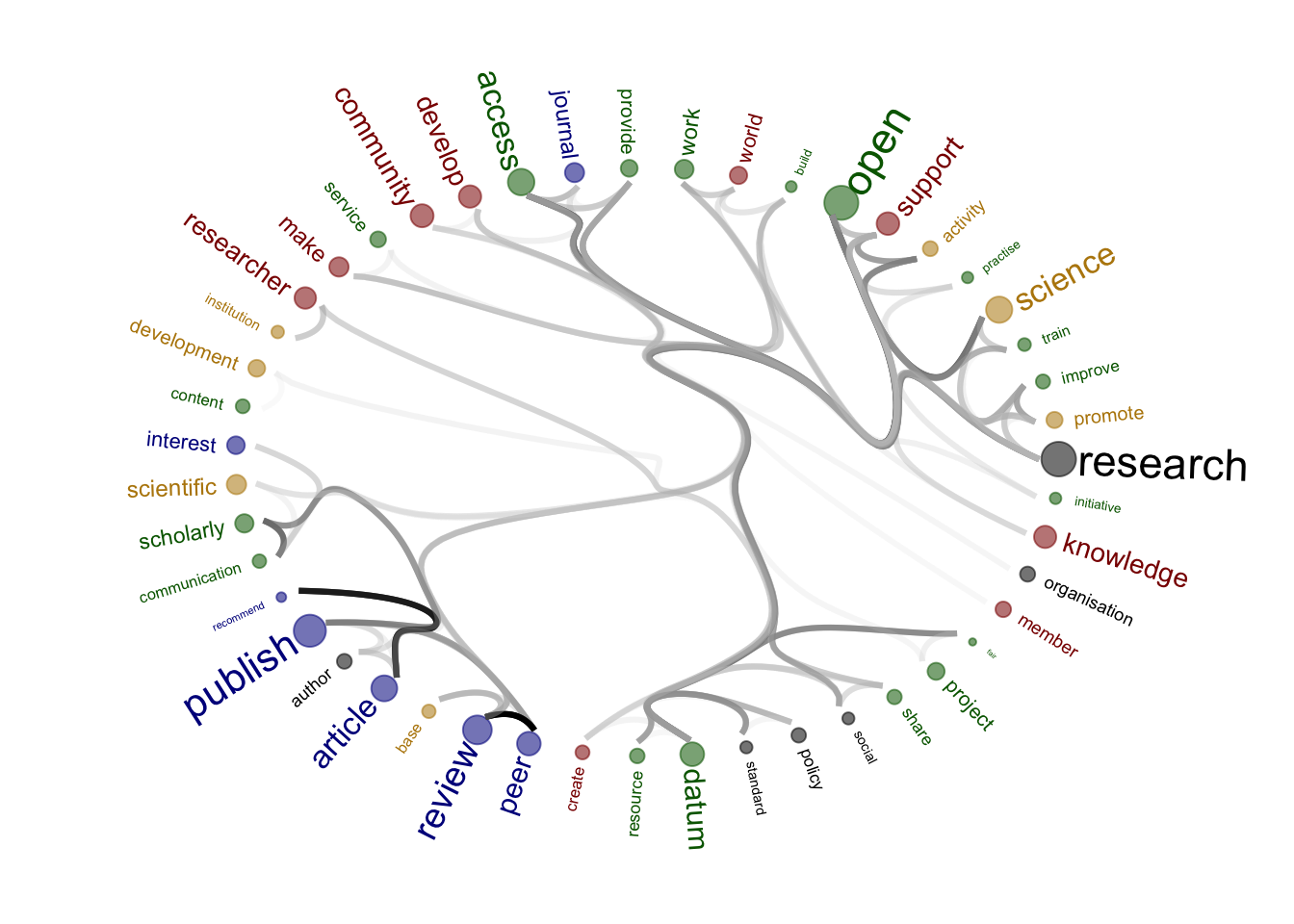
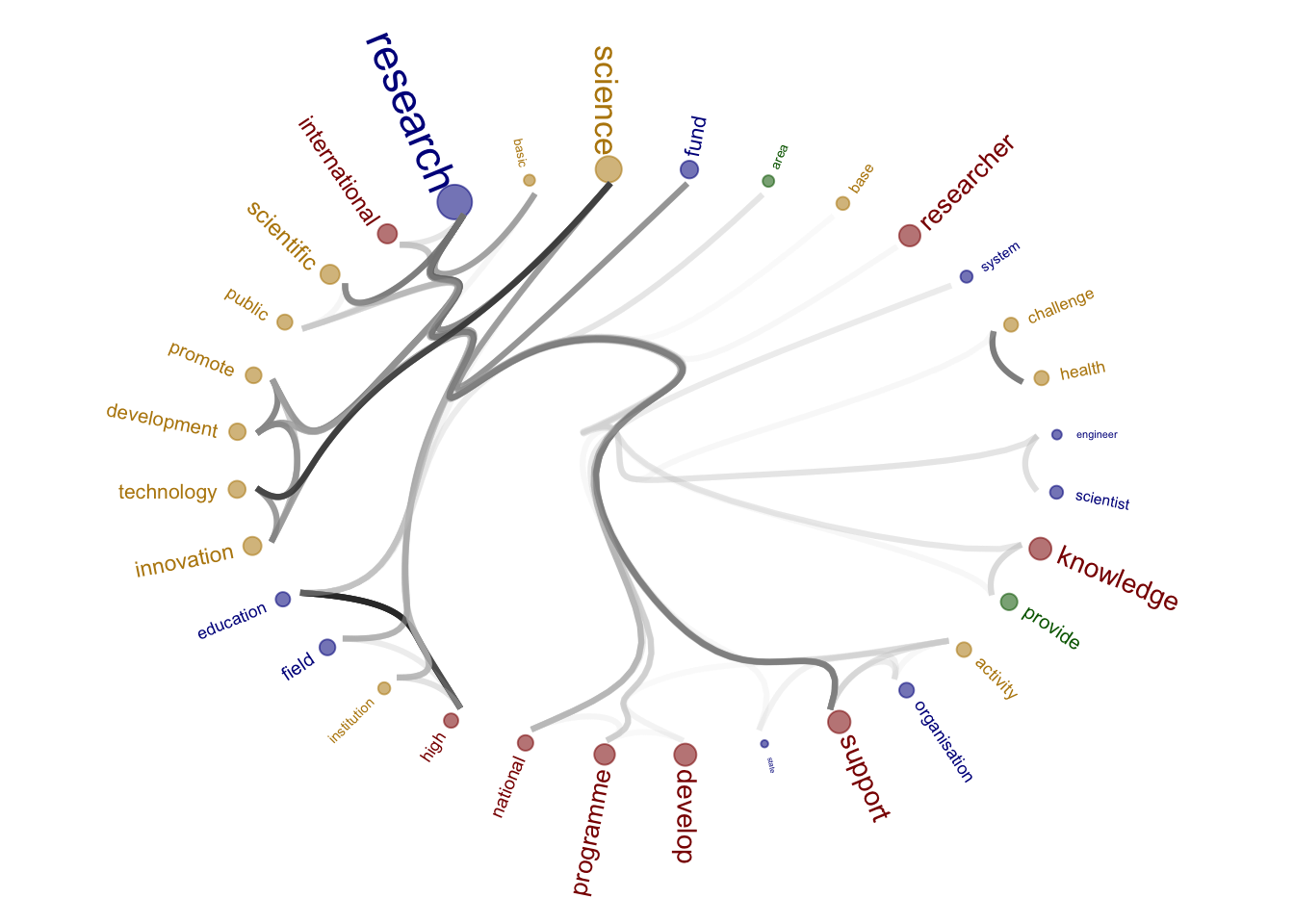
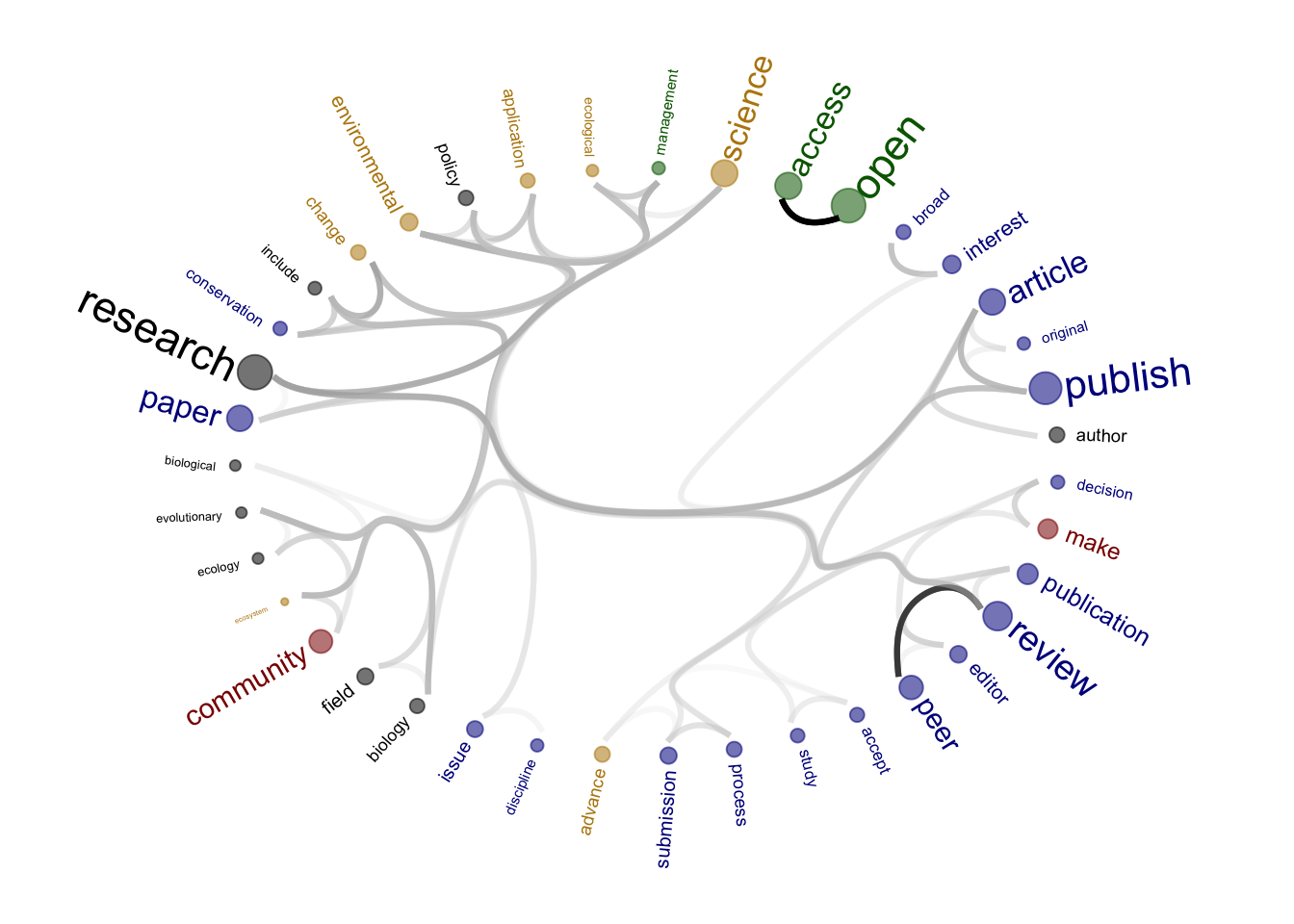
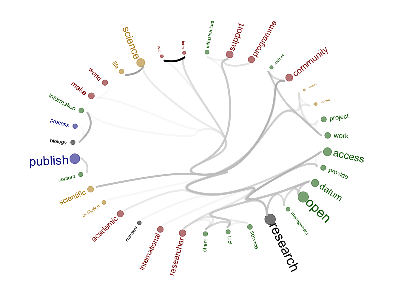
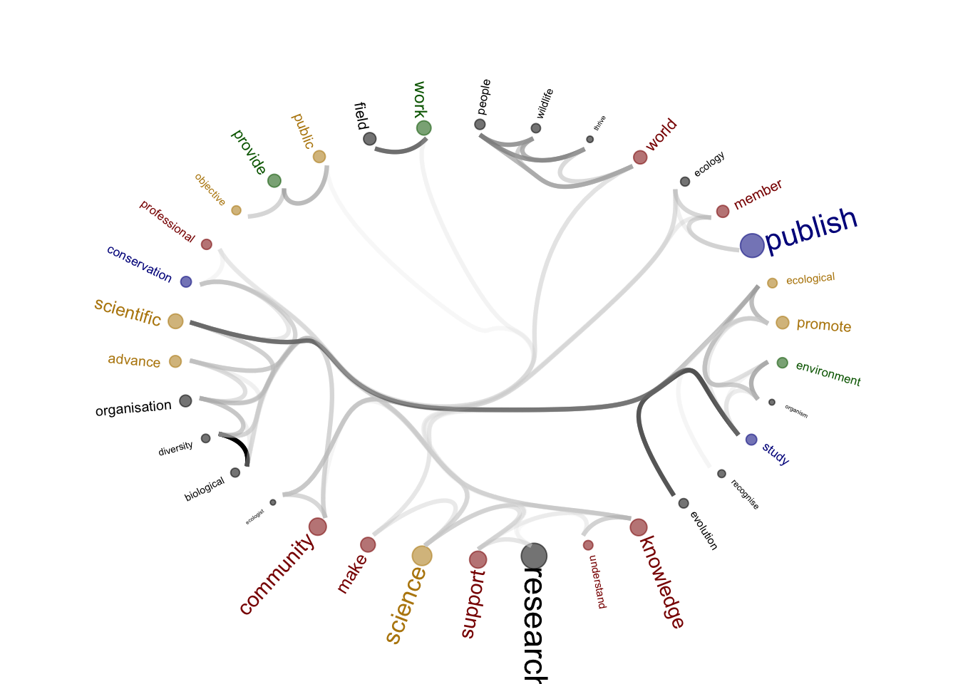
We combined two methods to be able visually explore topics and words’ connections in the aims and missions documents. We used the word similarity method (https://www.markhw.com/blog/word-similarity-graphs) to calculate similarities between words and later to be able to plot them with topic modeling score values (package stm)
The three primary steps were followed: 1. Calculating the similarities between words (Cosine matrix).
Formatting these similarity scores into a symmetric matrix, where the diagonal contains 0s and the off-diagonal cells are similarities between words.
Clustering nodes using a community detection algorithm (here: Walktrap algorithm) and plotting the data into circular hierarchical dendrograms for each of the stakeholder group separately (Figure 2B).
Libraries
# remotes::install_github('talgalili/dendextend')
library(dendextend)
---------------------
Welcome to dendextend version 1.15.3
Type citation('dendextend') for how to cite the package.

Type browseVignettes(package = 'dendextend') for the package vignette.
The github page is: https://github.com/talgalili/dendextend/

Suggestions and bug-reports can be submitted at: https://github.com/talgalili/dendextend/issues
You may ask questions at stackoverflow, use the r and dendextend tags:
     https://stackoverflow.com/questions/tagged/dendextend

    To suppress this message use:  suppressPackageStartupMessages(library(dendextend))
---------------------
Attaching package: 'dendextend'The following object is masked from 'package:stats':
cutreelibrary(igraph)
Attaching package: 'igraph'The following objects are masked from 'package:stats':
decompose, spectrumThe following object is masked from 'package:base':
unionlibrary(ggraph)Loading required package: ggplot2library(reshape2)
library(dplyr)
Attaching package: 'dplyr'The following objects are masked from 'package:igraph':
as_data_frame, groups, unionThe following objects are masked from 'package:stats':
filter, lagThe following objects are masked from 'package:base':
intersect, setdiff, setequal, unionlibrary(tidyverse)── Attaching packages ─────────────────────────────────────── tidyverse 1.3.1 ──✓ tibble 3.1.6 ✓ purrr 0.3.4
✓ tidyr 1.1.4 ✓ stringr 1.4.0
✓ readr 2.0.2 ✓ forcats 0.5.1── Conflicts ────────────────────────────────────────── tidyverse_conflicts() ──
x tibble::as_data_frame() masks dplyr::as_data_frame(), igraph::as_data_frame()
x purrr::compose() masks igraph::compose()
x tidyr::crossing() masks igraph::crossing()
x dplyr::filter() masks stats::filter()
x dplyr::groups() masks igraph::groups()
x dplyr::lag() masks stats::lag()
x purrr::simplify() masks igraph::simplify()library(tidytext)Below chunk contain functions which were used to create words similarities matrix. Source of the code:
https://www.markhw.com/blog/word-similarity-graphs
# Cosine matrix
cosine_matrix <- function(tokenized_data, lower = 0, upper = 1, filt = 0) {

  if (!all(c("word", "id") %in% names(tokenized_data))) {
    stop("tokenized_data must contain variables named word and id")
  }

  if (lower < 0 | lower > 1 | upper < 0 | upper > 1 | filt < 0 | filt > 1) {
    stop("lower, upper, and filt must be 0 <= x <= 1")
  }
  docs <- length(unique(tokenized_data$id))

  out <- tokenized_data %>%
    count(id, word) %>%
    group_by(word) %>%
    mutate(n_docs = n()) %>%
    ungroup() %>%
    filter(n_docs <= (docs * upper) & n_docs > (docs * lower)) %>%
    select(-n_docs) %>%
    mutate(n = 1) %>%
    spread(word, n, fill = 0) %>%
    select(-id) %>%
    as.matrix() %>%
    lsa::cosine()

  filt <- quantile(out[lower.tri(out)], filt)
  out[out < filt] <- diag(out) <- 0
  out <- out[rowSums(out) != 0, colSums(out) != 0]

  return(out)
}


# Walktrap_topics

walktrap_topics <- function(g, ...) {
  wt <- igraph::cluster_walktrap(g, ...)

  membership <- igraph::cluster_walktrap(g, ...) %>%
      igraph::membership() %>%
      as.matrix() %>%
      as.data.frame() %>%
      rownames_to_column("word") %>%
      arrange(V1) %>%
      rename(group = V1)

  dendrogram <- stats::as.dendrogram(wt)

  return(list(membership = membership, dendrogram = dendrogram))
}
Importing data
corpus_df <- read.csv("./output/created_datasets/dataset_words_stm_5topics.csv")Running above functions for each stakeholder seperately
corpus_df <- read.csv("./output/created_datasets/dataset_words_stm_5topics.csv")
stake_names <- unique(corpus_df$stakeholder)
count <- 1
figure_list <- vector()

for (stake in stake_names) {
  n <- count # number of the stakeholder in the list
  stakeholder_name <- stake_names[n] # stakeholder's name

  # selecting data with the right name of the stakeholder
  dat <- corpus_df %>%
  select(stakeholder, sentence_doc, word) %>%
  rename(id = sentence_doc) %>%
  filter(stakeholder %in% stakeholder_name) %>%
  select(-stakeholder)
  #####################

  # Calculating similarity matrix
  cos_mat <- cosine_matrix(dat, lower = 0.050, upper = 1, filt = 0.9)

  # Getting words used in the network
  word_list_net <- rownames(cos_mat)
  grep("workflow", word_list_net)

  print(dim(cos_mat))

  # Creating a graph
  g <- graph_from_adjacency_matrix(cos_mat, mode = "undirected", weighted = TRUE)
  topics = walktrap_topics(g)
  print(stakeholder_name)
  plot(topics$dendrogram)

  subtrees <- partition_leaves(topics$dendrogram)
  leaves <- subtrees[[1]]


  pathRoutes <- function(leaf) {
    which(sapply(subtrees, function(x) leaf %in% x))
  }

  paths <- lapply(leaves, pathRoutes)

  edges = NULL
  for(a in 1:length(paths)){
    # print(a)
    for(b in c(1:(length(paths[[a]])-1))){
     if(b == (length(paths[[a]])-1)){
        tmp_df = data.frame(
         from = paths[[a]][b],
         to = leaves[a]
       )
     } else {
        tmp_df = data.frame(
          from = paths[[a]][b],
          to = paths[[a]][b+1]
       )
     }
     edges = rbind(edges, tmp_df)
   }
  }


  connect = melt(cos_mat) # library reshape required
  colnames(connect) = c("from", "to", "value")
  connect = subset(connect, value != 0)

  # create a vertices data.frame. One line per object of our hierarchy
  vertices  <-  data.frame(
    name = unique(c(as.character(edges$from), as.character(edges$to)))
  )
  # Let's add a column with the group of each name. It will be useful later to color points
  vertices$group  <-  edges$from[ match( vertices$name, edges$to ) ]


  #Let's add information concerning the label we are going to add: angle, horizontal adjustement and potential flip
  #calculate the ANGLE of the labels
  #vertices$id <- NA
  #myleaves <- which(is.na( match(vertices$name, edges$from) ))
  #nleaves <- length(myleaves)
  #vertices$id[ myleaves ] <- seq(1:nleaves)
  #vertices$angle <- 90 - 360 * vertices$id / nleaves

  # calculate the alignment of labels: right or left
  # If I am on the left part of the plot, my labels have currently an angle < -90
  #vertices$hjust <- ifelse( vertices$angle < -90, 1, 0)

  # flip angle BY to make them readable
  #vertices$angle <- ifelse(vertices$angle < -90, vertices$angle+180, vertices$angle)

  # replacing "group" value with the topic numer from the STM

  # Colour words by topic modelling topics (STM)
  # I have to change the group numbers in topics

  stm_top <- corpus_df %>%
    select(stakeholder, word, topic = topic) %>%
    filter(stakeholder %in% stakeholder_name) %>%
    select(-stakeholder)


  stm_top$topic <- as.factor(stm_top$topic)
  stm_top <- unique(stm_top)


  # Removing group column and creating a new one based on the stm info
  vertices <- vertices

  vertices <- vertices %>%
    left_join(stm_top, by = c("name" = "word")) %>%
    select(-group) %>%
    rename(group = topic)

  # Adding a beta value so I can use it in the graph
  stm_beta <- corpus_df %>%
    select(stakeholder, word, beta = highest_mean_beta) %>%
    filter(stakeholder %in% stakeholder_name) %>%
    select(-stakeholder)


  stm_beta <- unique(stm_beta)
  dim(stm_beta)

  vertices <- vertices %>%
   left_join(stm_beta, by = c("name" = "word"))


  vertices$beta_size = vertices$beta

  ##############################################################

  # Create a graph object
  mygraph <- igraph::graph_from_data_frame(edges, vertices=vertices)

  # The connection object must refer to the ids of the leaves:
  from  <-  match( connect$from, vertices$name)
  to  <-  match( connect$to, vertices$name)

  # Basic usual argument
  tmp_plt = ggraph(mygraph, layout = 'dendrogram', circular = T) +
    geom_node_point(aes(filter = leaf, x = x*1.05, y=y*1.05, alpha=0.2), size =0, colour = "white") +
    #colour=group, size=value
          scale_colour_manual(values= c("dark green", "dark red", "darkgoldenrod", "dark blue", "black"), na.value = "black") +
    geom_conn_bundle(data = get_con(from = from, to = to, col = connect$value), tension = 0.9, aes(colour = col, alpha = col+0.5), width = 1.1) +
    scale_edge_color_continuous(low="white", high="black") +
    # geom_node_text(aes(x = x*1.1, y=y*1.1, filter = leaf, label=name, angle = angle, hjust=hjust), size=5, alpha=1) +
    geom_node_text(aes(x = x*1.1, y=y*1.1, filter = leaf, label=name, colour = group, angle = 0, hjust = 0.5, size = beta_size),  alpha=1) +

     theme_void() +
    theme(
      legend.position="none",
      plot.margin=unit(c(0,0,0,0),"cm"),
    ) +
    expand_limits(x = c(-1.5, 1.5), y = c(-1.5, 1.5))

  g <- ggplot_build(tmp_plt)
  tmp_dat = g[[3]]$data
  tmp_dat$position = NA
  tmp_dat_a = subset(tmp_dat, x >= 0)
  tmp_dat_a = tmp_dat_a[order(-tmp_dat_a$y),]
  tmp_dat_a = subset(tmp_dat_a, !is.na(beta))
  tmp_dat_a$order = 1:nrow(tmp_dat_a)

  tmp_dat_b = subset(tmp_dat, x < 0)
  tmp_dat_b = tmp_dat_b[order(-tmp_dat_b$y),]
  tmp_dat_b = subset(tmp_dat_b, !is.na(beta))
  tmp_dat_b$order = (nrow(tmp_dat_a) +nrow(tmp_dat_b)) : (nrow(tmp_dat_a) +1)

  tmp_dat = rbind(tmp_dat_a, tmp_dat_b)

  vertices = left_join(vertices, tmp_dat[,c("name", "order")], by = c("name"))
  vert_save = vertices
  vertices = vert_save

  vertices$id <- NA
  vertices = vertices[order(vertices$order),]
  myleaves <- which(is.na( match(vertices$name, edges$from) ))
  nleaves <- length(myleaves)
  vertices$id[ myleaves ] <- seq(1:nleaves)
  vertices$angle <- 90 - 360 * vertices$id / nleaves

  # calculate the alignment of labels: right or left
  # If I am on the left part of the plot, my labels have currently an angle < -90
  vertices$hjust <- ifelse( vertices$angle < -90, 1, 0)

  # flip angle BY to make them readable
  vertices$angle <- ifelse(vertices$angle < -90, vertices$angle+180, vertices$angle)
  vertices = vertices[order(as.numeric(rownames(vertices))),]

  mygraph <- igraph::graph_from_data_frame(edges, vertices=vertices)

  figure_to_save <- ggraph(mygraph, layout = 'dendrogram', circular = T) +
    geom_node_point(aes(filter = leaf, x = x*1.05, y=y*1.05, alpha=0.2, colour = group, size = beta_size)) +
    #colour=group, size=value
          scale_colour_manual(values= c("dark green", "dark red", "darkgoldenrod", "dark blue", "black"), na.value = "black") +
    geom_conn_bundle(data = get_con(from = from, to = to, col = connect$value), tension = 0.99, aes(colour = col, alpha = col+0.5), width = 1.1) +
    scale_edge_color_continuous(low="grey90", high="black") +
    geom_node_text(aes(x = x*1.1, y=y*1.1, filter = leaf, label=name, colour = group, angle = angle, hjust = hjust, size = beta_size)) +

    theme_void() +
    theme(
      legend.position="none",
      plot.margin=unit(c(0,0,0,0),"cm"),
    ) +
    expand_limits(x = c(-1.5, 1.5), y = c(-1.5, 1.5))

  assign(paste0(stake_names[n], "_figure2B"), figure_to_save)
  # name_temp <- assign(paste0(stake_names[n], "_figure2b"), figure_to_save)
  figure_list <- append(figure_list, paste0(stake_names[n], "_figure2B"))

  print(figure_to_save)

  #####################
  count <-  count + 1

}
[1] 47 47
[1] "advocates"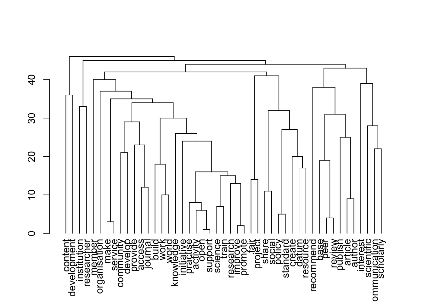
| Version | Author | Date |
|---|---|---|
| 796aa8e | zuzannazagrodzka | 2022-09-21 |
| Version | Author | Date |
|---|---|---|
| 796aa8e | zuzannazagrodzka | 2022-09-21 |
[1] 32 32
[1] "funders"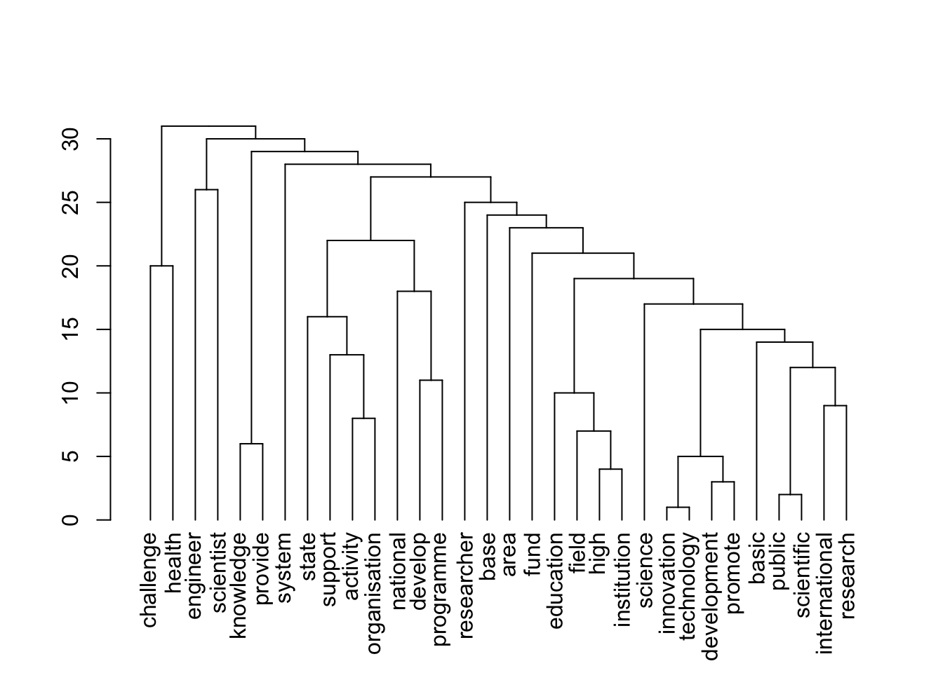
| Version | Author | Date |
|---|---|---|
| 796aa8e | zuzannazagrodzka | 2022-09-21 |
| Version | Author | Date |
|---|---|---|
| 796aa8e | zuzannazagrodzka | 2022-09-21 |
[1] 39 39
[1] "journals"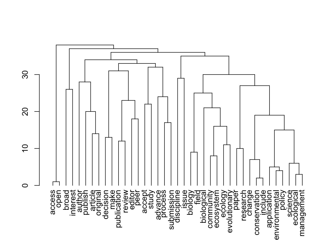
| Version | Author | Date |
|---|---|---|
| 796aa8e | zuzannazagrodzka | 2022-09-21 |
| Version | Author | Date |
|---|---|---|
| 796aa8e | zuzannazagrodzka | 2022-09-21 |
[1] 48 48
[1] "publishers"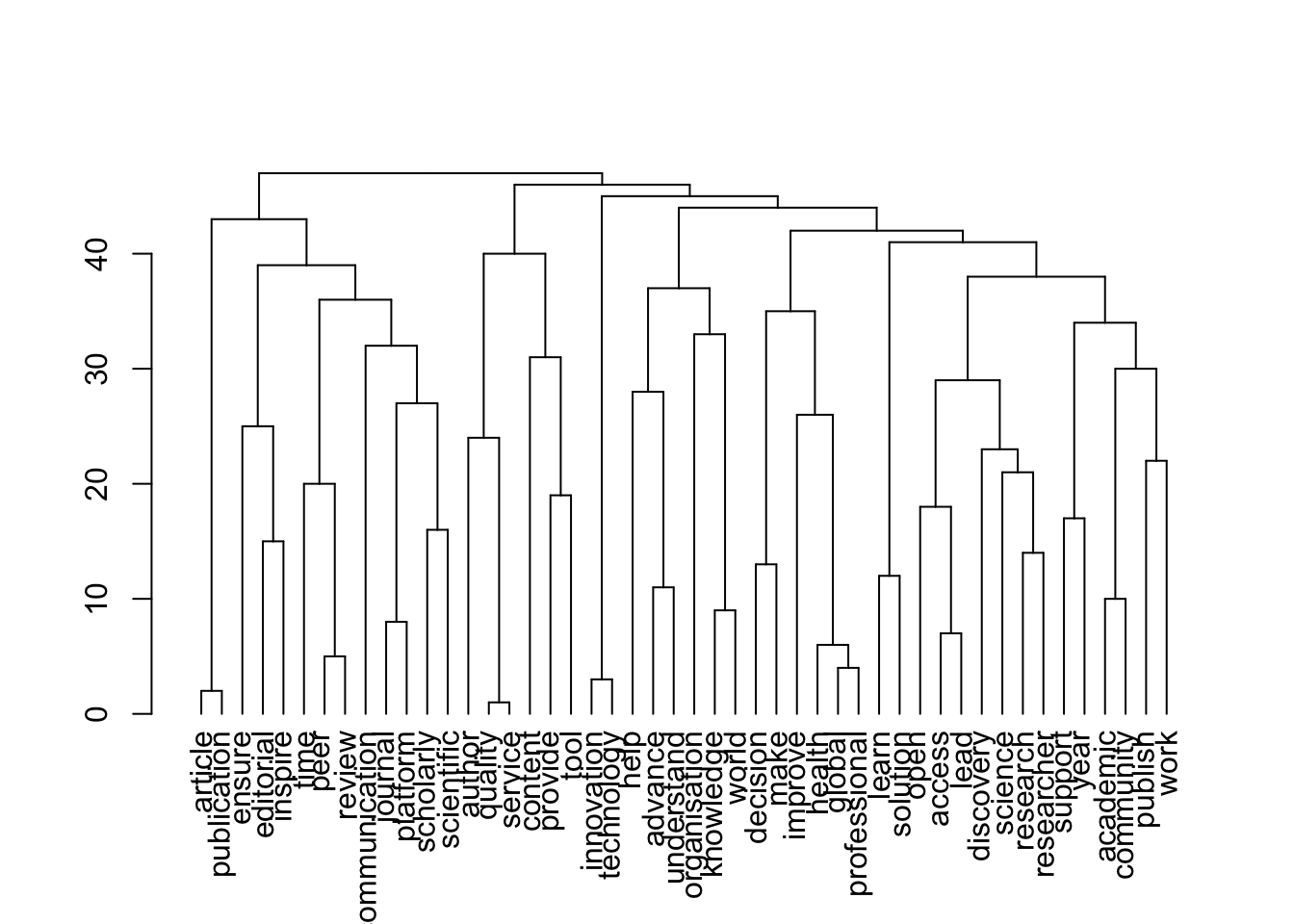
| Version | Author | Date |
|---|---|---|
| 796aa8e | zuzannazagrodzka | 2022-09-21 |
| Version | Author | Date |
|---|---|---|
| 796aa8e | zuzannazagrodzka | 2022-09-21 |
[1] 35 35
[1] "repositories"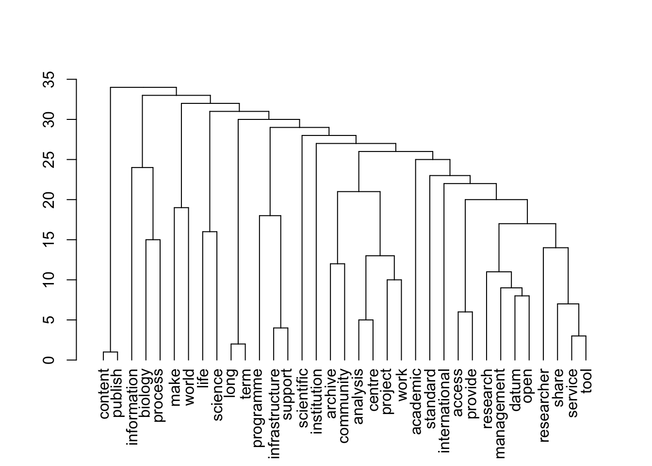
| Version | Author | Date |
|---|---|---|
| 796aa8e | zuzannazagrodzka | 2022-09-21 |
| Version | Author | Date |
|---|---|---|
| 796aa8e | zuzannazagrodzka | 2022-09-21 |
[1] 34 34
[1] "societies"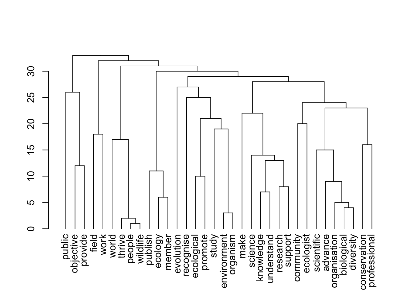
| Version | Author | Date |
|---|---|---|
| 796aa8e | zuzannazagrodzka | 2022-09-21 |
| Version | Author | Date |
|---|---|---|
| 796aa8e | zuzannazagrodzka | 2022-09-21 |
# Saving figures individually

figure_list
[1] "advocates_figure2B" "funders_figure2B" "journals_figure2B"
[4] "publishers_figure2B" "repositories_figure2B" "societies_figure2B" figure_name <- paste0("./output/Figure_2B/advocates_5topics_figure2B.png")
png(file=figure_name,
width= 3000, height= 3000, res=400)
advocates_figure2B
dev.off()quartz_off_screen
2 figure_name <- paste0("./output/Figure_2B/funders_5topics_figure2B.png")
png(file=figure_name,
width= 3000, height= 3000, res=400)
funders_figure2B
dev.off()quartz_off_screen
2 figure_name <- paste0("./output/Figure_2B/journals_5topics_figure2B.png")
png(file=figure_name,
width= 3000, height= 3000, res=400)
journals_figure2B
dev.off()quartz_off_screen
2 figure_name <- paste0("./output/Figure_2B/publishers_5topics_figure2B.png")
png(file=figure_name,
width= 3000, height= 3000, res=400)
publishers_figure2B
dev.off()quartz_off_screen
2 figure_name <- paste0("./output/Figure_2B/repositories_5topics_figure2B.png")
png(file=figure_name,
width= 3000, height= 3000, res=400)
repositories_figure2B
dev.off()quartz_off_screen
2 figure_name <- paste0("./output/Figure_2B/societies_5topics_figure2B.png")
png(file=figure_name,
width= 3000, height= 3000, res=400)
societies_figure2B
dev.off()quartz_off_screen
2 Additional analysis
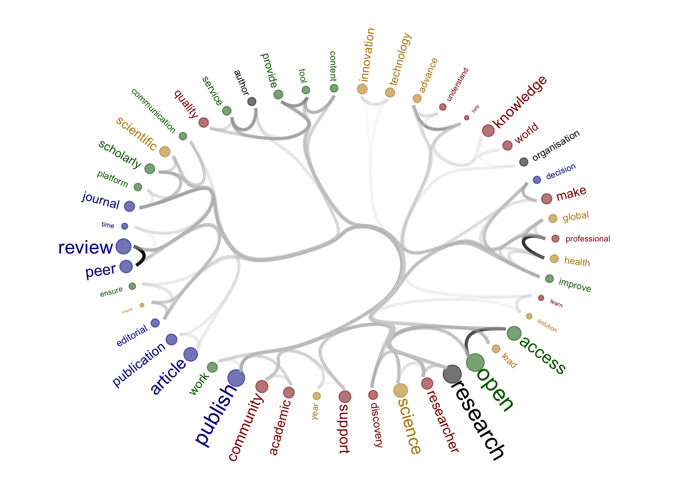
Circular graph created on all documents (all stakeholders)
# selecting data with the right name of the stakeholder
dat <- corpus_df %>%
  select(sentence_doc, word) %>%
  rename(id = sentence_doc)

  # Calculating similarity matrix
  cos_mat <- cosine_matrix(dat, lower = 0.035, upper = 1, filt = 0.9)

# Getting words used in the network
word_list_net <- rownames(cos_mat)
grep("workflow", word_list_net)integer(0)# Creating a graph
g <- graph_from_adjacency_matrix(cos_mat, mode = "undirected", weighted = TRUE)
topics = walktrap_topics(g)
plot(topics$dendrogram)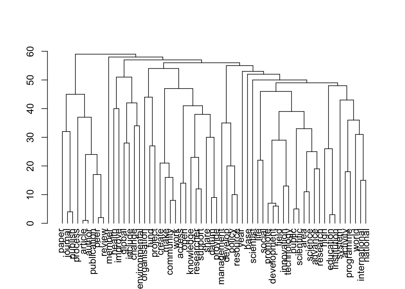
| Version | Author | Date |
|---|---|---|
| 796aa8e | zuzannazagrodzka | 2022-09-21 |
subtrees <- partition_leaves(topics$dendrogram)
leaves <- subtrees[[1]]

pathRoutes <- function(leaf) {
  which(sapply(subtrees, function(x) leaf %in% x))
}

paths <- lapply(leaves, pathRoutes)

edges = NULL
for(a in 1:length(paths)){
  # print(a)
  for(b in c(1:(length(paths[[a]])-1))){
    if(b == (length(paths[[a]])-1)){
      tmp_df = data.frame(
        from = paths[[a]][b],
        to = leaves[a]
      )
    } else {
      tmp_df = data.frame(
        from = paths[[a]][b],
        to = paths[[a]][b+1]
      )
    }
    edges = rbind(edges, tmp_df)
  }
}
connect = melt(cos_mat)
colnames(connect) = c("from", "to", "value")
connect = subset(connect, value != 0)


# create a vertices data.frame. One line per object of our hierarchy
vertices  <-  data.frame(
  name = unique(c(as.character(edges$from), as.character(edges$to)))
)
# Let's add a column with the group of each name. It will be useful later to color points
vertices$group  <-  edges$from[ match( vertices$name, edges$to ) ]


#Let's add information concerning the label we are going to add: angle, horizontal adjustement and potential flip
#calculate the ANGLE of the labels
#vertices$id <- NA
#myleaves <- which(is.na( match(vertices$name, edges$from) ))
#nleaves <- length(myleaves)
#vertices$id[ myleaves ] <- seq(1:nleaves)
#vertices$angle <- 90 - 360 * vertices$id / nleaves

# calculate the alignment of labels: right or left
# If I am on the left part of the plot, my labels have currently an angle < -90
#vertices$hjust <- ifelse( vertices$angle < -90, 1, 0)

# flip angle BY to make them readable
#vertices$angle <- ifelse(vertices$angle < -90, vertices$angle+180, vertices$angle)

# replacing "group" value with the topic numer from the STM

# Colour words by topic modelling topics (STM)
# I have to change the group numbers in topics

stm_top <- corpus_df %>%
  select(word, topic = topic)

stm_top$topic <- as.factor(stm_top$topic)
stm_top <- unique(stm_top)

# Removing group column and creating a new one based on the stm info
vertices <- vertices

vertices <- vertices %>%
  left_join(stm_top, by = c("name" = "word")) %>%
  select(-group) %>%
  rename(group = topic)

# Adding a beta value so I can use it in the graph
stm_beta <- corpus_df %>%
  select(word, beta = highest_mean_beta)
stm_beta <- unique(stm_beta)
dim(stm_beta)
[1] 2832 2vertices <- vertices %>%
left_join(stm_beta, by = c("name" = "word"))
vertices$beta_size = vertices$beta
##########################################################
# Create a graph object
mygraph <- igraph::graph_from_data_frame(edges, vertices=vertices)
# The connection object must refer to the ids of the leaves:
from <- match( connect$from, vertices$name)
to <- match( connect$to, vertices$name)
# Basic usual argument
tmp_plt = ggraph(mygraph, layout = 'dendrogram', circular = T) +
geom_node_point(aes(filter = leaf, x = x*1.05, y=y*1.05, alpha=0.2), size =0, colour = "white") +
#colour=group, size=value
scale_colour_manual(values= c("dark green", "dark red", "darkgoldenrod", "dark blue", "black"), na.value = "black") +
geom_conn_bundle(data = get_con(from = from, to = to, col = connect$value), tension = 0.9, aes(colour = col, alpha = col+0.5), width = 1.1) +
scale_edge_color_continuous(low="white", high="black") +
# geom_node_text(aes(x = x*1.1, y=y*1.1, filter = leaf, label=name, angle = angle, hjust=hjust), size=5, alpha=1) +
geom_node_text(aes(x = x*1.1, y=y*1.1, filter = leaf, label=name, colour = group, angle = 0, hjust = 0.5, size = beta_size), alpha=1) +
theme_void() +
theme(
legend.position="none",
plot.margin=unit(c(0,0,0,0),"cm"),
) +
expand_limits(x = c(-1.5, 1.5), y = c(-1.5, 1.5))
g <- ggplot_build(tmp_plt)
tmp_dat = g[[3]]$data
tmp_dat$position = NA
tmp_dat_a = subset(tmp_dat, x >= 0)
tmp_dat_a = tmp_dat_a[order(-tmp_dat_a$y),]
tmp_dat_a = subset(tmp_dat_a, !is.na(beta))
tmp_dat_a$order = 1:nrow(tmp_dat_a)
tmp_dat_b = subset(tmp_dat, x < 0)
tmp_dat_b = tmp_dat_b[order(-tmp_dat_b$y),]
tmp_dat_b = subset(tmp_dat_b, !is.na(beta))
tmp_dat_b$order = (nrow(tmp_dat_a) +nrow(tmp_dat_b)) : (nrow(tmp_dat_a) +1)
tmp_dat = rbind(tmp_dat_a, tmp_dat_b)
vertices = left_join(vertices, tmp_dat[,c("name", "order")], by = c("name"))
vert_save = vertices
vertices = vert_save
vertices$id <- NA
vertices = vertices[order(vertices$order),]
myleaves <- which(is.na( match(vertices$name, edges$from) ))
nleaves <- length(myleaves)
vertices$id[ myleaves ] <- seq(1:nleaves)
vertices$angle <- 90 - 360 * vertices$id / nleaves
# calculate the alignment of labels: right or left
# If I am on the left part of the plot, my labels have currently an angle < -90
vertices$hjust <- ifelse( vertices$angle < -90, 1, 0)
# flip angle BY to make them readable
vertices$angle <- ifelse(vertices$angle < -90, vertices$angle+180, vertices$angle)
vertices = vertices[order(as.numeric(rownames(vertices))),]
mygraph <- igraph::graph_from_data_frame(edges, vertices=vertices)
figure_tosave <- ggraph(mygraph, layout = 'dendrogram', circular = T) +
geom_node_point(aes(filter = leaf, x = x*1.05, y=y*1.05, alpha=0.2, colour = group, size = beta_size)) +
#colour=group, size=value
scale_colour_manual(values= c("dark green", "dark red", "darkgoldenrod", "dark blue", "black"), na.value = "black") +
geom_conn_bundle(data = get_con(from = from, to = to, col = connect$value), tension = 0.99, aes(colour = col, alpha = col+0.5), width = 1.1) +
scale_edge_color_continuous(low="grey90", high="black") +
geom_node_text(aes(x = x*1.1, y=y*1.1, filter = leaf, label=name, colour = group, angle = angle, hjust = hjust, size = beta_size)) +
theme_void() +
theme(
legend.position="none",
plot.margin=unit(c(0,0,0,0),"cm"),
) +
expand_limits(x = c(-1.6, 1.6), y = c(-1.6, 1.6))
figure_name <- paste0("./output/Other_figures/All_stakeholders_5topics_figure.png")
png(file=figure_name,
width=3000, height=3000, res = 500)
figure_tosave
dev.off()quartz_off_screen
2 figure_tosave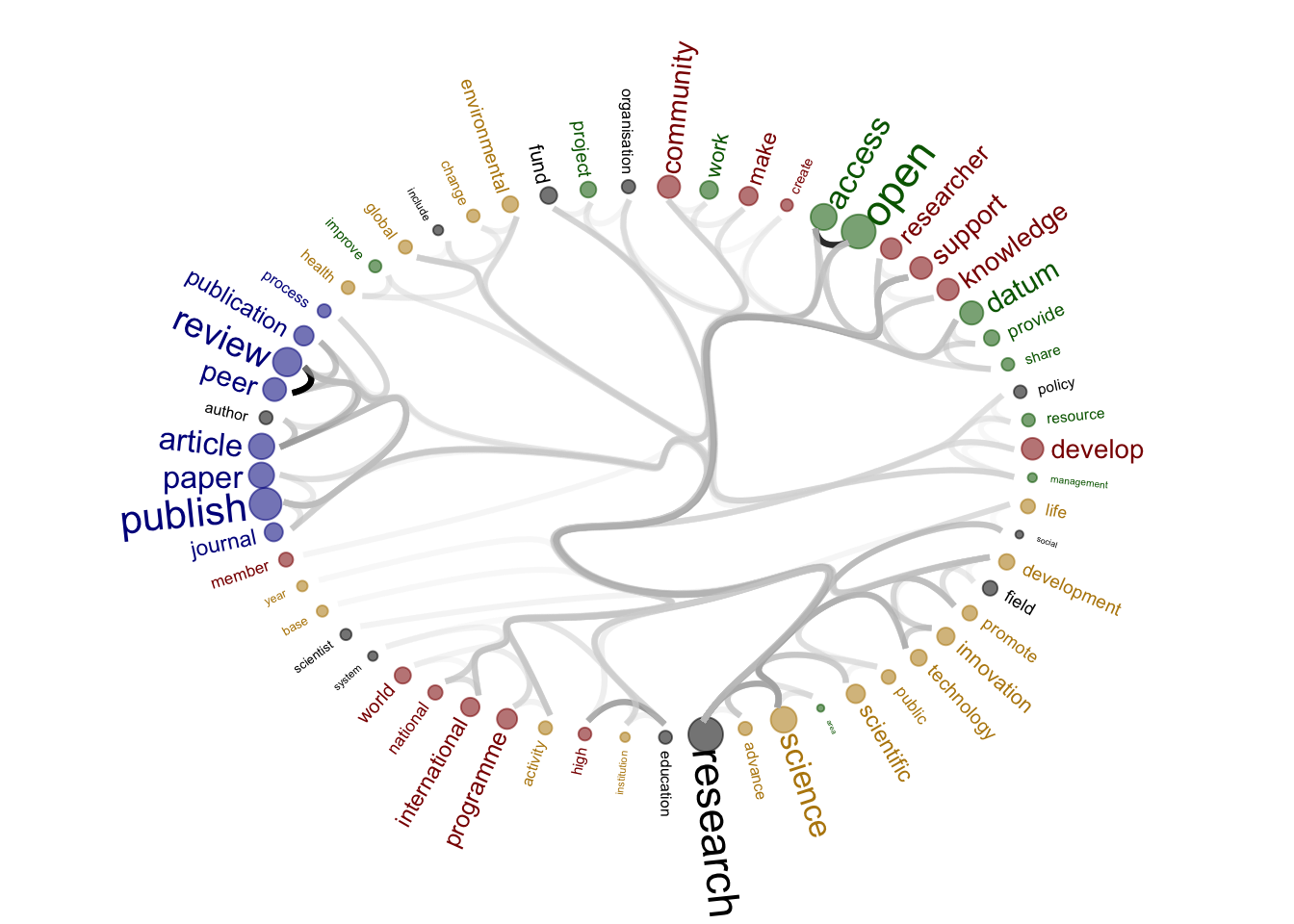
| Version | Author | Date |
|---|---|---|
| 796aa8e | zuzannazagrodzka | 2022-09-21 |
Session information
sessionInfo()R version 4.0.3 (2020-10-10)
Platform: x86_64-apple-darwin17.0 (64-bit)
Running under: macOS Big Sur 10.16
Matrix products: default
BLAS: /Library/Frameworks/R.framework/Versions/4.0/Resources/lib/libRblas.dylib
LAPACK: /Library/Frameworks/R.framework/Versions/4.0/Resources/lib/libRlapack.dylib
locale:
[1] en_GB.UTF-8/en_GB.UTF-8/en_GB.UTF-8/C/en_GB.UTF-8/en_GB.UTF-8
attached base packages:
[1] stats graphics grDevices utils datasets methods base
other attached packages:
[1] tidytext_0.3.2 forcats_0.5.1 stringr_1.4.0 purrr_0.3.4
[5] readr_2.0.2 tidyr_1.1.4 tibble_3.1.6 tidyverse_1.3.1
[9] dplyr_1.0.7 reshape2_1.4.4 ggraph_2.0.5 ggplot2_3.3.5
[13] igraph_1.2.6 dendextend_1.15.3 workflowr_1.7.0
loaded via a namespace (and not attached):
[1] lsa_0.73.2 fs_1.5.0 lubridate_1.7.10 httr_1.4.2
[5] rprojroot_2.0.2 SnowballC_0.7.0 tools_4.0.3 backports_1.2.1
[9] bslib_0.3.0 utf8_1.2.2 R6_2.5.1 DBI_1.1.1
[13] colorspace_2.0-2 withr_2.4.2 tidyselect_1.1.1 gridExtra_2.3
[17] processx_3.5.2 compiler_4.0.3 git2r_0.29.0 cli_3.1.0
[21] rvest_1.0.1 xml2_1.3.2 labeling_0.4.2 sass_0.4.0
[25] scales_1.1.1 callr_3.7.0 digest_0.6.28 rmarkdown_2.11
[29] pkgconfig_2.0.3 htmltools_0.5.2 highr_0.9 dbplyr_2.1.1
[33] fastmap_1.1.0 rlang_0.4.12 readxl_1.3.1 rstudioapi_0.13
[37] jquerylib_0.1.4 farver_2.1.0 generics_0.1.1 jsonlite_1.7.2
[41] tokenizers_0.2.1 magrittr_2.0.3 Matrix_1.3-4 Rcpp_1.0.7
[45] munsell_0.5.0 fansi_0.5.0 viridis_0.6.1 lifecycle_1.0.1
[49] stringi_1.7.5 whisker_0.4 yaml_2.2.1 MASS_7.3-54
[53] plyr_1.8.6 grid_4.0.3 promises_1.2.0.1 ggrepel_0.9.1
[57] crayon_1.4.2 lattice_0.20-45 graphlayouts_0.7.1 haven_2.4.3
[61] hms_1.1.1 knitr_1.36 ps_1.6.0 pillar_1.6.4
[65] reprex_2.0.1 glue_1.5.0 evaluate_0.14 getPass_0.2-2
[69] modelr_0.1.8 vctrs_0.3.8 tzdb_0.1.2 tweenr_1.0.2
[73] httpuv_1.6.3 cellranger_1.1.0 gtable_0.3.0 polyclip_1.10-0
[77] assertthat_0.2.1 xfun_0.31 ggforce_0.3.3 broom_0.7.9
[81] tidygraph_1.2.0 janeaustenr_0.1.5 later_1.3.0 viridisLite_0.4.0
[85] ellipsis_0.3.2