Bayesian Inference

Introduction
Bayes theorem
- Derivation of Bayes theorem
- Applying Bayes theorem: Example of screening test
Likelihoods and Likelihood ratios
- Likelihood vs probability
Likelihood ratios
Bayesian inference

Last updated: 2019-05-27

Checks: 6 0

Knit directory: MSTPsummerstatistics/

This reproducible R Markdown analysis was created with workflowr (version 1.3.0). The Checks tab describes the reproducibility checks that were applied when the results were created. The Past versions tab lists the development history.

R Markdown file: up-to-date

Great! Since the R Markdown file has been committed to the Git repository, you know the exact version of the code that produced these results.

Environment: empty

Great job! The global environment was empty. Objects defined in the global environment can affect the analysis in your R Markdown file in unknown ways. For reproduciblity it’s best to always run the code in an empty environment.

Seed: set.seed(20180927)

The command set.seed(20180927) was run prior to running the code in the R Markdown file. Setting a seed ensures that any results that rely on randomness, e.g. subsampling or permutations, are reproducible.

Session information: recorded

Great job! Recording the operating system, R version, and package versions is critical for reproducibility.

Cache: none

Nice! There were no cached chunks for this analysis, so you can be confident that you successfully produced the results during this run.

Repository version: c3c7b6e

Great! You are using Git for version control. Tracking code development and connecting the code version to the results is critical for reproducibility. The version displayed above was the version of the Git repository at the time these results were generated.

Note that you need to be careful to ensure that all relevant files for the analysis have been committed to Git prior to generating the results (you can use wflow_publish or wflow_git_commit). workflowr only checks the R Markdown file, but you know if there are other scripts or data files that it depends on. Below is the status of the Git repository when the results were generated:


Ignored files:
    Ignored:    .DS_Store
    Ignored:    .Rhistory
    Ignored:    .Rproj.user/
    Ignored:    analysis/.RData
    Ignored:    analysis/.Rhistory

Note that any generated files, e.g. HTML, png, CSS, etc., are not included in this status report because it is ok for generated content to have uncommitted changes.

These are the previous versions of the R Markdown and HTML files. If you’ve configured a remote Git repository (see ?wflow_git_remote), click on the hyperlinks in the table below to view them.

File	Version	Author	Date	Message
Rmd	c3c7b6e	Anthony Hung	2019-05-27	Bayesian
html	c3c7b6e	Anthony Hung	2019-05-27	Bayesian
html	b291d24	Anthony Hung	2019-05-24	Build site.
Rmd	a321d7b	Anthony Hung	2019-05-24	commit before republish
html	a321d7b	Anthony Hung	2019-05-24	commit before republish
html	c4bdfdc	Anthony Hung	2019-05-22	Build site.
Rmd	dd1e411	Anthony Hung	2019-05-22	before republishing syllabus
html	096760a	Anthony Hung	2019-05-18	Build site.
html	da98ae8	Anthony Hung	2019-05-17	Build site.
Rmd	239723e	Anthony Hung	2019-05-08	Update learning objectives
Rmd	8860e57	Anthony Hung	2019-05-06	Finalized schedule for classes
html	8860e57	Anthony Hung	2019-05-06	Finalized schedule for classes

Introduction

Bayesian inference is a fancy term for educated guessing. In essesence, in Bayesian inference we take prior information that we know about the world and use it to evaluate data that we are presented with to draw educated conclusions about the world.

Our objectives today include learning about Bayes theorem and its connections to conditional probability, likelihood ratios for comparing specified models, and applying Bayes theorem to inference problems.

Bayes theorem

Before we delve into Bayesian inference, we must first start by covering Bayes Theorem. Bayes Theorem is a result that comes from probability and describes the relationship between conditional probabilities.

Let us define A and B as two separate types of events. P(A|B), or “the probability of A given B” denotes the conditional probability of A occurring if we know that B has occurred. Likewise, P(B|A) denotes “the probability of B given A”. Bayes theorem relates P(A|B) and P(B|A) in a deceptively simple equation.

Derivation of Bayes theorem

https://oracleaide.files.wordpress.com/2012/12/ovals_pink_and_blue1.png

From our definition of conditional probability, we know that P(A|B) can be defined as the probability that A occurs given that B has occured. This can be written mathematically as:

\[P(A|B) = \frac{P(A \cap B )}{P(B)}\]

Here, \(\cap\) denotes the intersection between A and B (i.e. “A AND B occur together”). To calculate the probability of A conditional on B, we first need to find the probability that B has occured. Then, we need to figure out out of the situations where B has occured, how often does A also occur?

In a similar way, we can write P(B|A) mathematically:

\[P(B|A) = \frac{P(B \cap A )}{P(A)}\]

Since \(P(B \cap A )=P(A \cap B)\) (does this make sense?), we can combine the two equations:

\[P(A|B)P(B) = P(B \cap A ) = P(B|A)P(A)\]

If we divide both sides by P(B):

\[P(A|B) = \frac{P(B|A )P(A)}{P(B)}\]

This is Bayes theorem! Notice that using this equation, we can connect the two conditional probabilities. Oftentimes, knowing this relationship is extremely useful because we will know P(B|A) but want to compute P(A|B). Let’s explore an example.

Applying Bayes theorem: Example of screening test

Let us assume that a patient named John goes to a see a doctor to undergo a screening test for an infectious disease. The test that is performed has been previously researched, and it is known to have a 99% reliability when administered to patients like John. In other words, 99% of sick people test positive in the test and 99% of healthy people test negative. The doctor has prior knowledge that 1% of people in general will have the disease in question. If the patient tests positive, what are the chances that he is sick?

50%

Let’s solve this problem through applying Bayes theorem:

\[P(A|B) = \frac{P(B|A )P(A)}{P(B)}\]

First, we need to define what we mean by each of the terms as they relate to the question.

We can define P(A) as the probability that John is sick, and P(B) as the probability that John tests positive. If John is a normal every-day person, then we can use the Doctor’s knowledge that 1% of the population is sick as P(A).

P(A|B), the probability that John is sick given that he tests positive, is exactly what we want to calculate!

However, we are given only the other conditional probability, P(B|A) or the probability that a sick person tests positive (0.99).

Great. We have all the quantities we need to plug in to Bayes theorem to get our answer, except for P(B), the probability that a person tests positive. In order to calculate this, we can use the equation:

\[P(B) = P(B|A)P(A) + P(B| A^c)P(A^c)\]

Here, \(A^c\) denotes A not happening, in this case “John is not sick.” In essence, A can either be true or not, so the two terms should capture all possible scenarios where B can occur. In this case, what is \(P(B|A^c)\)?

\[P(A|B) = \frac{P(B|A )P(A)}{P(B|A)P(A) + P(B| A^c)P(A^c)}\]

Notice that the first term in the denominator is the same as the numerator. Let’s plug in our values and solve the problem.

\[P(A|B) = \frac{(0.99)(0.01)}{(0.99)(0.01) + (0.01)(0.99)} = \frac{1}{2}\]

Likelihoods and Likelihood ratios

Likelihood vs probability

Probability

Recall from our previous class on probability distributions that the definition of probability can be visualized as the area under the curve of a probability distribution. For example, let’s say that we have a fair coin (P(heads) = 0.5) and we flip it 30 times:

library(ggplot2)
library(cowplot)


Attaching package: 'cowplot'

The following object is masked from 'package:ggplot2':

    ggsave

library(grid)

x1  <- 5:25
df <- data.frame(x = x1, y = dbinom(x1, 30, 0.5))

ggplot(df, aes(x = x, y = y)) + 
  geom_bar(stat = "identity", col = "red", fill = c("white")) +
  scale_y_continuous(expand = c(0.01, 0)) + xlab("number of heads") + ylab("Density")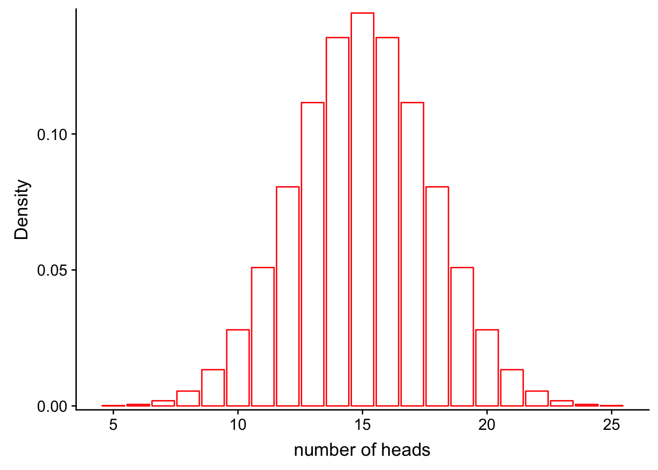

Version	Author	Date
c3c7b6e	Anthony Hung	2019-05-27

If we would like to find the probability that we would get more than 20 heads in 30 flips, we could calculate the area represented by bars that are greater than 18 on the x axis:

ggplot(df, aes(x = x, y = y)) + 
  geom_bar(stat = "identity", col = "red", fill = c(rep("white", 14), rep("red", 7))) +
  scale_y_continuous(expand = c(0.01, 0)) + xlab("number of heads") + ylab("Density")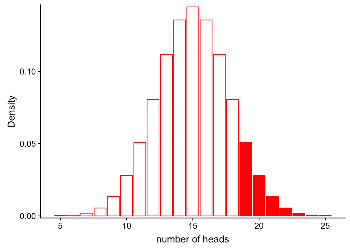

Version	Author	Date
c3c7b6e	Anthony Hung	2019-05-27

Similarly, we could calculate the probability that we get between 9 and 13 heads:

ggplot(df, aes(x = x, y = y)) + 
  geom_bar(stat = "identity", col = "red", fill = c(rep("white", 5), rep("red", 4), rep("white", 12))) +
  scale_y_continuous(expand = c(0.01, 0)) + xlab("number of heads") + ylab("Density")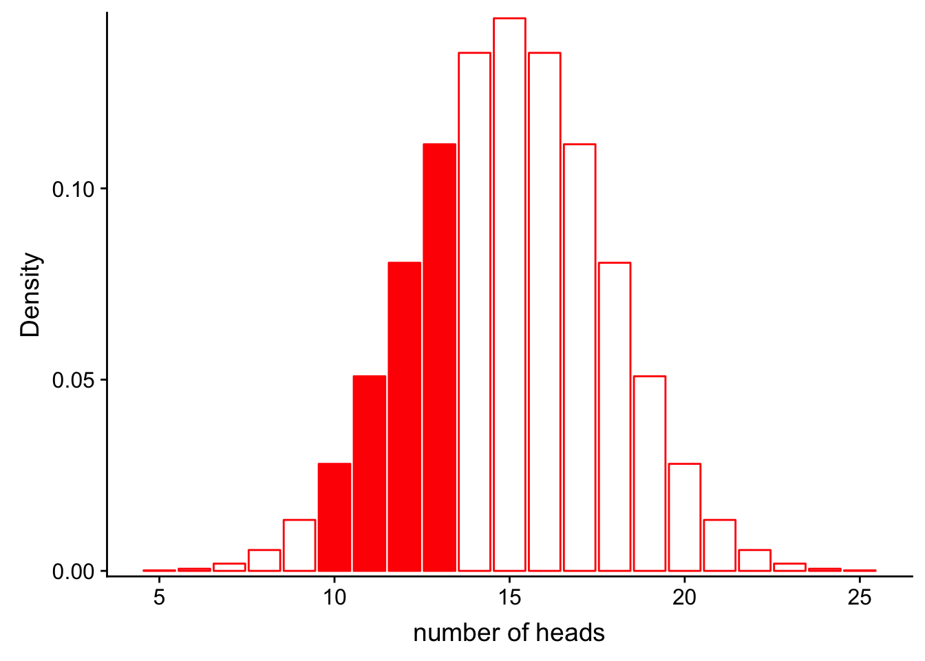

Version	Author	Date
c3c7b6e	Anthony Hung	2019-05-27

In each case, notice that the shape of the distribution does not change. The only thing that changes is the area that we shade in. In mathematical terms, in the first case we are calculating:

\[P(num\_heads > 20 | Binom(n=30, p=0.5))\]

and in the second:

\[P(9< num\_heads < 13 | Binom(n=30, p=0.5))\]

What is changing is the left side of the | . The shape of the distribution stays the same. When we discuss probabilities, we are talking about the areas under a fixed distribution (model).

Likelihood

So what about likelihood? Before we look at it graphically, let’s define what we mean by the term. “The likelihood for a model is the probability of the data under the model.” Mathematically,

\[L(Model|Data) = P(Data|Model)\]

This may look the same as what we did before, but in this case our data are fixed, not the distribution. Instead of asking, “If I keep my distribution constant, what is the probability of observing something?” with likelihood we are asking “Given that I have collected some data, how well does a certain distribution fit the data?”

Let’s assume the same situation we did for probability with the coin. In this case, we do not know if the coin is actually fair (P(heads = 0.5), or if it is rigged (e.g. P(heads = 0.6). We flip the coin 30 times and observe 20 heads.

What is the likelihood for our fair model (\(Binom(n=30, p=0.5)\)) given that we observe these data? In other words, how well does the model as paramterized fit our observations?

\[L(Model|Data) = P(num\_heads = 20|Binom(n=30, p=0.5))\]

Let’s look at this graphically.

ggplot(df, aes(x = x, y = y)) + 
  geom_bar(stat = "identity", col = "red", fill = c(rep("white", 15), rep("red", 1), rep("white", 5))) +
  scale_y_continuous(expand = c(0.01, 0)) + xlab("number of heads") + ylab("Density")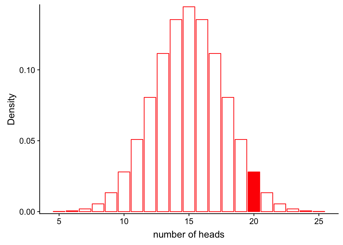

Version	Author	Date
c3c7b6e	Anthony Hung	2019-05-27

We can also compute the exact probability using the “dbinom” function in R.

dbinom(x = 20, size = 30, prob = 0.5)

[1] 0.0279816

Okay. How well does our data fit a rigged coin model, where the P(heads = 0.6)? What is the likelihood for the rigged coin model given our data?

\[L(Model|Data) = P(num\_heads = 25|Binom(n=30, p=0.6))\]

Let’s look at this graphically.

x1  <- 5:25
df_rigged <- data.frame(x = x1, y = dbinom(x1, 30, 0.6))

ggplot(df_rigged, aes(x = x, y = y)) + 
  geom_bar(stat = "identity", col = "red", fill = c(rep("white", 15), rep("red", 1), rep("white", 5))) +
  scale_y_continuous(expand = c(0.01, 0)) + xlab("number of heads") + ylab("Density")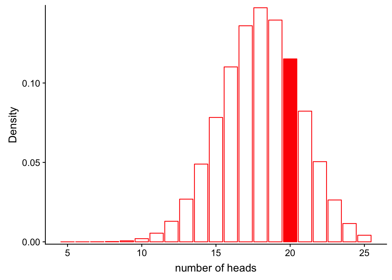

Version	Author	Date
c3c7b6e	Anthony Hung	2019-05-27

We can also compute the exact probability using the “dbinom” function in R.

dbinom(x = 20, size = 30, prob = 0.6)

[1] 0.1151854

It looks like the likelihood for the rigged coin model is higher! But is it high enough for us to say that the coin is rigged? Under both models, the probability of obtaining 20 heads is not that high, and we may want to base our conclusions on more robust statistics than a simple “it’s higher, therefore it’s true” heuristic. One way we can compare likelihoods is through likelihood ratios.

Likelihood ratios