Integration and clustering of scRNA sequencing data
Anthony Hung
2021-01-19
Last updated: 2021-01-26
Checks: 6 1
Knit directory: invitroOA_pilot_repository/
This reproducible R Markdown analysis was created with workflowr (version 1.6.2). The Checks tab describes the reproducibility checks that were applied when the results were created. The Past versions tab lists the development history.
The R Markdown file has unstaged changes. To know which version of the R Markdown file created these results, you’ll want to first commit it to the Git repo. If you’re still working on the analysis, you can ignore this warning. When you’re finished, you can run wflow_publish to commit the R Markdown file and build the HTML.
Great job! The global environment was empty. Objects defined in the global environment can affect the analysis in your R Markdown file in unknown ways. For reproduciblity it’s best to always run the code in an empty environment.
The command set.seed(20210119) was run prior to running the code in the R Markdown file. Setting a seed ensures that any results that rely on randomness, e.g. subsampling or permutations, are reproducible.
Great job! Recording the operating system, R version, and package versions is critical for reproducibility.
Nice! There were no cached chunks for this analysis, so you can be confident that you successfully produced the results during this run.
Great job! Using relative paths to the files within your workflowr project makes it easier to run your code on other machines.
Great! You are using Git for version control. Tracking code development and connecting the code version to the results is critical for reproducibility.
The results in this page were generated with repository version 833430f. See the Past versions tab to see a history of the changes made to the R Markdown and HTML files.
Note that you need to be careful to ensure that all relevant files for the analysis have been committed to Git prior to generating the results (you can use wflow_publish or wflow_git_commit). workflowr only checks the R Markdown file, but you know if there are other scripts or data files that it depends on. Below is the status of the Git repository when the results were generated:
Ignored files:
    Ignored:    .Rhistory
    Ignored:    .Rproj.user/
    Ignored:    code/bulkRNA_preprocessing/.snakemake/conda-archive/
    Ignored:    code/bulkRNA_preprocessing/.snakemake/conda/
    Ignored:    code/bulkRNA_preprocessing/.snakemake/locks/
    Ignored:    code/bulkRNA_preprocessing/.snakemake/shadow/
    Ignored:    code/bulkRNA_preprocessing/.snakemake/singularity/
    Ignored:    code/bulkRNA_preprocessing/.snakemake/tmp.3ekfs3n5/
    Ignored:    code/bulkRNA_preprocessing/fastq/
    Ignored:    code/bulkRNA_preprocessing/out/
    Ignored:    code/single_cell_preprocessing/.snakemake/conda-archive/
    Ignored:    code/single_cell_preprocessing/.snakemake/conda/
    Ignored:    code/single_cell_preprocessing/.snakemake/locks/
    Ignored:    code/single_cell_preprocessing/.snakemake/shadow/
    Ignored:    code/single_cell_preprocessing/.snakemake/singularity/
    Ignored:    code/single_cell_preprocessing/YG-AH-2S-ANT-1_S1_L008/
    Ignored:    code/single_cell_preprocessing/YG-AH-2S-ANT-2_S2_L008/
    Ignored:    code/single_cell_preprocessing/demuxlet/.DS_Store
    Ignored:    code/single_cell_preprocessing/fastq/
    Ignored:    data/external_scRNA/Chou_et_al2020/
    Ignored:    data/external_scRNA/Jietal2018/
    Ignored:    data/external_scRNA/Wuetal2021/
    Ignored:    data/external_scRNA/merged_external_scRNA.rds
    Ignored:    data/poweranalysis/alasoo_et_al/
    Ignored:    output/GO_terms_enriched.csv
    Ignored:    output/topicModel_k=6.rds
    Ignored:    output/topicModel_k=7.rds
    Ignored:    output/topicModel_k=8.rds
    Ignored:    output/voom_results.rds

Unstaged changes:
    Modified:   .gitignore
    Modified:   analysis/clustering_scRNA.Rmd
Note that any generated files, e.g. HTML, png, CSS, etc., are not included in this status report because it is ok for generated content to have uncommitted changes.
These are the previous versions of the repository in which changes were made to the R Markdown (analysis/clustering_scRNA.Rmd) and HTML (docs/clustering_scRNA.html) files. If you’ve configured a remote Git repository (see ?wflow_git_remote), click on the hyperlinks in the table below to view the files as they were in that past version.
| File | Version | Author | Date | Message |
|---|---|---|---|---|
| html | 8542407 | Anthony Hung | 2021-01-21 | knit anlaysis files |
| Rmd | 0ef10b1 | Anthony Hung | 2021-01-21 | warning = F |
| html | 0ef10b1 | Anthony Hung | 2021-01-21 | warning = F |
| Rmd | 9cf26dc | Anthony Hung | 2021-01-21 | suppress warnings |
| html | 9cf26dc | Anthony Hung | 2021-01-21 | suppress warnings |
| Rmd | d7cac01 | Anthony Hung | 2021-01-21 | load more libraries |
| Rmd | 5e6c873 | Anthony Hung | 2021-01-21 | load ggplot2 |
| Rmd | 37a702d | Anthony Hung | 2021-01-21 | add clustering details |
| Rmd | 78cfbcd | Anthony Hung | 2021-01-21 | finish paring down files |
| Rmd | 99c70b8 | Anthony Hung | 2021-01-20 | update external data |
| Rmd | d6b5b17 | Anthony Hung | 2021-01-20 | Added analysis files |
| Rmd | 28f57fa | Anthony Hung | 2021-01-19 | Add files for analysis |
Introduction
To determine cell type heterogeneity between samples jointly, this code treats each individual (unstrained condition) as its own separate sample and performs integration across individuals. It then finds clusters within the integrated data and characterizes the clusters.
Load data and packages
The ANT1.2 seurat object was generated by running the preprocessing code in Pre-processing of raw 10x files into count matrices and demultiplexing.
library(Seurat)
library(gridExtra)
library(ggplot2)
library(cowplot)
library(tidyverse)
Registered S3 method overwritten by 'cli':
method from
print.boxx spatstat── Attaching packages ────────────────────────────────── tidyverse 1.3.0 ──✓ tibble 3.0.4 ✓ dplyr 1.0.2
✓ tidyr 1.1.2 ✓ stringr 1.4.0
✓ readr 1.3.1 ✓ forcats 0.4.0
✓ purrr 0.3.4 ── Conflicts ───────────────────────────────────── tidyverse_conflicts() ──
x dplyr::combine() masks gridExtra::combine()
x dplyr::filter() masks stats::filter()
x dplyr::lag() masks stats::lag()library(ashr)
library(Matrix)
Attaching package: 'Matrix'The following objects are masked from 'package:tidyr':
expand, pack, unpackANT1.2 <- readRDS("data/ANT1_2.rds")Split data into individuals
First, we split the merged seurat object into separate objects corresponding to the individual from which cells originated. Then integrate across the individuals using SCT transform
#split data into each individual/sample
NA18855_Unstrain <- subset(ANT1.2, labels == "NA18855_Unstrain")
NA18856_Unstrain <- subset(ANT1.2, labels == "NA18856_Unstrain")
NA19160_Unstrain <- subset(ANT1.2, labels == "NA19160_Unstrain")

# Create a seurat object merged for all the unstrain samples (because we are missing one individual for the strained samples)
seurat.list <- list(NA18855_Unstrain, NA18856_Unstrain, NA19160_Unstrain)
for (i in 1:length(seurat.list)) {
    seurat.list[[i]] <- SCTransform(seurat.list[[i]], verbose = FALSE)
}

SCT.features <- SelectIntegrationFeatures(object.list = seurat.list, nfeatures = 5000)
seurat.list <- PrepSCTIntegration(object.list = seurat.list, anchor.features = SCT.features,
    verbose = FALSE)

#find anchors
seurat.anchors <- FindIntegrationAnchors(object.list = seurat.list, normalization.method = "SCT",
    anchor.features = SCT.features, verbose = FALSE)
SCT.integrated <- IntegrateData(anchorset = seurat.anchors, normalization.method = "SCT",
    verbose = FALSE)

#visualized integrated
SCT.integrated <- RunPCA(SCT.integrated, verbose = FALSE, npcs = 100)
DimPlot(SCT.integrated, reduction = "pca", group.by = c("labels"))
| Version | Author | Date |
|---|---|---|
| 9cf26dc | Anthony Hung | 2021-01-21 |
ElbowPlot(SCT.integrated, ndims = 100) #38 PCs?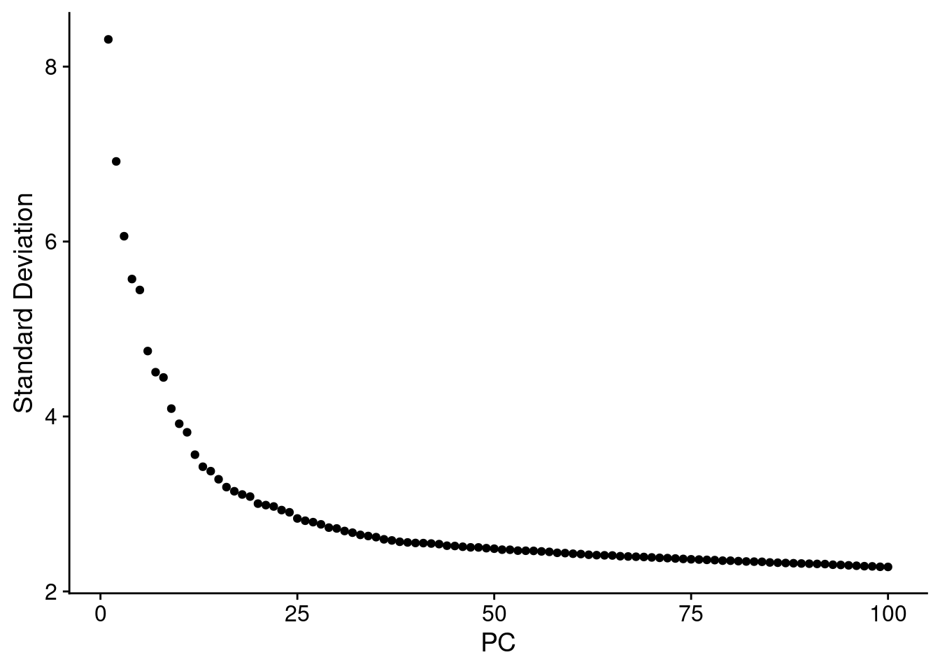
| Version | Author | Date |
|---|---|---|
| 9cf26dc | Anthony Hung | 2021-01-21 |
SCT.integrated <- FindNeighbors(SCT.integrated, dims = 1:38)Computing nearest neighbor graphComputing SNNSCT.integrated <- FindClusters(SCT.integrated, resolution = 0.4)Modularity Optimizer version 1.3.0 by Ludo Waltman and Nees Jan van Eck
Number of nodes: 1203
Number of edges: 67564
Running Louvain algorithm...
Maximum modularity in 10 random starts: 0.6657
Number of communities: 3
Elapsed time: 0 secondsDimPlot(SCT.integrated, group.by = c("labels"), reduction = "pca")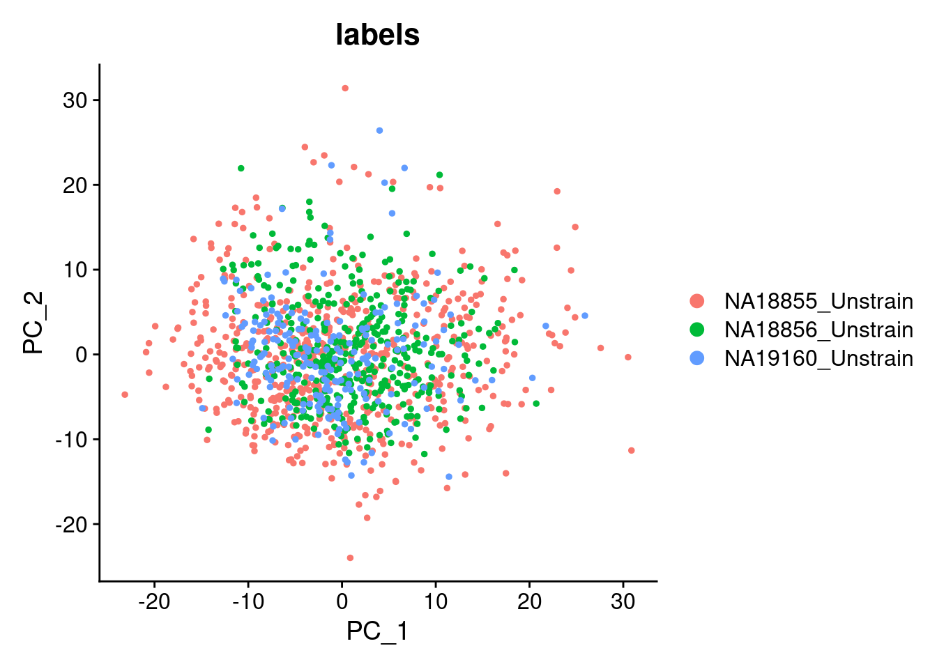
| Version | Author | Date |
|---|---|---|
| 9cf26dc | Anthony Hung | 2021-01-21 |
DimPlot(SCT.integrated, group.by = c("seurat_clusters"), reduction = "pca")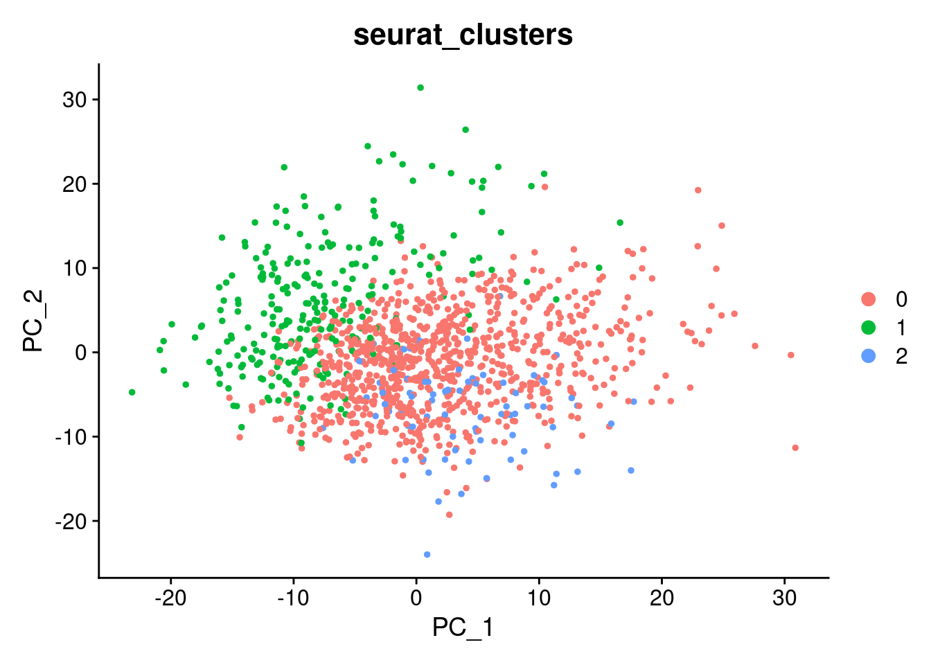
| Version | Author | Date |
|---|---|---|
| 9cf26dc | Anthony Hung | 2021-01-21 |
SCT.integrated <- RunUMAP(SCT.integrated, dims = 1:38)21:05:46 UMAP embedding parameters a = 0.9922 b = 1.11221:05:46 Read 1203 rows and found 38 numeric columns21:05:46 Using Annoy for neighbor search, n_neighbors = 3021:05:46 Building Annoy index with metric = cosine, n_trees = 500% 10 20 30 40 50 60 70 80 90 100%[----|----|----|----|----|----|----|----|----|----|**************************************************|
21:05:46 Writing NN index file to temp file /tmp/RtmpVstoIG/file2f0197c684e6a
21:05:46 Searching Annoy index using 1 thread, search_k = 3000
21:05:46 Annoy recall = 100%
21:05:47 Commencing smooth kNN distance calibration using 1 thread
21:05:47 Initializing from normalized Laplacian + noise
21:05:48 Commencing optimization for 500 epochs, with 45058 positive edges
21:05:51 Optimization finishedp1_SCT <- DimPlot(SCT.integrated, group.by = c("orig.ident"))
p2_SCT <- DimPlot(SCT.integrated, group.by = c("labels"))
p3_SCT <- DimPlot(SCT.integrated, group.by = c("seurat_clusters"))
grid.arrange(p1_SCT, p2_SCT, p3_SCT, nrow = 2)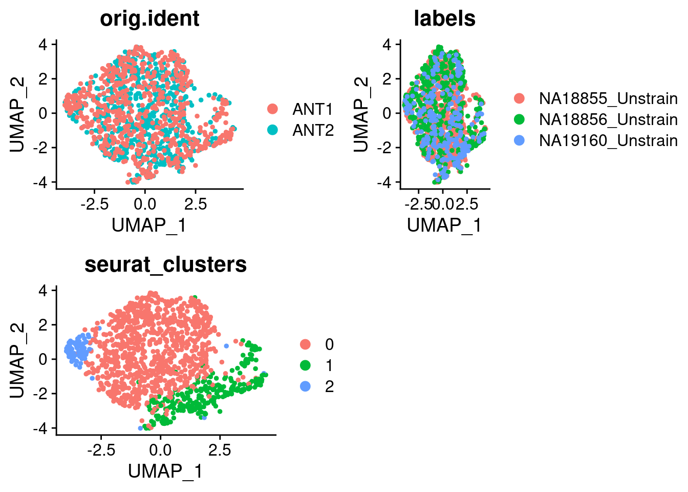
| Version | Author | Date |
|---|---|---|
| 9cf26dc | Anthony Hung | 2021-01-21 |
#for figures: remove legend and add in later
p1_figure <- p2_SCT + theme(legend.position = "none")
p2_figure <- p3_SCT + theme(legend.position = "none") + scale_color_manual(values=c("plum3", "#E69F00", "#654321"))
grid.arrange(p1_figure, p2_figure)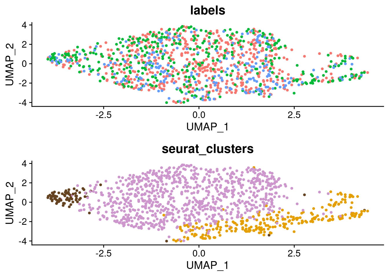
| Version | Author | Date |
|---|---|---|
| 9cf26dc | Anthony Hung | 2021-01-21 |
p2_SCT 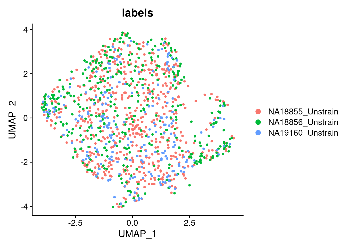
| Version | Author | Date |
|---|---|---|
| 9cf26dc | Anthony Hung | 2021-01-21 |
p3_SCT + scale_color_manual(values=c("plum3", "#E69F00", "#654321"))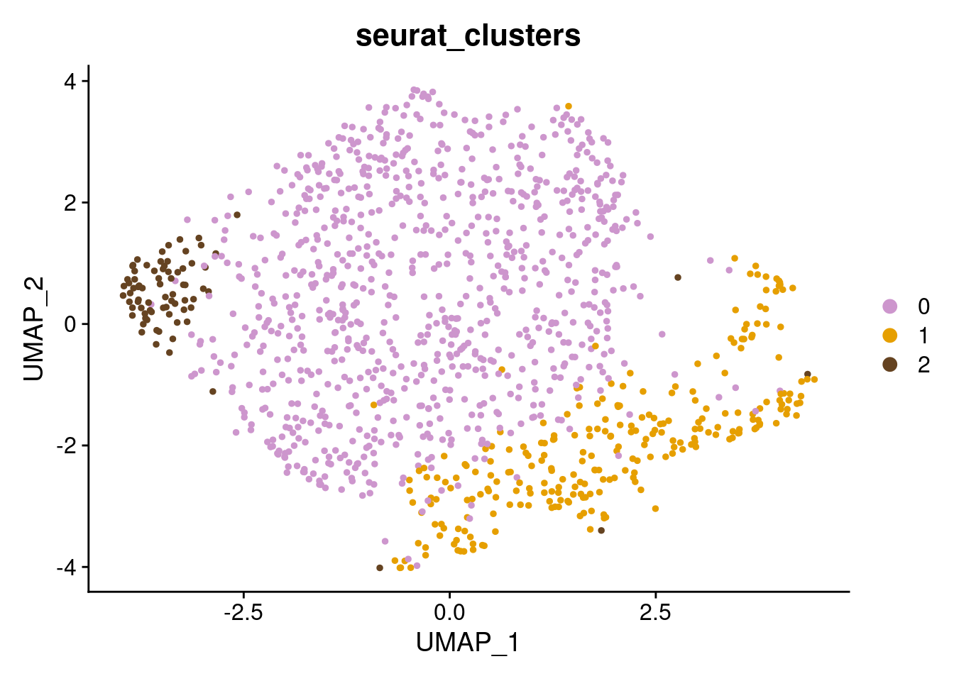
| Version | Author | Date |
|---|---|---|
| 9cf26dc | Anthony Hung | 2021-01-21 |
SCT.integrated@active.ident <- SCT.integrated$integrated_snn_res.0.4Examine clusters in integrated data
We identified 3 clusters in the integrated data. We now characterize them by gene expression for a chondrogenic marker gene to get a sense of which cluster(s) represent more mature chondrocytes.
cluster_memberships <- as.matrix(table(SCT.integrated@meta.data$integrated_snn_res.0.4, SCT.integrated@meta.data$labels))
cluster_memberships
    NA18855_Unstrain NA18856_Unstrain NA19160_Unstrain
  0              429              280              156
  1              129               81               51
  2               28               34               15
cluster_memberships_proportions <- prop.table(cluster_memberships, margin = 2)
cluster_memberships_proportions
    NA18855_Unstrain NA18856_Unstrain NA19160_Unstrain
  0       0.73208191       0.70886076       0.70270270
  1       0.22013652       0.20506329       0.22972973
  2       0.04778157       0.08607595       0.06756757
#make a nice proportions bar plot for a figure
long_cluster_memberships_proportions <- as_tibble(as.data.frame(cluster_memberships_proportions))
ggplot(long_cluster_memberships_proportions, aes(x = Var2, y = Freq, fill = Var1)) +
geom_bar(position = "dodge", stat = "identity") +
scale_fill_manual(values=c("plum3", "#E69F00", "#654321")) +
theme_cowplot() +
labs(title = "Proportion of cells from each individual \n assigned to each unsupervised cluster", x = "", y = "Proportion", fill = "Cluster")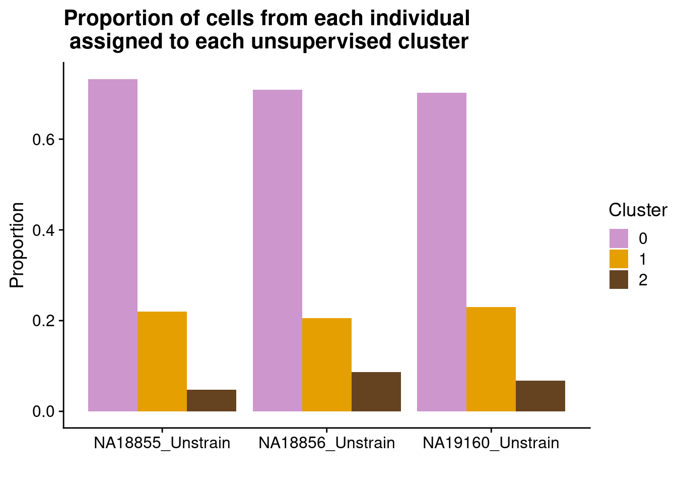
| Version | Author | Date |
|---|---|---|
| 9cf26dc | Anthony Hung | 2021-01-21 |
Explore some cluster marker genes
Here, we fit a poisson ash model to raw counts from each of the three clusters for chondrocyte marker genes and plot their distributions broken down by cluster and by individual.
#run poisson ash to data per cluster and per indivdiual, then show the estimated prior distribution
#plot curves for genes separated by indivdual (information for indivdual contained in labels)
plot_by_labels <- function(gene, counts, labels){
     #create dataframe to store the cdf axes and the groups
     dataframe_cdf <- data.frame(x = c(), y = c(), label = c())
     for(individual in unique(labels)){ #in the case that the labels supplied contain cluster, it will do this by cluster instead
          x <- counts[gene, labels == individual]
          s <- colSums(counts[,labels == individual]) #sum of molecule counts per sample
          lam <- x/s
          fit <- ashr::ash_pois(x, s, mixcompdist = "halfuniform")
          cdf <- ashr::cdf.ash(fit, seq(from = 0, to = max(lam), length.out = 1000))
          temp_df <- cbind(cdf$x, t(cdf$y), individual)
          names(temp_df) <- c("x", "y", "label")
          dataframe_cdf <- rbind(dataframe_cdf, temp_df)
     }
     names(dataframe_cdf) <- c("x", "y", "label")
     dataframe_cdf$x <- as.character(dataframe_cdf$x)
     dataframe_cdf$y <- as.character(dataframe_cdf$y)
     dataframe_cdf$x <- as.numeric(dataframe_cdf$x)
     dataframe_cdf$y <- as.numeric(dataframe_cdf$y)
     #use df to make our plot
     plot <- ggplot(dataframe_cdf, aes(x = x, y = y, color = as.factor(label), group=as.factor(label))) +
          geom_point() +
          labs(title = paste0(gene), x = "Latent gene expression", y = "CDF", color = "Label") +
          theme_cowplot()
     return(plot)
}


#plots for figures
#COL11A1
a <- plot_by_labels("COL11A1", SCT.integrated@assays$RNA@counts, SCT.integrated$integrated_snn_res.0.4) +
     theme(legend.position = "none") +
     scale_color_manual(values=c("plum3", "#E69F00", "#654321"))
b <- plot_by_labels("COL11A1", SCT.integrated@assays$RNA@counts, SCT.integrated$labels) +
     theme(legend.position = "none")
grid.arrange(a, b, nrow = 1)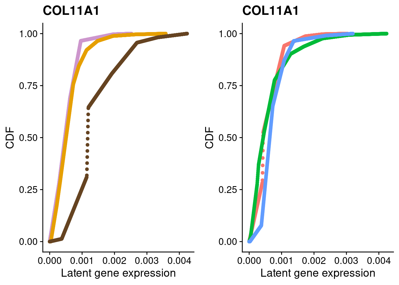
| Version | Author | Date |
|---|---|---|
| 9cf26dc | Anthony Hung | 2021-01-21 |
#SOX5
a <- plot_by_labels("SOX5", SCT.integrated@assays$RNA@counts, SCT.integrated$integrated_snn_res.0.4) +
     theme(legend.position = "none") +
     scale_color_manual(values=c("plum3", "#E69F00", "#654321"))
b <- plot_by_labels("SOX5", SCT.integrated@assays$RNA@counts, SCT.integrated$labels) +
     theme(legend.position = "none")
grid.arrange(a, b, nrow = 1)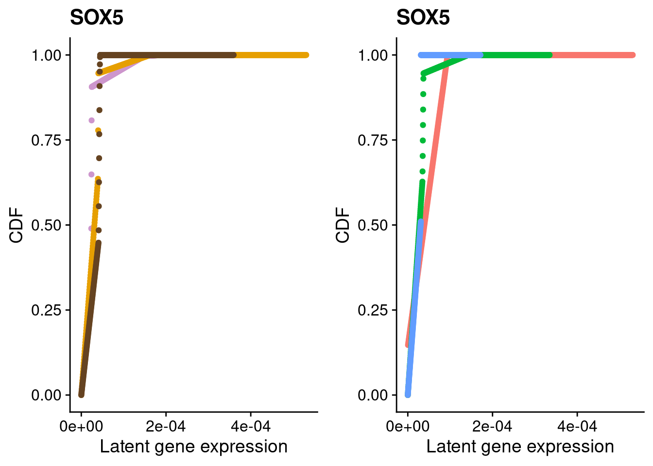
| Version | Author | Date |
|---|---|---|
| 9cf26dc | Anthony Hung | 2021-01-21 |
#SOX6
a <- plot_by_labels("SOX6", SCT.integrated@assays$RNA@counts, SCT.integrated$integrated_snn_res.0.4) +
     theme(legend.position = "none") +
     scale_color_manual(values=c("plum3", "#E69F00", "#654321"))
b <- plot_by_labels("SOX6", SCT.integrated@assays$RNA@counts, SCT.integrated$labels) +
     theme(legend.position = "none")
grid.arrange(a, b, nrow = 1)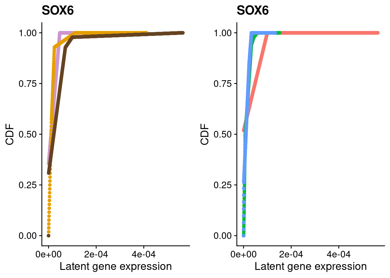
| Version | Author | Date |
|---|---|---|
| 9cf26dc | Anthony Hung | 2021-01-21 |
#TIMP2
a <- plot_by_labels("TIMP2", SCT.integrated@assays$RNA@counts, SCT.integrated$integrated_snn_res.0.4) +
     theme(legend.position = "none") +
     scale_color_manual(values=c("plum3", "#E69F00", "#654321"))
b <- plot_by_labels("TIMP2", SCT.integrated@assays$RNA@counts, SCT.integrated$labels) +
     theme(legend.position = "none")
grid.arrange(a, b, nrow = 1)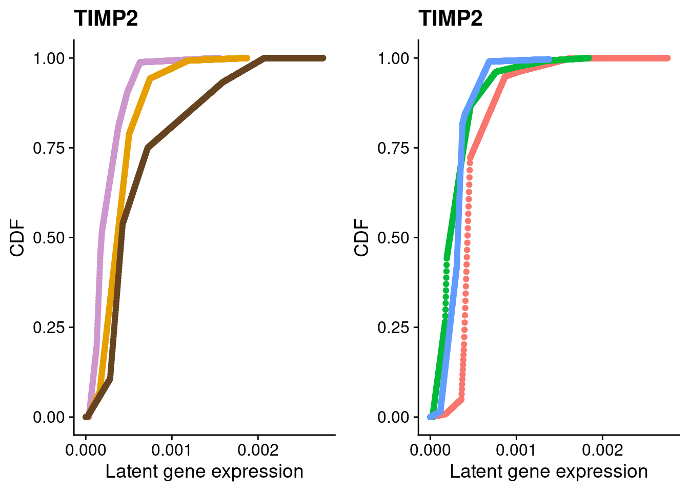
| Version | Author | Date |
|---|---|---|
| 9cf26dc | Anthony Hung | 2021-01-21 |
#TIMP3
a <- plot_by_labels("TIMP3", SCT.integrated@assays$RNA@counts, SCT.integrated$integrated_snn_res.0.4) +
     theme(legend.position = "none") +
     scale_color_manual(values=c("plum3", "#E69F00", "#654321"))
b <- plot_by_labels("TIMP3", SCT.integrated@assays$RNA@counts, SCT.integrated$labels) +
     theme(legend.position = "none")
grid.arrange(a, b, nrow = 1)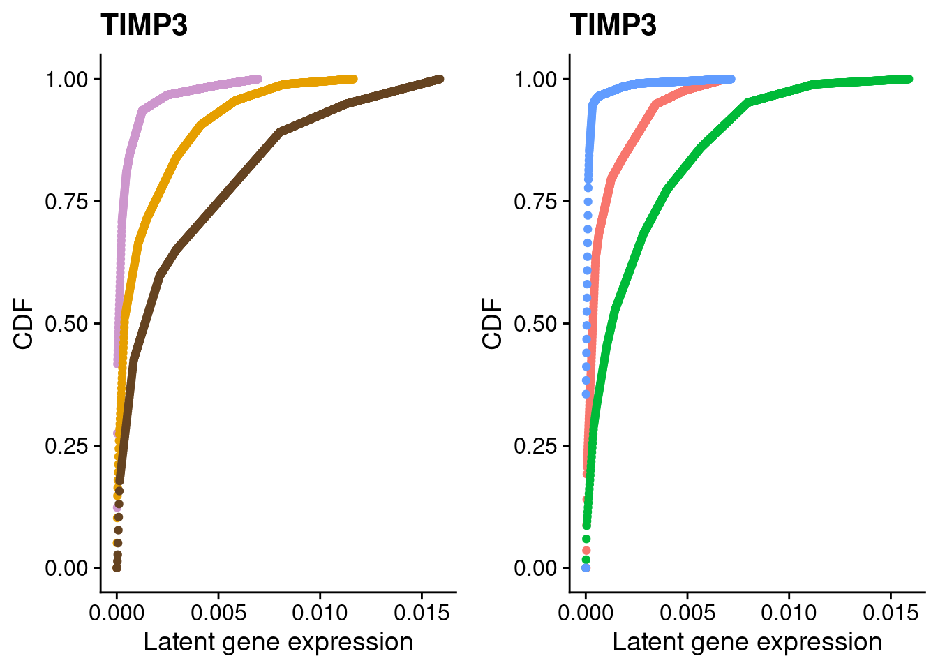
| Version | Author | Date |
|---|---|---|
| 9cf26dc | Anthony Hung | 2021-01-21 |
sessionInfo()R version 3.6.1 (2019-07-05)
Platform: x86_64-pc-linux-gnu (64-bit)
Running under: Scientific Linux 7.4 (Nitrogen)
Matrix products: default
BLAS/LAPACK: /software/openblas-0.2.19-el7-x86_64/lib/libopenblas_haswellp-r0.2.19.so
locale:
[1] LC_CTYPE=en_US.UTF-8 LC_NUMERIC=C
[3] LC_TIME=en_US.UTF-8 LC_COLLATE=en_US.UTF-8
[5] LC_MONETARY=en_US.UTF-8 LC_MESSAGES=en_US.UTF-8
[7] LC_PAPER=en_US.UTF-8 LC_NAME=C
[9] LC_ADDRESS=C LC_TELEPHONE=C
[11] LC_MEASUREMENT=en_US.UTF-8 LC_IDENTIFICATION=C
attached base packages:
[1] stats graphics grDevices utils datasets methods base
other attached packages:
[1] Matrix_1.2-18 ashr_2.2-47 forcats_0.4.0 stringr_1.4.0
[5] dplyr_1.0.2 purrr_0.3.4 readr_1.3.1 tidyr_1.1.2
[9] tibble_3.0.4 tidyverse_1.3.0 cowplot_1.1.0 ggplot2_3.3.3
[13] gridExtra_2.3 Seurat_3.2.3
loaded via a namespace (and not attached):
[1] readxl_1.3.1 backports_1.1.10 workflowr_1.6.2
[4] plyr_1.8.6 igraph_1.2.4.1 lazyeval_0.2.2
[7] splines_3.6.1 listenv_0.8.0 scattermore_0.7
[10] digest_0.6.27 invgamma_1.1 htmltools_0.5.0
[13] SQUAREM_2020.4 gdata_2.18.0 fansi_0.4.1
[16] magrittr_2.0.1 tensor_1.5 cluster_2.1.0
[19] ROCR_1.0-7 globals_0.12.5 modelr_0.1.8
[22] matrixStats_0.57.0 colorspace_2.0-0 rvest_0.3.6
[25] rappdirs_0.3.1 ggrepel_0.9.0 haven_2.3.1
[28] xfun_0.8 crayon_1.3.4 jsonlite_1.7.2
[31] spatstat_1.64-1 spatstat.data_1.7-0 survival_2.44-1.1
[34] zoo_1.8-8 glue_1.4.2 polyclip_1.10-0
[37] gtable_0.3.0 leiden_0.3.1 future.apply_1.3.0
[40] abind_1.4-5 scales_1.1.1 DBI_1.1.0
[43] miniUI_0.1.1.1 Rcpp_1.0.5 viridisLite_0.3.0
[46] xtable_1.8-4 reticulate_1.16 rsvd_1.0.1
[49] truncnorm_1.0-8 htmlwidgets_1.5.2 httr_1.4.2
[52] gplots_3.0.1.1 RColorBrewer_1.1-2 ellipsis_0.3.1
[55] ica_1.0-2 farver_2.0.3 pkgconfig_2.0.3
[58] uwot_0.1.10 dbplyr_1.4.2 deldir_0.1-23
[61] labeling_0.4.2 tidyselect_1.1.0 rlang_0.4.10
[64] reshape2_1.4.3 later_1.1.0.1 munsell_0.5.0
[67] cellranger_1.1.0 tools_3.6.1 cli_2.2.0
[70] generics_0.0.2 broom_0.7.0 ggridges_0.5.1
[73] evaluate_0.14 yaml_2.2.1 goftest_1.2-2
[76] npsurv_0.4-0 knitr_1.23 fs_1.3.1
[79] fitdistrplus_1.0-14 caTools_1.17.1.2 RANN_2.6.1
[82] pbapply_1.4-0 future_1.18.0 nlme_3.1-140
[85] whisker_0.3-2 mime_0.9 xml2_1.3.2
[88] compiler_3.6.1 rstudioapi_0.13 plotly_4.9.2.1
[91] png_0.1-7 lsei_1.2-0 spatstat.utils_1.17-0
[94] reprex_0.3.0 stringi_1.4.6 RSpectra_0.15-0
[97] lattice_0.20-41 vctrs_0.3.6 pillar_1.4.7
[100] lifecycle_0.2.0 lmtest_0.9-37 RcppAnnoy_0.0.18
[103] data.table_1.13.0 bitops_1.0-6 irlba_2.3.3
[106] httpuv_1.5.1 patchwork_1.1.0 R6_2.5.0
[109] promises_1.1.1 KernSmooth_2.23-15 codetools_0.2-16
[112] MASS_7.3-52 gtools_3.8.1 assertthat_0.2.1
[115] rprojroot_2.0.2 withr_2.3.0 sctransform_0.3.2
[118] mgcv_1.8-28 parallel_3.6.1 hms_0.5.3
[121] grid_3.6.1 rpart_4.1-15 rmarkdown_1.13
[124] Rtsne_0.15 git2r_0.26.1 mixsqp_0.3-43
[127] shiny_1.3.2 lubridate_1.7.9