DEanalysis_bulkRNA
Anthony Hung
2021-01-19
Last updated: 2021-01-21
Checks: 6 1
Knit directory: invitroOA_pilot_repository/
This reproducible R Markdown analysis was created with workflowr (version 1.6.2). The Checks tab describes the reproducibility checks that were applied when the results were created. The Past versions tab lists the development history.
The R Markdown file has unstaged changes. To know which version of the R Markdown file created these results, you’ll want to first commit it to the Git repo. If you’re still working on the analysis, you can ignore this warning. When you’re finished, you can run wflow_publish to commit the R Markdown file and build the HTML.
Great job! The global environment was empty. Objects defined in the global environment can affect the analysis in your R Markdown file in unknown ways. For reproduciblity it’s best to always run the code in an empty environment.
The command set.seed(20210119) was run prior to running the code in the R Markdown file. Setting a seed ensures that any results that rely on randomness, e.g. subsampling or permutations, are reproducible.
Great job! Recording the operating system, R version, and package versions is critical for reproducibility.
Nice! There were no cached chunks for this analysis, so you can be confident that you successfully produced the results during this run.
Great job! Using relative paths to the files within your workflowr project makes it easier to run your code on other machines.
Great! You are using Git for version control. Tracking code development and connecting the code version to the results is critical for reproducibility.
The results in this page were generated with repository version 0ef10b1. See the Past versions tab to see a history of the changes made to the R Markdown and HTML files.
Note that you need to be careful to ensure that all relevant files for the analysis have been committed to Git prior to generating the results (you can use wflow_publish or wflow_git_commit). workflowr only checks the R Markdown file, but you know if there are other scripts or data files that it depends on. Below is the status of the Git repository when the results were generated:
Ignored files:
    Ignored:    .Rhistory
    Ignored:    .Rproj.user/
    Ignored:    code/bulkRNA_preprocessing/.snakemake/conda-archive/
    Ignored:    code/bulkRNA_preprocessing/.snakemake/conda/
    Ignored:    code/bulkRNA_preprocessing/.snakemake/locks/
    Ignored:    code/bulkRNA_preprocessing/.snakemake/shadow/
    Ignored:    code/bulkRNA_preprocessing/.snakemake/singularity/
    Ignored:    code/bulkRNA_preprocessing/.snakemake/tmp.3ekfs3n5/
    Ignored:    code/bulkRNA_preprocessing/fastq/
    Ignored:    code/bulkRNA_preprocessing/out/
    Ignored:    code/single_cell_preprocessing/.snakemake/conda-archive/
    Ignored:    code/single_cell_preprocessing/.snakemake/conda/
    Ignored:    code/single_cell_preprocessing/.snakemake/locks/
    Ignored:    code/single_cell_preprocessing/.snakemake/shadow/
    Ignored:    code/single_cell_preprocessing/.snakemake/singularity/
    Ignored:    code/single_cell_preprocessing/YG-AH-2S-ANT-1_S1_L008/
    Ignored:    code/single_cell_preprocessing/YG-AH-2S-ANT-2_S2_L008/
    Ignored:    code/single_cell_preprocessing/demuxlet/.DS_Store
    Ignored:    code/single_cell_preprocessing/fastq/
    Ignored:    data/external_scRNA/Chou_et_al2020/
    Ignored:    data/external_scRNA/Jietal2018/
    Ignored:    data/external_scRNA/Wuetal2021/
    Ignored:    data/external_scRNA/merged_external_scRNA.rds
    Ignored:    data/poweranalysis/alasoo_et_al/
    Ignored:    output/GO_terms_enriched.csv
    Ignored:    output/topicModel_k=7.rds
    Ignored:    output/voom_results.rds

Untracked files:
    Untracked:  analysis/figure/

Unstaged changes:
    Modified:   .gitignore
    Modified:   analysis/DEanalysis_bulkRNA.Rmd
Note that any generated files, e.g. HTML, png, CSS, etc., are not included in this status report because it is ok for generated content to have uncommitted changes.
These are the previous versions of the repository in which changes were made to the R Markdown (analysis/DEanalysis_bulkRNA.Rmd) and HTML (docs/DEanalysis_bulkRNA.html) files. If you’ve configured a remote Git repository (see ?wflow_git_remote), click on the hyperlinks in the table below to view the files as they were in that past version.
| File | Version | Author | Date | Message |
|---|---|---|---|---|
| Rmd | 78cfbcd | Anthony Hung | 2021-01-21 | finish paring down files |
| Rmd | e3fbd0f | Anthony Hung | 2021-01-21 | add ward et al data files to data |
| Rmd | 0711682 | Anthony Hung | 2021-01-21 | start normalization file |
| Rmd | 28f57fa | Anthony Hung | 2021-01-19 | Add files for analysis |
Introduction
This code takes as input the filtered count data and two factors of unwanted variation fit by RUVs. It then uses limma and voom to perform differential expression analysis between treatment conditions using the data. After we have a set of differentially expressed genes, we look for enrichments amongst DE genes in GO pathways and previously published osteoarthritis datasets.
Load libraries and data
library("limma")
library("plyr")
library("dplyr")
library("edgeR")
library("tidyr")
library("ashr")
library("ggplot2")
library("RUVSeq")
library("topGO")

#load in filtered count data, RUVs output
filt_counts <- readRDS("data/filtered_counts.rds")
filt_counts <- filt_counts$counts
RUVsOut <- readRDS("data/RUVsOut.rds")

# load gene annotations
gene_anno <- read.delim("data/gene-annotation.txt",
                        sep = "\t")

# load in reordered sample information
sampleinfo <- readRDS("data/Sample.info.RNAseq.reordered.rds")
Specify design matrix for Linear mixed model
anno <- pData(RUVsOut)
x <- paste0(anno$Individual, anno$treatment)

anno$LibraryPrepBatch <- factor(anno$LibraryPrepBatch, levels = c("1", "2"))
anno$Replicate <- factor(anno$Replicate, levels = c("1", "2", "3"))

design <- model.matrix(~treatment + Individual + W_1 + W_2 + RIN,
                       data = anno)
colnames(design) <- gsub("treatment", "", colnames(design))
colnames(design)
[1] "(Intercept)" "Unstrain" "IndividualNA18856 "
[4] "IndividualNA19160 " "W_1" "W_2"
[7] "RIN" # Model replicate as a random effect
# Recommended to run both voom and duplicateCorrelation twice.
# https://support.bioconductor.org/p/59700/#67620
#TMM Normalization
y <- DGEList(filt_counts)
y <- calcNormFactors(y, method = "TMM")
#Voom for differential expression
v1 <- voom(y, design)
corfit1 <- duplicateCorrelation(v1, design, block = x)Warning in glmgam.fit(dx, dy, coef.start = start, tol = tol, maxit =
maxit, : Too much damping - convergence tolerance not achievablecorfit1$consensus.correlation[1] 0.3550961v2 <- voom(y, design, block = x, correlation = corfit1$consensus.correlation)
corfit2 <- duplicateCorrelation(v2, design, block = x)Warning in glmgam.fit(dx, dy, coef.start = start, tol = tol, maxit =
maxit, : Too much damping - convergence tolerance not achievablecorfit2$consensus.correlation[1] 0.3552816fit <- lmFit(v2, design, block = x,
correlation = corfit2$consensus.correlation)
fit <- eBayes(fit)
saveRDS(v2, "output/voom_results.rds")Assess model results
get_results <- function(x, number = nrow(x$coefficients), sort.by = "none",
...) {
# x - object MArrayLM from eBayes output
# ... - additional arguments passed to topTable
stopifnot(class(x) == "MArrayLM")
results <- topTable(x, number = number, sort.by = sort.by, ...)
return(results)
}
top_treatment <- get_results(fit, coef = "Unstrain", sort.by = "B")
head(top_treatment) logFC AveExpr t P.Value adj.P.Val
ENSG00000102317 0.9649351 6.618275 9.783461 1.949206e-08 0.0002043938
ENSG00000104368 -3.0870735 3.752845 -7.948281 3.730563e-07 0.0019559341
ENSG00000100292 -1.1063623 5.399063 -7.094331 1.703017e-06 0.0054809583
ENSG00000080824 -0.5377509 8.888183 -6.532144 4.882916e-06 0.0054809583
ENSG00000133142 0.5626177 7.056136 6.518984 5.007395e-06 0.0054809583
ENSG00000181019 -0.7825629 5.824147 -6.484784 5.346514e-06 0.0054809583
B
ENSG00000102317 9.596620
ENSG00000104368 6.308490
ENSG00000100292 5.350899
ENSG00000080824 4.351922
ENSG00000133142 4.324081
ENSG00000181019 4.268181results_treatment <- get_results(fit, coef = "Unstrain",
number = nrow(filt_counts), sort = "none")
ma_treatment <- ggplot(data.frame(Amean = fit$Amean, logFC = fit$coef[, "Unstrain"]),
aes(x = Amean, y = logFC)) +
geom_point() +
labs(x = "Average expression level", y = "Log fold change",
title = "Treatment effect")
ma_treatment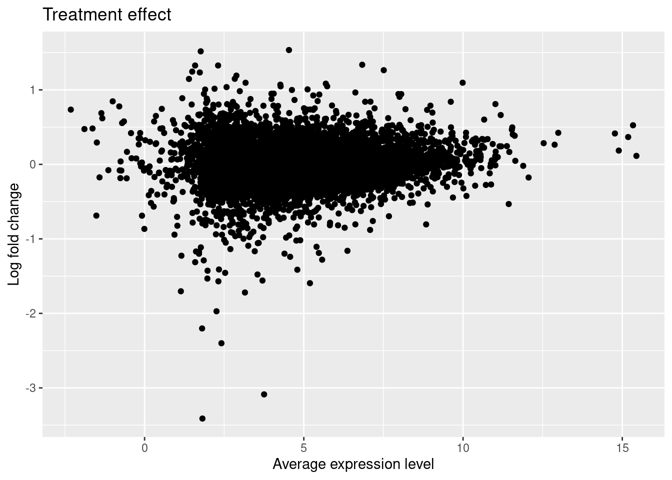
hist_treatment <- ggplot(results_treatment, aes(x = P.Value)) +
geom_histogram(binwidth = 0.01) +
labs(x = "p-value", y = "Number of genes", title = "Treatment effect")
hist_treatment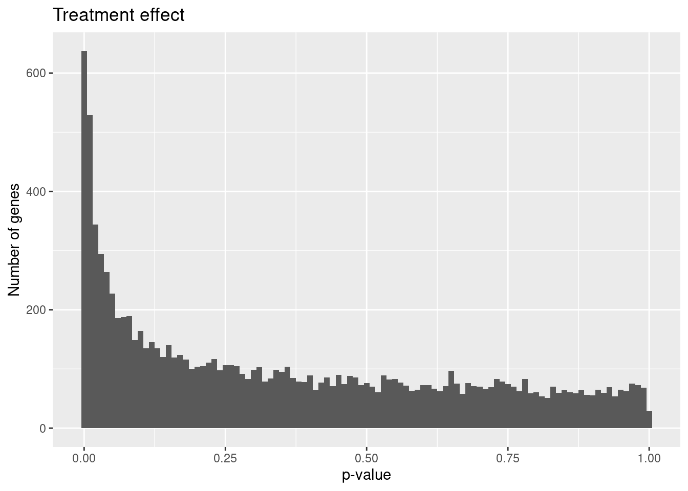
Use ash for mutliple testing correction
Treatment effect.
run_ash <- function(x, coef) {
# Perform multiple testing correction with adaptive shrinkage (ASH)
#
# x - object MArrayLM from eBayes output
# coef - coefficient tested by eBayes
stopifnot(class(x) == "MArrayLM", coef %in% colnames(x$coefficients))
result <- ash(betahat = x$coefficients[, coef],
sebetahat = x$stdev.unscaled[, coef] * sqrt(x$s2.post),
df = x$df.total[1])
return(result)
}
ash_treatment <- run_ash(fit, "Unstrain")
class(ash_treatment)[1] "ash"names(ash_treatment)[1] "fitted_g" "loglik" "logLR" "data" "result" "call" sum(ash_treatment$result$svalue < .05)[1] 773hist(ash_treatment$result$svalue)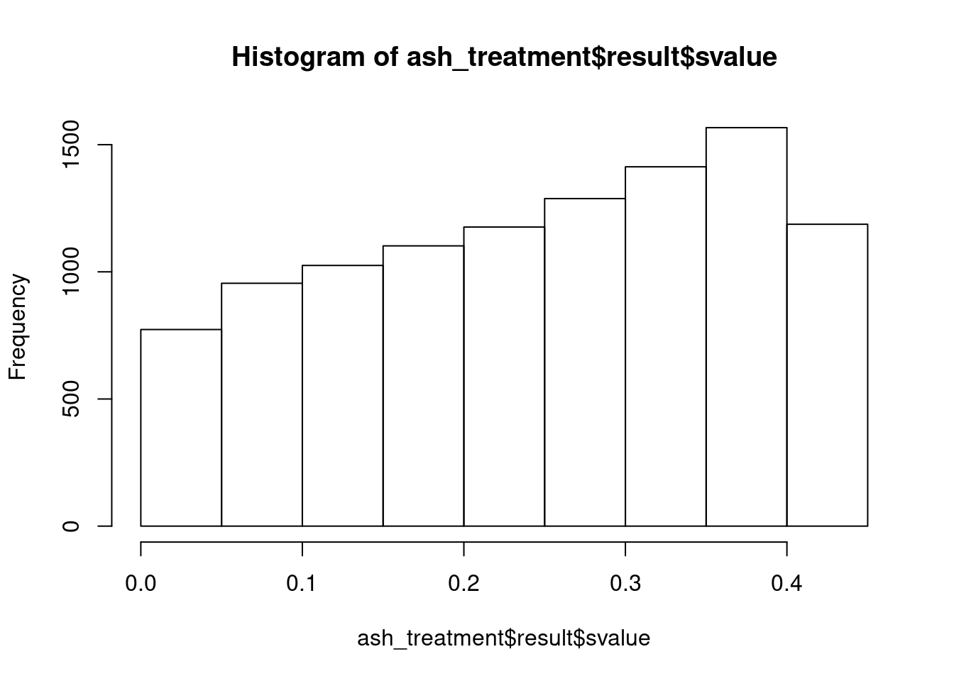
Plots
plot_ma <- function(x, qval) {
# Create MA plot.
#
# x - data frame with topTable and ASH output
# (columns logFC, AveExpr, and qvalue)
# qval - qvalue cutoff for calling a gene DE
#
stopifnot(is.data.frame(x), c("logFC", "AveExpr", "qvalue") %in% colnames(x),
is.numeric(qval), qval <= 1, qval >= 0)
x$highlight <- ifelse(x$qvalue < qval, "darkred", "gray75")
x$highlight <- factor(x$highlight, levels = c("darkred", "gray75"))
ggplot(x, aes(x = AveExpr, y = logFC, color = highlight, shape = highlight)) +
geom_point() +
labs(x = "Average expression level", y = "Log fold change") +
scale_color_identity(drop = FALSE) +
scale_shape_manual(values = c(16, 1), drop = FALSE) +
theme(legend.position = "none")
# scale_color_gradient(low = "red", high = "white", limits = c(0, 0.25))
}
plot_volcano <- function(x, qval) {
# Create volcano plot.
#
# x - data frame with topTable and ASH output
# (columns logFC, P.Value, and qvalue)
# qval - qvalue cutoff for calling a gene DE
#
stopifnot(is.data.frame(x), c("logFC", "P.Value", "qvalue") %in% colnames(x),
is.numeric(qval), qval <= 1, qval >= 0)
x$highlight <- ifelse(x$qvalue < qval, "darkred", "gray75")
x$highlight <- factor(x$highlight, levels = c("darkred", "gray75"))
ggplot(x, aes(x = logFC, y = -log10(P.Value), color = highlight)) +
geom_point(shape = 1) +
labs(x = "Log fold change",
y = expression(-log[10] * " p-value")) +
scale_color_identity(drop = FALSE) +
theme(legend.position = "none")
}
plot_pval_hist <- function(x, qval) {
# Create histogram of p-values.
#
# x - data frame with topTable and ash output (columns P.Value and qvalue)
# qval - qvalue cutoff for calling a gene DE
#
stopifnot(is.data.frame(x), c("P.Value", "qvalue") %in% colnames(x))
x$highlight <- ifelse(x$qvalue < qval, "darkred", "gray75")
x$highlight <- factor(x$highlight, levels = c("darkred", "gray75"))
ggplot(x, aes(x = P.Value, fill = highlight)) +
geom_histogram(position = "stack", binwidth = 0.01) +
scale_fill_identity(drop = FALSE) +
labs(x = "p-value", y = "Number of genes")
}tests <- colnames(fit$coefficients)
results <- vector(length = length(tests), mode = "list")
names(results) <- tests
for (test in tests[c(1:7)]) {
# Extract limma results
print(test)
results[[test]] <- get_results(fit, coef = test)
# Add mutliple testing correction with ASH
output_ash <- run_ash(fit, coef = test)$result
results[[test]] <- cbind(results[[test]], lfsr = output_ash$lfsr,
lfdr = output_ash$lfdr, qvalue = output_ash$qvalue,
svalue = output_ash$svalue)
}[1] "(Intercept)"
[1] "Unstrain"
[1] "IndividualNA18856 "
[1] "IndividualNA19160 "
[1] "W_1"
[1] "W_2"
[1] "RIN"#FDR 0.05
plot_ma(results[["Unstrain"]], 0.05)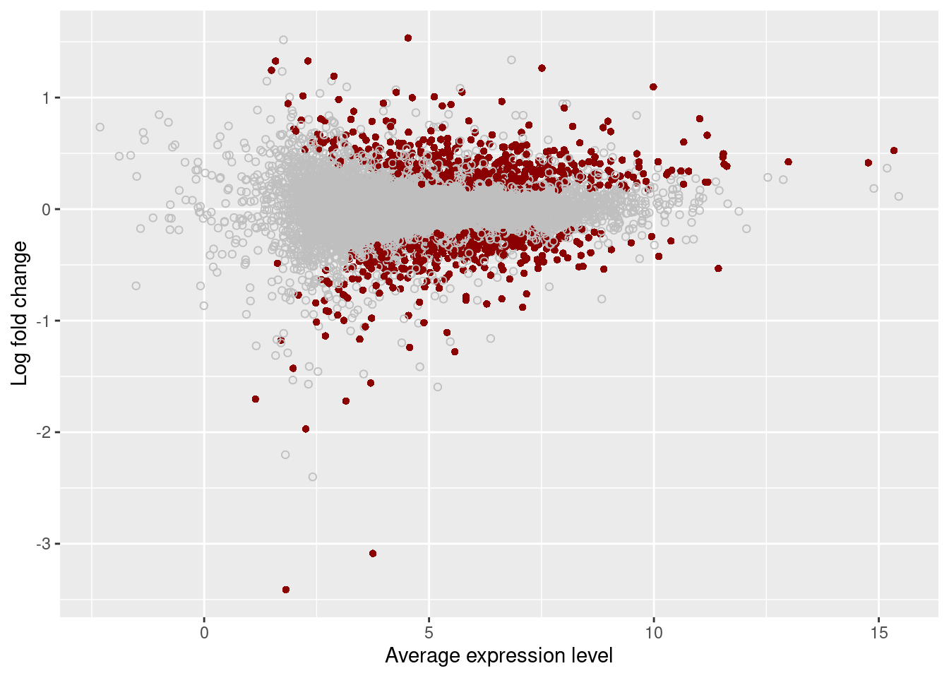
plot_volcano(results[["Unstrain"]], 0.05)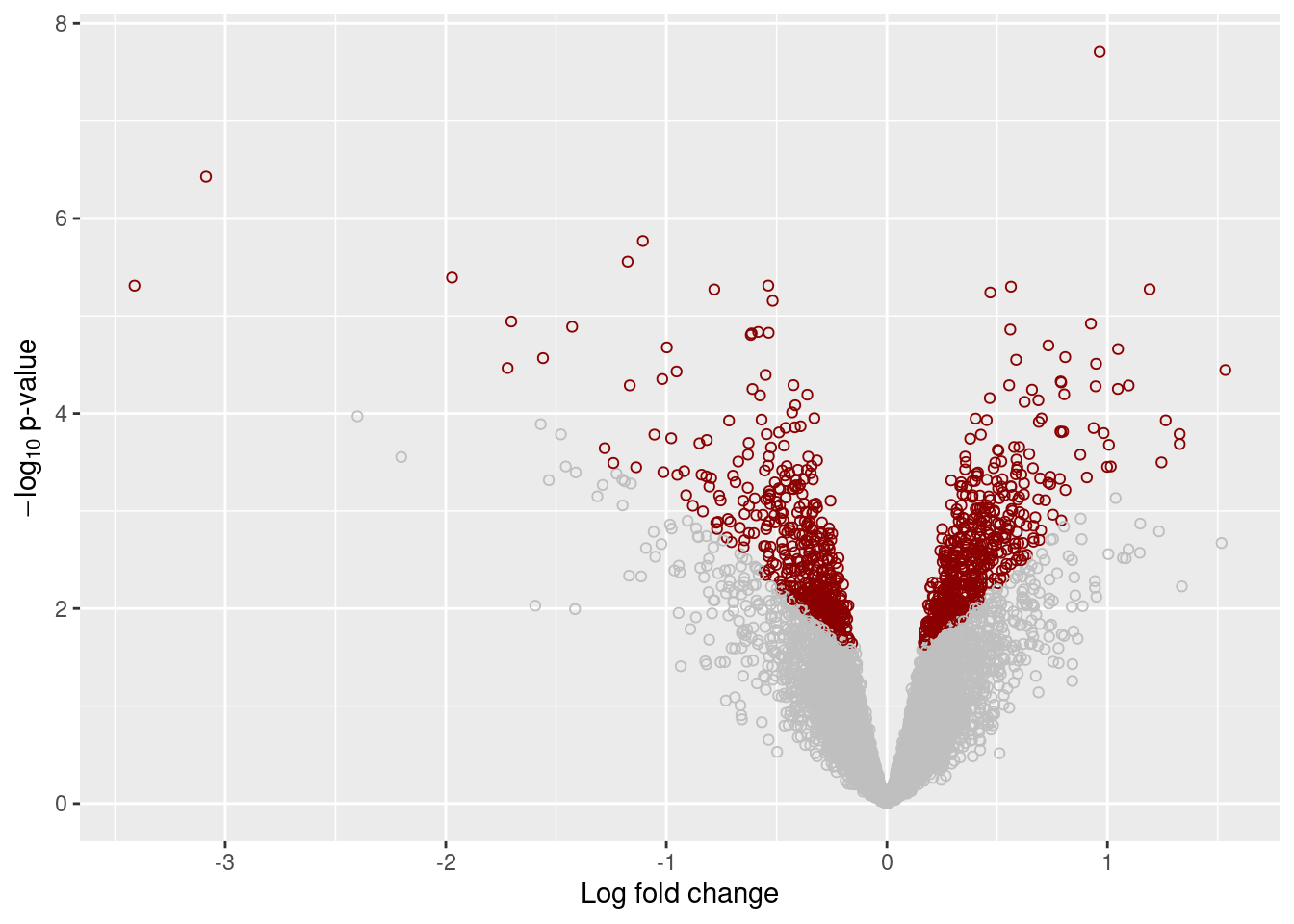
plot_pval_hist(results[["Unstrain"]], 0.05)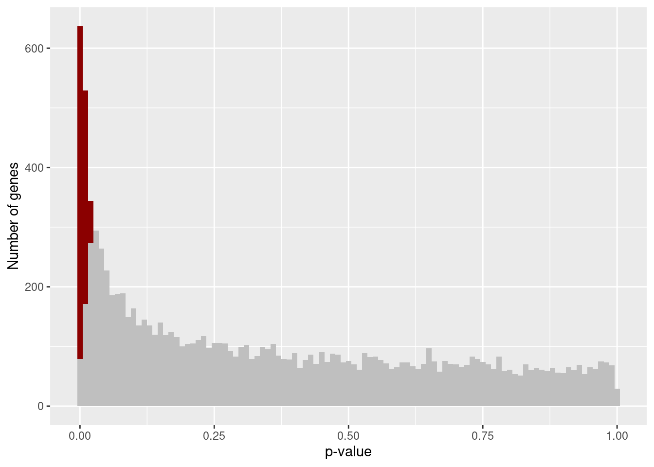
table(results[["Unstrain"]]$qvalue < 0.05)
FALSE TRUE
9499 987 significant_genes_05 <- row.names(results[["Unstrain"]])[results[["Unstrain"]]$qvalue < 0.05]
significant_symbols_05 <- gene_anno$external_gene_name[match(significant_genes_05, gene_anno$ensembl_gene_id)]
head(significant_symbols_05)[1] DVL1 MRPL20 MMP23B PEX10 CEP104 ACOT7
56858 Levels: A1BG A1BG-AS1 A1CF A2M A2M-AS1 A2ML1 A2ML1-AS1 ... ZZEF1significant_anno_05 <- gene_anno[match(significant_genes_05, gene_anno$ensembl_gene_id),]Gene ontology analysis with topGO
Use topGO for GO analysis. It accounts for the nested graph structure of GO terms to prune the number of GO categories tested (Alexa et al. 2006). Essentially, it decreases the redundancy of the results.
# k-s test making use of ranked based on p-values
genes <- results[["Unstrain"]]$qvalue
names(genes) <- rownames(results[["Unstrain"]])
selection <- function(allScore){ return(allScore < 0.05)} # function that returns TRUE/FALSE for p-values<0.05
allGO2genes <- annFUN.org(whichOnto="BP", feasibleGenes=NULL, mapping="org.Hs.eg.db", ID="ensembl")Loading required package: org.Hs.eg.dbGOdata <- new("topGOdata",
ontology="BP",
allGenes=genes,
annot=annFUN.GO2genes,
GO2genes=allGO2genes,
geneSel=selection,
nodeSize=10)
Building most specific GOs ..... ( 9780 GO terms found. )
Build GO DAG topology .......... ( 13861 GO terms and 32652 relations. )
Annotating nodes ............... ( 9204 genes annotated to the GO terms. )results.ks <- runTest(GOdata, algorithm="classic", statistic="ks")
-- Classic Algorithm --
the algorithm is scoring 5178 nontrivial nodes
parameters:
test statistic: ks
score order: increasinggoEnrichment <- GenTable(GOdata, KS=results.ks, orderBy="KS", topNodes=20)
goEnrichment <- goEnrichment %>%
mutate(KS = ifelse(grepl("<", KS), 1e-30, KS))
goEnrichment$KS <- as.numeric(goEnrichment$KS)
goEnrichment <- goEnrichment[goEnrichment$KS<0.05,]
goEnrichment <- goEnrichment[,c("GO.ID","Term","KS")]
goEnrichment$Term <- gsub(" [a-z]*\\.\\.\\.$", "", goEnrichment$Term)
goEnrichment$Term <- gsub("\\.\\.\\.$", "", goEnrichment$Term)
goEnrichment$Term <- paste(goEnrichment$GO.ID, goEnrichment$Term, sep=", ")
goEnrichment$Term <- factor(goEnrichment$Term, levels=rev(goEnrichment$Term))
goEnrichment$KS <- as.numeric(goEnrichment$KS)
ggplot(goEnrichment, aes(x=Term, y=-log10(KS))) +
stat_summary(geom = "bar", fun = mean, position = "dodge") +
xlab("Biological process") +
ylab("Enrichment") +
ggtitle("Title") +
scale_y_continuous(breaks = round(seq(0, max(-log10(goEnrichment$KS)), by = 2), 1)) +
theme_bw(base_size=24) +
theme(
legend.position='none',
legend.background=element_rect(),
plot.title=element_text(angle=0, size=24, face="bold", vjust=1),
axis.text.x=element_text(angle=0, size=18, face="bold", hjust=1.10),
axis.text.y=element_text(angle=0, size=18, face="bold", vjust=0.5),
axis.title=element_text(size=24, face="bold"),
legend.key=element_blank(), #removes the border
legend.key.size=unit(1, "cm"), #Sets overall area/size of the legend
legend.text=element_text(size=18), #Text size
title=element_text(size=18)) +
guides(colour=guide_legend(override.aes=list(size=2.5))) +
coord_flip()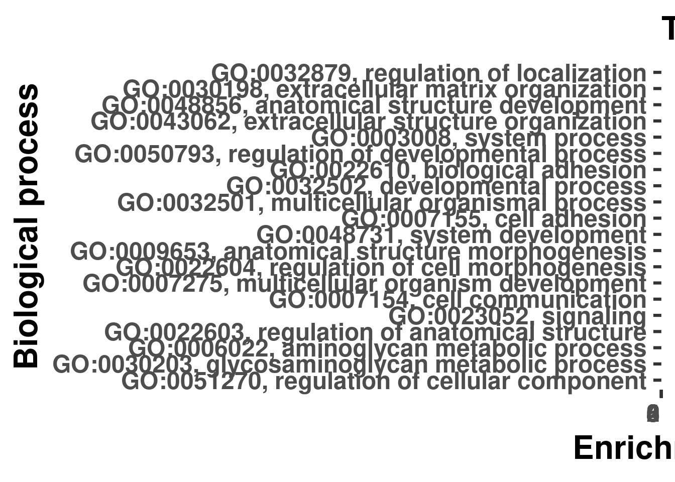
Additional analysis permuting samples:
From Ben Fair: “i have a suggestion for an analysis as a check that all your DE results (like the GO analysis, the enrichment for DE genes from published datasets) are robust… i’m not sure this is statistically perfect but its something that I think makes sense to try, for my own sanity: if you randomly reassign control and treatment labels and re-attampt DE testing, do all of those interesting results go away? the worry i am trying to address, is that you have some enrichment of DE genes in interesting GO categories for example, but is that just because you have more DE power for detecting highly expressed genes in this cell type (even if they are only modestly or not truly DE), and that is what drives the GO enrichment.”
#scramble treatment labels (x3) and store the DE genes (each time, randomly assign 9 samples to be strain)
permuted_results <- vector("list", 12)
for(time in 1:6){
#set up DE and scramble labels
anno <- pData(RUVsOut)
x <- paste0(anno$Individual, anno$treatment)
anno$LibraryPrepBatch <- factor(anno$LibraryPrepBatch, levels = c("1", "2"))
anno$Replicate <- factor(anno$Replicate, levels = c("1", "2", "3"))
strain_indices <- sample(nrow(anno), 9)
anno$treatment <- "Unstrain"
anno$treatment[strain_indices] <- "Strain"
design <- model.matrix(~treatment + Individual + W_1 + W_2 + RIN,
data = anno)
colnames(design) <- gsub("treatment", "", colnames(design))
permuted_results[[time]] <- anno
#perform DE
#TMM Normalization
y <- DGEList(filt_counts)
y <- calcNormFactors(y, method = "TMM")
#Voom for differential expression
v1 <- voom(y, design)
corfit1 <- duplicateCorrelation(v1, design, block = x)
corfit1$consensus.correlation
v2 <- voom(y, design, block = x, correlation = corfit1$consensus.correlation)
corfit2 <- duplicateCorrelation(v2, design, block = x)
corfit2$consensus.correlation
fit <- lmFit(v2, design, block = x,
correlation = corfit2$consensus.correlation)
fit <- eBayes(fit)
tests <- colnames(fit$coefficients)
results <- vector(length = length(tests), mode = "list")
names(results) <- tests
for (test in tests[c(1:7)]) {
# Extract limma results
results[[test]] <- get_results(fit, coef = test)
# Add mutliple testing correction with ASH
output_ash <- run_ash(fit, coef = test)$result
results[[test]] <- cbind(results[[test]], lfsr = output_ash$lfsr,
lfdr = output_ash$lfdr, qvalue = output_ash$qvalue,
svalue = output_ash$svalue)
}
#store results
permuted_results[[6+time]] <- results[["Unstrain"]]
}Warning in glmgam.fit(dx, dy, coef.start = start, tol = tol, maxit =
maxit, : Too much damping - convergence tolerance not achievable
Warning in glmgam.fit(dx, dy, coef.start = start, tol = tol, maxit =
maxit, : Too much damping - convergence tolerance not achievable
Warning in glmgam.fit(dx, dy, coef.start = start, tol = tol, maxit =
maxit, : Too much damping - convergence tolerance not achievable
Warning in glmgam.fit(dx, dy, coef.start = start, tol = tol, maxit =
maxit, : Too much damping - convergence tolerance not achievable
Warning in glmgam.fit(dx, dy, coef.start = start, tol = tol, maxit =
maxit, : Too much damping - convergence tolerance not achievable
Warning in glmgam.fit(dx, dy, coef.start = start, tol = tol, maxit =
maxit, : Too much damping - convergence tolerance not achievable
Warning in glmgam.fit(dx, dy, coef.start = start, tol = tol, maxit =
maxit, : Too much damping - convergence tolerance not achievable
Warning in glmgam.fit(dx, dy, coef.start = start, tol = tol, maxit =
maxit, : Too much damping - convergence tolerance not achievable
Warning in glmgam.fit(dx, dy, coef.start = start, tol = tol, maxit =
maxit, : Too much damping - convergence tolerance not achievable
Warning in glmgam.fit(dx, dy, coef.start = start, tol = tol, maxit =
maxit, : Too much damping - convergence tolerance not achievable#visualize what the permutations look like (what the scrambled labels look like)
for(time in 1:6){
print(permuted_results[[time]])
} Sample_ID Individual Sex Replicate treatment RIN
18855_3_S 18855_3_S NA18855 F 3 Unstrain 10.0
19160_3_S 19160_3_S NA19160 M 3 Strain 10.0
18856_3_U 18856_3_U NA18856 M 3 Strain 10.0
18856_1_U 18856_1_U NA18856 M 1 Unstrain 9.9
18855_2_S 18855_2_S NA18855 F 2 Unstrain 10.0
18856_2_S 18856_2_S NA18856 M 2 Strain 9.6
19160_3_U 19160_3_U NA19160 M 3 Strain 10.0
18855_2_U 18855_2_U NA18855 F 2 Unstrain 10.0
19160_2_S 19160_2_S NA19160 M 2 Unstrain 10.0
18855_1_S 18855_1_S NA18855 F 1 Unstrain 9.9
18856_1_S 18856_1_S NA18856 M 1 Unstrain 8.5
19160_1_S 19160_1_S NA19160 M 1 Strain 9.9
19160_2_U 19160_2_U NA19160 M 2 Strain 10.0
18855_1_U 18855_1_U NA18855 F 1 Strain 10.0
18856_3_S 18856_3_S NA18856 M 3 Strain 9.6
18856_2_U 18856_2_U NA18856 M 2 Strain 9.5
18855_3_U 18855_3_U NA18855 F 3 Unstrain 10.0
LibraryPrepBatch LibSize W_1 W_2
18855_3_S 2 15419569 0.541963415 -1.1181740
19160_3_S 2 15177653 0.376349314 -1.4100700
18856_3_U 2 13722909 0.857248982 -0.8808562
18856_1_U 1 18647599 1.113674153 -1.5466409
18855_2_S 1 18256163 0.733375747 -0.7617020
18856_2_S 1 16782764 -0.051863231 -1.3484210
19160_3_U 2 19839604 0.224499121 -1.5560509
18855_2_U 1 18618691 0.665015743 -0.9464050
19160_2_S 1 16622407 0.308745015 -1.5149287
18855_1_S 1 19712744 0.626769726 -1.5366695
18856_1_S 1 13571439 1.038716806 -1.2664724
19160_1_S 1 20979958 0.461484490 -2.0300296
19160_2_U 1 20924281 0.002654243 -1.9184820
18855_1_U 1 20146697 0.649711618 -1.4110342
18856_3_S 2 15807863 0.728747075 -0.9909086
18856_2_U 1 15142152 0.359175096 -1.0809905
18855_3_U 2 18157918 0.487681866 -1.2290497
Sample_ID Individual Sex Replicate treatment RIN
18855_3_S 18855_3_S NA18855 F 3 Strain 10.0
19160_3_S 19160_3_S NA19160 M 3 Unstrain 10.0
18856_3_U 18856_3_U NA18856 M 3 Strain 10.0
18856_1_U 18856_1_U NA18856 M 1 Unstrain 9.9
18855_2_S 18855_2_S NA18855 F 2 Strain 10.0
18856_2_S 18856_2_S NA18856 M 2 Strain 9.6
19160_3_U 19160_3_U NA19160 M 3 Unstrain 10.0
18855_2_U 18855_2_U NA18855 F 2 Strain 10.0
19160_2_S 19160_2_S NA19160 M 2 Strain 10.0
18855_1_S 18855_1_S NA18855 F 1 Unstrain 9.9
18856_1_S 18856_1_S NA18856 M 1 Strain 8.5
19160_1_S 19160_1_S NA19160 M 1 Unstrain 9.9
19160_2_U 19160_2_U NA19160 M 2 Unstrain 10.0
18855_1_U 18855_1_U NA18855 F 1 Unstrain 10.0
18856_3_S 18856_3_S NA18856 M 3 Unstrain 9.6
18856_2_U 18856_2_U NA18856 M 2 Strain 9.5
18855_3_U 18855_3_U NA18855 F 3 Strain 10.0
LibraryPrepBatch LibSize W_1 W_2
18855_3_S 2 15419569 0.541963415 -1.1181740
19160_3_S 2 15177653 0.376349314 -1.4100700
18856_3_U 2 13722909 0.857248982 -0.8808562
18856_1_U 1 18647599 1.113674153 -1.5466409
18855_2_S 1 18256163 0.733375747 -0.7617020
18856_2_S 1 16782764 -0.051863231 -1.3484210
19160_3_U 2 19839604 0.224499121 -1.5560509
18855_2_U 1 18618691 0.665015743 -0.9464050
19160_2_S 1 16622407 0.308745015 -1.5149287
18855_1_S 1 19712744 0.626769726 -1.5366695
18856_1_S 1 13571439 1.038716806 -1.2664724
19160_1_S 1 20979958 0.461484490 -2.0300296
19160_2_U 1 20924281 0.002654243 -1.9184820
18855_1_U 1 20146697 0.649711618 -1.4110342
18856_3_S 2 15807863 0.728747075 -0.9909086
18856_2_U 1 15142152 0.359175096 -1.0809905
18855_3_U 2 18157918 0.487681866 -1.2290497
Sample_ID Individual Sex Replicate treatment RIN
18855_3_S 18855_3_S NA18855 F 3 Unstrain 10.0
19160_3_S 19160_3_S NA19160 M 3 Unstrain 10.0
18856_3_U 18856_3_U NA18856 M 3 Strain 10.0
18856_1_U 18856_1_U NA18856 M 1 Unstrain 9.9
18855_2_S 18855_2_S NA18855 F 2 Strain 10.0
18856_2_S 18856_2_S NA18856 M 2 Unstrain 9.6
19160_3_U 19160_3_U NA19160 M 3 Strain 10.0
18855_2_U 18855_2_U NA18855 F 2 Strain 10.0
19160_2_S 19160_2_S NA19160 M 2 Strain 10.0
18855_1_S 18855_1_S NA18855 F 1 Unstrain 9.9
18856_1_S 18856_1_S NA18856 M 1 Unstrain 8.5
19160_1_S 19160_1_S NA19160 M 1 Strain 9.9
19160_2_U 19160_2_U NA19160 M 2 Strain 10.0
18855_1_U 18855_1_U NA18855 F 1 Unstrain 10.0
18856_3_S 18856_3_S NA18856 M 3 Strain 9.6
18856_2_U 18856_2_U NA18856 M 2 Unstrain 9.5
18855_3_U 18855_3_U NA18855 F 3 Strain 10.0
LibraryPrepBatch LibSize W_1 W_2
18855_3_S 2 15419569 0.541963415 -1.1181740
19160_3_S 2 15177653 0.376349314 -1.4100700
18856_3_U 2 13722909 0.857248982 -0.8808562
18856_1_U 1 18647599 1.113674153 -1.5466409
18855_2_S 1 18256163 0.733375747 -0.7617020
18856_2_S 1 16782764 -0.051863231 -1.3484210
19160_3_U 2 19839604 0.224499121 -1.5560509
18855_2_U 1 18618691 0.665015743 -0.9464050
19160_2_S 1 16622407 0.308745015 -1.5149287
18855_1_S 1 19712744 0.626769726 -1.5366695
18856_1_S 1 13571439 1.038716806 -1.2664724
19160_1_S 1 20979958 0.461484490 -2.0300296
19160_2_U 1 20924281 0.002654243 -1.9184820
18855_1_U 1 20146697 0.649711618 -1.4110342
18856_3_S 2 15807863 0.728747075 -0.9909086
18856_2_U 1 15142152 0.359175096 -1.0809905
18855_3_U 2 18157918 0.487681866 -1.2290497
Sample_ID Individual Sex Replicate treatment RIN
18855_3_S 18855_3_S NA18855 F 3 Unstrain 10.0
19160_3_S 19160_3_S NA19160 M 3 Strain 10.0
18856_3_U 18856_3_U NA18856 M 3 Unstrain 10.0
18856_1_U 18856_1_U NA18856 M 1 Strain 9.9
18855_2_S 18855_2_S NA18855 F 2 Unstrain 10.0
18856_2_S 18856_2_S NA18856 M 2 Strain 9.6
19160_3_U 19160_3_U NA19160 M 3 Strain 10.0
18855_2_U 18855_2_U NA18855 F 2 Unstrain 10.0
19160_2_S 19160_2_S NA19160 M 2 Strain 10.0
18855_1_S 18855_1_S NA18855 F 1 Unstrain 9.9
18856_1_S 18856_1_S NA18856 M 1 Strain 8.5
19160_1_S 19160_1_S NA19160 M 1 Strain 9.9
19160_2_U 19160_2_U NA19160 M 2 Strain 10.0
18855_1_U 18855_1_U NA18855 F 1 Unstrain 10.0
18856_3_S 18856_3_S NA18856 M 3 Unstrain 9.6
18856_2_U 18856_2_U NA18856 M 2 Strain 9.5
18855_3_U 18855_3_U NA18855 F 3 Unstrain 10.0
LibraryPrepBatch LibSize W_1 W_2
18855_3_S 2 15419569 0.541963415 -1.1181740
19160_3_S 2 15177653 0.376349314 -1.4100700
18856_3_U 2 13722909 0.857248982 -0.8808562
18856_1_U 1 18647599 1.113674153 -1.5466409
18855_2_S 1 18256163 0.733375747 -0.7617020
18856_2_S 1 16782764 -0.051863231 -1.3484210
19160_3_U 2 19839604 0.224499121 -1.5560509
18855_2_U 1 18618691 0.665015743 -0.9464050
19160_2_S 1 16622407 0.308745015 -1.5149287
18855_1_S 1 19712744 0.626769726 -1.5366695
18856_1_S 1 13571439 1.038716806 -1.2664724
19160_1_S 1 20979958 0.461484490 -2.0300296
19160_2_U 1 20924281 0.002654243 -1.9184820
18855_1_U 1 20146697 0.649711618 -1.4110342
18856_3_S 2 15807863 0.728747075 -0.9909086
18856_2_U 1 15142152 0.359175096 -1.0809905
18855_3_U 2 18157918 0.487681866 -1.2290497
Sample_ID Individual Sex Replicate treatment RIN
18855_3_S 18855_3_S NA18855 F 3 Unstrain 10.0
19160_3_S 19160_3_S NA19160 M 3 Unstrain 10.0
18856_3_U 18856_3_U NA18856 M 3 Strain 10.0
18856_1_U 18856_1_U NA18856 M 1 Strain 9.9
18855_2_S 18855_2_S NA18855 F 2 Unstrain 10.0
18856_2_S 18856_2_S NA18856 M 2 Strain 9.6
19160_3_U 19160_3_U NA19160 M 3 Unstrain 10.0
18855_2_U 18855_2_U NA18855 F 2 Strain 10.0
19160_2_S 19160_2_S NA19160 M 2 Strain 10.0
18855_1_S 18855_1_S NA18855 F 1 Strain 9.9
18856_1_S 18856_1_S NA18856 M 1 Strain 8.5
19160_1_S 19160_1_S NA19160 M 1 Strain 9.9
19160_2_U 19160_2_U NA19160 M 2 Unstrain 10.0
18855_1_U 18855_1_U NA18855 F 1 Unstrain 10.0
18856_3_S 18856_3_S NA18856 M 3 Unstrain 9.6
18856_2_U 18856_2_U NA18856 M 2 Unstrain 9.5
18855_3_U 18855_3_U NA18855 F 3 Strain 10.0
LibraryPrepBatch LibSize W_1 W_2
18855_3_S 2 15419569 0.541963415 -1.1181740
19160_3_S 2 15177653 0.376349314 -1.4100700
18856_3_U 2 13722909 0.857248982 -0.8808562
18856_1_U 1 18647599 1.113674153 -1.5466409
18855_2_S 1 18256163 0.733375747 -0.7617020
18856_2_S 1 16782764 -0.051863231 -1.3484210
19160_3_U 2 19839604 0.224499121 -1.5560509
18855_2_U 1 18618691 0.665015743 -0.9464050
19160_2_S 1 16622407 0.308745015 -1.5149287
18855_1_S 1 19712744 0.626769726 -1.5366695
18856_1_S 1 13571439 1.038716806 -1.2664724
19160_1_S 1 20979958 0.461484490 -2.0300296
19160_2_U 1 20924281 0.002654243 -1.9184820
18855_1_U 1 20146697 0.649711618 -1.4110342
18856_3_S 2 15807863 0.728747075 -0.9909086
18856_2_U 1 15142152 0.359175096 -1.0809905
18855_3_U 2 18157918 0.487681866 -1.2290497
Sample_ID Individual Sex Replicate treatment RIN
18855_3_S 18855_3_S NA18855 F 3 Unstrain 10.0
19160_3_S 19160_3_S NA19160 M 3 Strain 10.0
18856_3_U 18856_3_U NA18856 M 3 Strain 10.0
18856_1_U 18856_1_U NA18856 M 1 Unstrain 9.9
18855_2_S 18855_2_S NA18855 F 2 Unstrain 10.0
18856_2_S 18856_2_S NA18856 M 2 Unstrain 9.6
19160_3_U 19160_3_U NA19160 M 3 Unstrain 10.0
18855_2_U 18855_2_U NA18855 F 2 Unstrain 10.0
19160_2_S 19160_2_S NA19160 M 2 Strain 10.0
18855_1_S 18855_1_S NA18855 F 1 Unstrain 9.9
18856_1_S 18856_1_S NA18856 M 1 Strain 8.5
19160_1_S 19160_1_S NA19160 M 1 Strain 9.9
19160_2_U 19160_2_U NA19160 M 2 Strain 10.0
18855_1_U 18855_1_U NA18855 F 1 Strain 10.0
18856_3_S 18856_3_S NA18856 M 3 Strain 9.6
18856_2_U 18856_2_U NA18856 M 2 Unstrain 9.5
18855_3_U 18855_3_U NA18855 F 3 Strain 10.0
LibraryPrepBatch LibSize W_1 W_2
18855_3_S 2 15419569 0.541963415 -1.1181740
19160_3_S 2 15177653 0.376349314 -1.4100700
18856_3_U 2 13722909 0.857248982 -0.8808562
18856_1_U 1 18647599 1.113674153 -1.5466409
18855_2_S 1 18256163 0.733375747 -0.7617020
18856_2_S 1 16782764 -0.051863231 -1.3484210
19160_3_U 2 19839604 0.224499121 -1.5560509
18855_2_U 1 18618691 0.665015743 -0.9464050
19160_2_S 1 16622407 0.308745015 -1.5149287
18855_1_S 1 19712744 0.626769726 -1.5366695
18856_1_S 1 13571439 1.038716806 -1.2664724
19160_1_S 1 20979958 0.461484490 -2.0300296
19160_2_U 1 20924281 0.002654243 -1.9184820
18855_1_U 1 20146697 0.649711618 -1.4110342
18856_3_S 2 15807863 0.728747075 -0.9909086
18856_2_U 1 15142152 0.359175096 -1.0809905
18855_3_U 2 18157918 0.487681866 -1.2290497for (permutation in 7:12){
results <- permuted_results[[permutation]]
# k-s test making use of ranked based on p-values
genes <- results$qvalue
names(genes) <- rownames(results)
selection <- function(allScore){ return(allScore < 0.05)} # function that returns TRUE/FALSE for p-values<0.05
allGO2genes <- annFUN.org(whichOnto="BP", feasibleGenes=NULL, mapping="org.Hs.eg.db", ID="ensembl")
GOdata <- new("topGOdata",
  ontology="BP",
  allGenes=genes,
  annot=annFUN.GO2genes,
  GO2genes=allGO2genes,
  geneSel=selection,
  nodeSize=10)
results.ks <- runTest(GOdata, algorithm="classic", statistic="ks")
goEnrichment <- GenTable(GOdata, KS=results.ks, orderBy="KS", topNodes=20)
goEnrichment <- goEnrichment %>%
mutate(KS = ifelse(grepl("<", KS), 1e-30, KS))
goEnrichment$KS <- as.numeric(goEnrichment$KS)
goEnrichment <- goEnrichment[goEnrichment$KS<0.05,]
goEnrichment <- goEnrichment[,c("GO.ID","Term","KS")]
goEnrichment$Term <- gsub(" [a-z]*\\.\\.\\.$", "", goEnrichment$Term)
goEnrichment$Term <- gsub("\\.\\.\\.$", "", goEnrichment$Term)
goEnrichment$Term <- paste(goEnrichment$GO.ID, goEnrichment$Term, sep=", ")
goEnrichment$Term <- factor(goEnrichment$Term, levels=rev(goEnrichment$Term))
goEnrichment$KS <- as.numeric(goEnrichment$KS)
plot <- ggplot(goEnrichment, aes(x=Term, y=-log10(KS))) +
stat_summary(geom = "bar", fun = mean, position = "dodge") +
xlab("Biological process") +
ylab("Enrichment") +
ggtitle("Title") +
scale_y_continuous(breaks = round(seq(0, max(-log10(goEnrichment$KS)), by = 2), 1)) +
theme_bw(base_size=24) +
theme(
legend.position='none',
legend.background=element_rect(),
plot.title=element_text(angle=0, size=24, face="bold", vjust=1),
axis.text.x=element_text(angle=0, size=18, face="bold", hjust=1.10),
axis.text.y=element_text(angle=0, size=18, face="bold", vjust=0.5),
axis.title=element_text(size=24, face="bold"),
legend.key=element_blank(), #removes the border
legend.key.size=unit(1, "cm"), #Sets overall area/size of the legend
legend.text=element_text(size=18), #Text size
title=element_text(size=18)) +
guides(colour=guide_legend(override.aes=list(size=2.5))) +
coord_flip()
print(plot)
}
Building most specific GOs ..... ( 9780 GO terms found. )
Build GO DAG topology .......... ( 13861 GO terms and 32652 relations. )
Annotating nodes ............... ( 9204 genes annotated to the GO terms. )
             -- Classic Algorithm --

         the algorithm is scoring 5178 nontrivial nodes
         parameters:
             test statistic: ks
             score order: increasing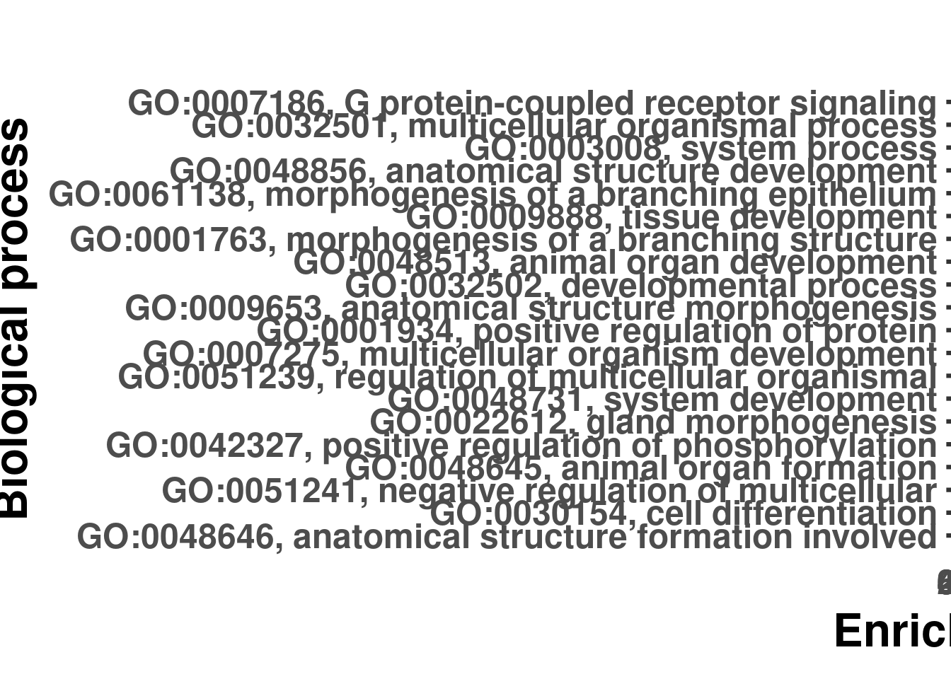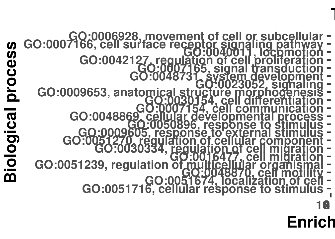
for (permutation in 7:12){
results <- permuted_results[[permutation]]
# k-s test making use of ranked based on p-values
genes <- results$qvalue
names(genes) <- rownames(results)
selection <- function(allScore){ return(allScore < 0.05)} # function that returns TRUE/FALSE for p-values<0.05
allGO2genes <- annFUN.org(whichOnto="BP", feasibleGenes=NULL, mapping="org.Hs.eg.db", ID="ensembl")
GOdata <- new("topGOdata",
ontology="BP",
allGenes=genes,
annot=annFUN.GO2genes,
GO2genes=allGO2genes,
geneSel=selection,
nodeSize=10)
results.ks <- runTest(GOdata, algorithm="classic", statistic="ks")
goEnrichment <- GenTable(GOdata, KS=results.ks, orderBy="KS", topNodes=20)
goEnrichment <- goEnrichment %>%
mutate(KS = ifelse(grepl("<", KS), 1e-30, KS))
goEnrichment$KS <- as.numeric(goEnrichment$KS)
goEnrichment <- goEnrichment[goEnrichment$KS<0.05,]
goEnrichment <- goEnrichment[,c("GO.ID","Term","KS")]
goEnrichment$Term <- gsub(" [a-z]*\\.\\.\\.$", "", goEnrichment$Term)
goEnrichment$Term <- gsub("\\.\\.\\.$", "", goEnrichment$Term)
goEnrichment$Term <- paste(goEnrichment$GO.ID, goEnrichment$Term, sep=", ")
goEnrichment$Term <- factor(goEnrichment$Term, levels=rev(goEnrichment$Term))
goEnrichment$KS <- as.numeric(goEnrichment$KS)
print(goEnrichment$Term)
}
Building most specific GOs ..... ( 9780 GO terms found. )
Build GO DAG topology .......... ( 13861 GO terms and 32652 relations. )
Annotating nodes ............... ( 9204 genes annotated to the GO terms. )
             -- Classic Algorithm --

         the algorithm is scoring 5178 nontrivial nodes
         parameters:
             test statistic: ks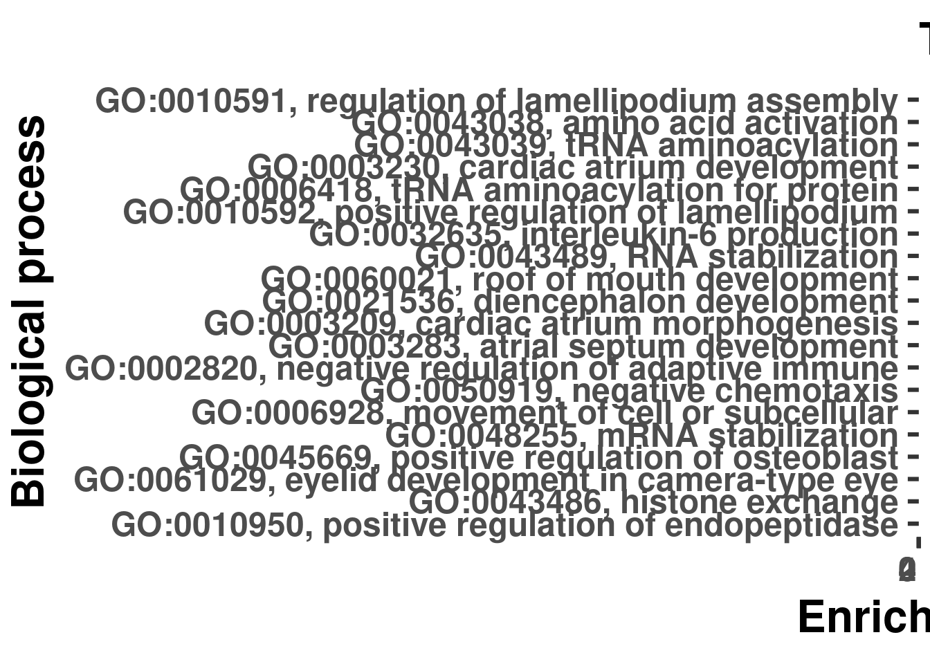
score order: increasing [1] GO:0010591, regulation of lamellipodium assembly
[2] GO:0043038, amino acid activation
[3] GO:0043039, tRNA aminoacylation
[4] GO:0003230, cardiac atrium development
[5] GO:0006418, tRNA aminoacylation for protein
[6] GO:0010592, positive regulation of lamellipodium
[7] GO:0032635, interleukin-6 production
[8] GO:0043489, RNA stabilization
[9] GO:0060021, roof of mouth development
[10] GO:0021536, diencephalon development
[11] GO:0003209, cardiac atrium morphogenesis
[12] GO:0003283, atrial septum development
[13] GO:0002820, negative regulation of adaptive immune
[14] GO:0050919, negative chemotaxis
[15] GO:0006928, movement of cell or subcellular
[16] GO:0048255, mRNA stabilization
[17] GO:0045669, positive regulation of osteoblast
[18] GO:0061029, eyelid development in camera-type eye
[19] GO:0043486, histone exchange
[20] GO:0010950, positive regulation of endopeptidase
20 Levels: GO:0010950, positive regulation of endopeptidase ...
Building most specific GOs ..... ( 9780 GO terms found. )
Build GO DAG topology .......... ( 13861 GO terms and 32652 relations. )
Annotating nodes ............... ( 9204 genes annotated to the GO terms. )
             -- Classic Algorithm --

         the algorithm is scoring 5178 nontrivial nodes
         parameters:
             test statistic: ks
             score order: increasing
[1] GO:0007186, G protein-coupled receptor signaling
[2] GO:0032501, multicellular organismal process
[3] GO:0003008, system process
[4] GO:0048856, anatomical structure development
[5] GO:0061138, morphogenesis of a branching epithelium
[6] GO:0009888, tissue development
[7] GO:0001763, morphogenesis of a branching structure
[8] GO:0048513, animal organ development
[9] GO:0032502, developmental process
[10] GO:0009653, anatomical structure morphogenesis
[11] GO:0001934, positive regulation of protein
[12] GO:0007275, multicellular organism development
[13] GO:0051239, regulation of multicellular organismal
[14] GO:0048731, system development
[15] GO:0022612, gland morphogenesis
[16] GO:0042327, positive regulation of phosphorylation
[17] GO:0048645, animal organ formation
[18] GO:0051241, negative regulation of multicellular
[19] GO:0030154, cell differentiation
[20] GO:0048646, anatomical structure formation involved
20 Levels: GO:0048646, anatomical structure formation involved ...
Building most specific GOs ..... ( 9780 GO terms found. )
Build GO DAG topology .......... ( 13861 GO terms and 32652 relations. )
Annotating nodes ............... ( 9204 genes annotated to the GO terms. )
             -- Classic Algorithm --

         the algorithm is scoring 5178 nontrivial nodes
         parameters:
             test statistic: ks
             score order: increasing
[1] GO:0010591, regulation of lamellipodium assembly
[2] GO:0043038, amino acid activation
[3] GO:0043039, tRNA aminoacylation
[4] GO:0003230, cardiac atrium development
[5] GO:0006418, tRNA aminoacylation for protein
[6] GO:0010592, positive regulation of lamellipodium
[7] GO:0032635, interleukin-6 production
[8] GO:0043489, RNA stabilization
[9] GO:0060021, roof of mouth development
[10] GO:0021536, diencephalon development
[11] GO:0003209, cardiac atrium morphogenesis
[12] GO:0003283, atrial septum development
[13] GO:0002820, negative regulation of adaptive immune
[14] GO:0050919, negative chemotaxis
[15] GO:0006928, movement of cell or subcellular
[16] GO:0048255, mRNA stabilization
[17] GO:0045669, positive regulation of osteoblast
[18] GO:0061029, eyelid development in camera-type eye
[19] GO:0043486, histone exchange
[20] GO:0010950, positive regulation of endopeptidase
20 Levels: GO:0010950, positive regulation of endopeptidase ...
Building most specific GOs ..... ( 9780 GO terms found. )
Build GO DAG topology .......... ( 13861 GO terms and 32652 relations. )
Annotating nodes ............... ( 9204 genes annotated to the GO terms. )
             -- Classic Algorithm --

         the algorithm is scoring 5178 nontrivial nodes
         parameters:
             test statistic: ks
             score order: increasing
[1] GO:0006928, movement of cell or subcellular
[2] GO:0007166, cell surface receptor signaling pathway
[3] GO:0040011, locomotion
[4] GO:0042127, regulation of cell proliferation
[5] GO:0007165, signal transduction
[6] GO:0048731, system development
[7] GO:0023052, signaling
[8] GO:0009653, anatomical structure morphogenesis
[9] GO:0030154, cell differentiation
[10] GO:0007154, cell communication
[11] GO:0048869, cellular developmental process
[12] GO:0050896, response to stimulus
[13] GO:0009605, response to external stimulus
[14] GO:0051270, regulation of cellular component
[15] GO:0030334, regulation of cell migration
[16] GO:0016477, cell migration
[17] GO:0051239, regulation of multicellular organismal
[18] GO:0048870, cell motility
[19] GO:0051674, localization of cell
[20] GO:0051716, cellular response to stimulus
20 Levels: GO:0051716, cellular response to stimulus ...
Building most specific GOs ..... ( 9780 GO terms found. )
Build GO DAG topology .......... ( 13861 GO terms and 32652 relations. )
Annotating nodes ............... ( 9204 genes annotated to the GO terms. )
             -- Classic Algorithm --

         the algorithm is scoring 5178 nontrivial nodes
         parameters:
             test statistic: ks
             score order: increasing
[1] GO:0010591, regulation of lamellipodium assembly
[2] GO:0043038, amino acid activation
[3] GO:0043039, tRNA aminoacylation
[4] GO:0003230, cardiac atrium development
[5] GO:0006418, tRNA aminoacylation for protein
[6] GO:0010592, positive regulation of lamellipodium
[7] GO:0032635, interleukin-6 production
[8] GO:0043489, RNA stabilization
[9] GO:0060021, roof of mouth development
[10] GO:0021536, diencephalon development
[11] GO:0003209, cardiac atrium morphogenesis
[12] GO:0003283, atrial septum development
[13] GO:0002820, negative regulation of adaptive immune
[14] GO:0050919, negative chemotaxis
[15] GO:0006928, movement of cell or subcellular
[16] GO:0048255, mRNA stabilization
[17] GO:0045669, positive regulation of osteoblast
[18] GO:0061029, eyelid development in camera-type eye
[19] GO:0043486, histone exchange
[20] GO:0010950, positive regulation of endopeptidase
20 Levels: GO:0010950, positive regulation of endopeptidase ...
Building most specific GOs ..... ( 9780 GO terms found. )
Build GO DAG topology .......... ( 13861 GO terms and 32652 relations. )
Annotating nodes ............... ( 9204 genes annotated to the GO terms. )
             -- Classic Algorithm --

         the algorithm is scoring 5178 nontrivial nodes
         parameters:
             test statistic: ks
             score order: increasing
[1] GO:0010591, regulation of lamellipodium assembly
[2] GO:0043038, amino acid activation
[3] GO:0043039, tRNA aminoacylation
[4] GO:0003230, cardiac atrium development
[5] GO:0006418, tRNA aminoacylation for protein
[6] GO:0010592, positive regulation of lamellipodium
[7] GO:0032635, interleukin-6 production
[8] GO:0043489, RNA stabilization
[9] GO:0060021, roof of mouth development
[10] GO:0021536, diencephalon development
[11] GO:0003209, cardiac atrium morphogenesis
[12] GO:0003283, atrial septum development
[13] GO:0002820, negative regulation of adaptive immune
[14] GO:0050919, negative chemotaxis
[15] GO:0006928, movement of cell or subcellular
[16] GO:0048255, mRNA stabilization
[17] GO:0045669, positive regulation of osteoblast
[18] GO:0061029, eyelid development in camera-type eye
[19] GO:0043486, histone exchange
[20] GO:0010950, positive regulation of endopeptidase
20 Levels: GO:0010950, positive regulation of endopeptidase ...Enrichment Function
Use fisher’s exact test to compute significant enrichment.
enrich <- function(genes_of_interest, DEgenes, backgroundgenes){
     #fill contingency table
     DE_interest <- length(intersect(genes_of_interest, DEgenes))
     background_interest <- length(intersect(genes_of_interest, backgroundgenes))
     DE_non_interest <- length(DEgenes) - DE_interest
     background_non_interest <- length(backgroundgenes) - background_interest
     contingency_table <- matrix(c(DE_interest, background_interest, DE_non_interest, background_non_interest), nrow = 2, ncol = 2, byrow = TRUE)

     #perform test
     print(contingency_table)
     return(fisher.test(contingency_table, alternative="greater"))
}


enrich(fungenomic, DE_genes_ensg, other_genes_ensg)
[,1] [,2]
[1,] 0 0
[2,] 0 0
    Fisher's Exact Test for Count Data

data:  contingency_table
p-value = 1
alternative hypothesis: true odds ratio is greater than 1
95 percent confidence interval:
   0 Inf
sample estimates:
odds ratio
         0
enrich(cross_omic, DE_genes_ensg, other_genes_ensg) [,1] [,2]
[1,] 0 0
[2,] 0 0
    Fisher's Exact Test for Count Data

data:  contingency_table
p-value = 1
alternative hypothesis: true odds ratio is greater than 1
95 percent confidence interval:
   0 Inf
sample estimates:
odds ratio
         0
Look at enrichments from permuted DE analysis (scrambled strain labels to make sure the FET results aren’t just because some genes are more likely to be detected as DE in these cells)
threshold <- 0.05
for(permutation in 7:12){
     print(permutation)
     DE_results <- permuted_results[[permutation]]
     DE_genes_ensg <- rownames(DE_results)[DE_results$qvalue < threshold]
     DE_genes <- gene_anno$external_gene_name[match(DE_genes_ensg, gene_anno$ensembl_gene_id)]
     other_genes_ensg <- rownames(DE_results)[DE_results$qvalue >= threshold]
     other_genes <- gene_anno$external_gene_name[match(other_genes_ensg, gene_anno$ensembl_gene_id)]

     print(enrich(fungenomic, DE_genes_ensg, other_genes_ensg))
     print(enrich(cross_omic, DE_genes_ensg, other_genes_ensg))
}
[1] 7
[,1] [,2]
[1,] 0 342
[2,] 0 10144
Fisher's Exact Test for Count Data
data: contingency_table
p-value = 1
alternative hypothesis: true odds ratio is greater than 1
95 percent confidence interval:
0 Inf
sample estimates:
odds ratio
0
[,1] [,2]
[1,] 0 338
[2,] 0 10148
Fisher's Exact Test for Count Data
data: contingency_table
p-value = 1
alternative hypothesis: true odds ratio is greater than 1
95 percent confidence interval:
0 Inf
sample estimates:
odds ratio
0
[1] 8
[,1] [,2]
[1,] 0 342
[2,] 0 10144
Fisher's Exact Test for Count Data
data: contingency_table
p-value = 1
alternative hypothesis: true odds ratio is greater than 1
95 percent confidence interval:
0 Inf
sample estimates:
odds ratio
0
[,1] [,2]
[1,] 0 338
[2,] 0 10148
Fisher's Exact Test for Count Data
data: contingency_table
p-value = 1
alternative hypothesis: true odds ratio is greater than 1
95 percent confidence interval:
0 Inf
sample estimates:
odds ratio
0
[1] 9
[,1] [,2]
[1,] 0 342
[2,] 0 10144
Fisher's Exact Test for Count Data
data: contingency_table
p-value = 1
alternative hypothesis: true odds ratio is greater than 1
95 percent confidence interval:
0 Inf
sample estimates:
odds ratio
0
[,1] [,2]
[1,] 0 338
[2,] 0 10148
Fisher's Exact Test for Count Data
data: contingency_table
p-value = 1
alternative hypothesis: true odds ratio is greater than 1
95 percent confidence interval:
0 Inf
sample estimates:
odds ratio
0
[1] 10
[,1] [,2]
[1,] 0 342
[2,] 7 10137
Fisher's Exact Test for Count Data
data: contingency_table
p-value = 1
alternative hypothesis: true odds ratio is greater than 1
95 percent confidence interval:
0 Inf
sample estimates:
odds ratio
0
[,1] [,2]
[1,] 0 338
[2,] 7 10141
Fisher's Exact Test for Count Data
data: contingency_table
p-value = 1
alternative hypothesis: true odds ratio is greater than 1
95 percent confidence interval:
0 Inf
sample estimates:
odds ratio
0
[1] 11
[,1] [,2]
[1,] 0 342
[2,] 0 10144
Fisher's Exact Test for Count Data
data: contingency_table
p-value = 1
alternative hypothesis: true odds ratio is greater than 1
95 percent confidence interval:
0 Inf
sample estimates:
odds ratio
0
[,1] [,2]
[1,] 0 338
[2,] 0 10148
Fisher's Exact Test for Count Data
data: contingency_table
p-value = 1
alternative hypothesis: true odds ratio is greater than 1
95 percent confidence interval:
0 Inf
sample estimates:
odds ratio
0
[1] 12
[,1] [,2]
[1,] 0 342
[2,] 0 10144
Fisher's Exact Test for Count Data
data: contingency_table
p-value = 1
alternative hypothesis: true odds ratio is greater than 1
95 percent confidence interval:
0 Inf
sample estimates:
odds ratio
0
[,1] [,2]
[1,] 0 338
[2,] 0 10148
Fisher's Exact Test for Count Data
data: contingency_table
p-value = 1
alternative hypothesis: true odds ratio is greater than 1
95 percent confidence interval:
0 Inf
sample estimates:
odds ratio
0
sessionInfo()R version 3.6.1 (2019-07-05)
Platform: x86_64-pc-linux-gnu (64-bit)
Running under: Scientific Linux 7.4 (Nitrogen)
Matrix products: default
BLAS/LAPACK: /software/openblas-0.2.19-el7-x86_64/lib/libopenblas_haswellp-r0.2.19.so
locale:
[1] LC_CTYPE=en_US.UTF-8 LC_NUMERIC=C
[3] LC_TIME=en_US.UTF-8 LC_COLLATE=en_US.UTF-8
[5] LC_MONETARY=en_US.UTF-8 LC_MESSAGES=en_US.UTF-8
[7] LC_PAPER=en_US.UTF-8 LC_NAME=C
[9] LC_ADDRESS=C LC_TELEPHONE=C
[11] LC_MEASUREMENT=en_US.UTF-8 LC_IDENTIFICATION=C
attached base packages:
[1] stats4 parallel stats graphics grDevices utils datasets
[8] methods base
other attached packages:
[1] org.Hs.eg.db_3.8.2 topGO_2.36.0
[3] SparseM_1.78 GO.db_3.8.2
[5] AnnotationDbi_1.46.0 graph_1.62.0
[7] RUVSeq_1.18.0 EDASeq_2.18.0
[9] ShortRead_1.42.0 GenomicAlignments_1.20.1
[11] SummarizedExperiment_1.14.1 DelayedArray_0.10.0
[13] matrixStats_0.57.0 Rsamtools_2.0.0
[15] GenomicRanges_1.36.1 GenomeInfoDb_1.20.0
[17] Biostrings_2.52.0 XVector_0.24.0
[19] IRanges_2.18.3 S4Vectors_0.22.1
[21] BiocParallel_1.18.1 Biobase_2.44.0
[23] BiocGenerics_0.30.0 ggplot2_3.3.3
[25] ashr_2.2-47 tidyr_1.1.2
[27] edgeR_3.26.5 dplyr_1.0.2
[29] plyr_1.8.6 limma_3.40.6
loaded via a namespace (and not attached):
[1] bitops_1.0-6 fs_1.3.1 bit64_0.9-7
[4] httr_1.4.2 progress_1.2.2 RColorBrewer_1.1-2
[7] rprojroot_2.0.2 tools_3.6.1 R6_2.5.0
[10] irlba_2.3.3 DBI_1.1.0 colorspace_2.0-0
[13] withr_2.3.0 prettyunits_1.1.1 tidyselect_1.1.0
[16] bit_4.0.4 compiler_3.6.1 git2r_0.26.1
[19] labeling_0.4.2 rtracklayer_1.44.0 scales_1.1.1
[22] SQUAREM_2020.4 genefilter_1.66.0 DESeq_1.36.0
[25] mixsqp_0.3-43 stringr_1.4.0 digest_0.6.27
[28] rmarkdown_1.13 R.utils_2.9.0 pkgconfig_2.0.3
[31] htmltools_0.5.0 invgamma_1.1 rlang_0.4.10
[34] RSQLite_2.1.1 farver_2.0.3 generics_0.0.2
[37] hwriter_1.3.2 R.oo_1.24.0 RCurl_1.98-1.1
[40] magrittr_2.0.1 GenomeInfoDbData_1.2.1 Matrix_1.2-18
[43] Rcpp_1.0.5 munsell_0.5.0 etrunct_0.1
[46] lifecycle_0.2.0 R.methodsS3_1.8.1 stringi_1.4.6
[49] whisker_0.3-2 yaml_2.2.1 MASS_7.3-52
[52] zlibbioc_1.30.0 grid_3.6.1 blob_1.2.0
[55] promises_1.1.1 crayon_1.3.4 lattice_0.20-41
[58] splines_3.6.1 GenomicFeatures_1.36.3 annotate_1.62.0
[61] hms_0.5.3 locfit_1.5-9.1 knitr_1.23
[64] pillar_1.4.7 biomaRt_2.40.1 geneplotter_1.62.0
[67] XML_3.98-1.20 glue_1.4.2 evaluate_0.14
[70] latticeExtra_0.6-28 vctrs_0.3.6 httpuv_1.5.1
[73] gtable_0.3.0 purrr_0.3.4 xfun_0.8
[76] aroma.light_3.14.0 xtable_1.8-4 later_1.1.0.1
[79] survival_2.44-1.1 truncnorm_1.0-8 tibble_3.0.4
[82] memoise_1.1.0 workflowr_1.6.2 statmod_1.4.32
[85] ellipsis_0.3.1