20220928_Explore_IntronSumPhenotype

Intro

Yang had the idea of summing all intronic reads across a gene as a measure of transcriptional output, to help us interpret the mechanistic nature of eQTLs that may effect intron retention, versus those that are actually picking up transcriptional eQTL effects. Carlos made a phenotype table that is as simple as the sum of the intron conuts for each gene. Here I will explroe that phenotype table, just to get some intuitions on how it correlates to intron retention, vs polyA gene exonic expression, vs chRNA exonic gene expression, etc, before we go about QTL mapping and trying to interpret the QTLs

library(tidyverse)

── Attaching packages ─────────────────────────────────────── tidyverse 1.3.0 ──

✔ ggplot2 3.3.6     ✔ purrr   0.3.4
✔ tibble  3.1.7     ✔ dplyr   1.0.9
✔ tidyr   1.2.0     ✔ stringr 1.4.0
✔ readr   1.3.1     ✔ forcats 0.4.0

── Conflicts ────────────────────────────────────────── tidyverse_conflicts() ──
✖ dplyr::filter() masks stats::filter()
✖ dplyr::lag()    masks stats::lag()

library(edgeR)

Loading required package: limma

library(gplots)

Attaching package: 'gplots'

The following object is masked from 'package:stats':

    lowess

library(RColorBrewer)
library(viridis)

Loading required package: viridisLite

ConvertToColorVector <- function(Vector, PalletteString="Set1"){
  ConversionKey <- setNames(brewer.pal(length(unique(Vector)), PalletteString), unique(Vector))[1:length(unique(Vector))]
  ColorVector <- recode(Vector, !!!ConversionKey)
  return( list(Key=ConversionKey, ColorVector=ColorVector))
}

PlotColorKey <- function(NamedColorLabelVector){
  data.frame(Colors=NamedColorLabelVector) %>%
  rownames_to_column("Label") %>%
  distinct() %>%
  mutate(row_number=row_number()) %>%
  ggplot(aes(x=1, vjust=row_number, label=Label, color=Colors)) +
  geom_text(y=Inf) +
  scale_color_identity() +
  theme_void()
}


dat <- Sys.glob("../code/SplicingAnalysis/GeneIntronCounts/*.GeneIntronCounts.bed.gz") %>%
  setNames(str_replace(., "../code/SplicingAnalysis/GeneIntronCounts/(.+?).GeneIntronCounts.bed.gz", "\\1")) %>%
  lapply(read_tsv) %>%
  bind_rows(.id="dataset")

Parsed with column specification:
cols(
  .default = col_double(),
  Chr = col_character(),
  pid = col_character(),
  gid = col_character(),
  strand = col_character()
)

See spec(...) for full column specifications.

Parsed with column specification:
cols(
  .default = col_double(),
  Chr = col_character(),
  pid = col_character(),
  gid = col_character(),
  strand = col_character()
)

See spec(...) for full column specifications.

Parsed with column specification:
cols(
  .default = col_double(),
  Chr = col_character(),
  pid = col_character(),
  gid = col_character(),
  strand = col_character()
)

See spec(...) for full column specifications.

Parsed with column specification:
cols(
  .default = col_double(),
  Chr = col_character(),
  pid = col_character(),
  gid = col_character(),
  strand = col_character()
)

See spec(...) for full column specifications.

dat %>%
  count(dataset)

# A tibble: 4 × 2
  dataset                     n
  <chr>                   <int>
1 MetabolicLabelled.30min 22279
2 MetabolicLabelled.60min 22669
3 chRNA                   29560
4 polyA                   27213

dat %>%
  summarise(across(-c(1:8), ~ sum(is.na(.x))))

# A tibble: 1 × 492
  NA19209 NA19238 NA19141 NA19137 NA19102 NA18486 NA19144 NA18505 NA19092
    <int>   <int>   <int>   <int>   <int>   <int>   <int>   <int>   <int>
1       0   27213       0       0       0       0   29560       0       0
# … with 483 more variables: NA19200 <int>, NA19190 <int>, NA18499 <int>,
#   NA19239 <int>, NA19130 <int>, NA19206 <int>, NA18858 <int>, NA18510 <int>,
#   NA18856 <int>, NA19225 <int>, NA19101 <int>, NA18859 <int>, NA18913 <int>,
#   NA19257 <int>, NA18907 <int>, NA19223 <int>, NA19140 <int>, NA18502 <int>,
#   NA18511 <int>, NA19152 <int>, NA19153 <int>, NA19138 <int>, NA19099 <int>,
#   NA18516 <int>, NA19147 <int>, NA18853 <int>, NA18498 <int>, NA19127 <int>,
#   NA19131 <int>, NA18861 <int>, NA18870 <int>, NA19192 <int>, …

Ok, the data is one row per gene. individuals are columns. because not all individuals were used in all datasets, some columns have tons of NAs. For simplicity of this exploration, I will later have to subset just the columns with no NAs. Also, I need to read in the data from feature counts that just counts exonic expression.

Sys.glob("../code/featureCounts/*/Counts.txt")

 [1] "../code/featureCounts/CTCF/Counts.txt"                          
 [2] "../code/featureCounts/Expression.Splicing/Counts.txt"           
 [3] "../code/featureCounts/H3K27AC.3PrimeSS/Counts.txt"              
 [4] "../code/featureCounts/H3K27AC.5PrimeSS/Counts.txt"              
 [5] "../code/featureCounts/H3K27AC/Counts.txt"                       
 [6] "../code/featureCounts/H3K36ME3.3PrimeSS/Counts.txt"             
 [7] "../code/featureCounts/H3K36ME3.5PrimeSS/Counts.txt"             
 [8] "../code/featureCounts/H3K36ME3/Counts.txt"                      
 [9] "../code/featureCounts/H3K4ME1.3PrimeSS/Counts.txt"              
[10] "../code/featureCounts/H3K4ME1.5PrimeSS/Counts.txt"              
[11] "../code/featureCounts/H3K4ME1/Counts.txt"                       
[12] "../code/featureCounts/H3K4ME3.3PrimeSS/Counts.txt"              
[13] "../code/featureCounts/H3K4ME3.5PrimeSS/Counts.txt"              
[14] "../code/featureCounts/H3K4ME3/Counts.txt"                       
[15] "../code/featureCounts/MetabolicLabelled.30min/Counts.txt"       
[16] "../code/featureCounts/MetabolicLabelled.30min_cheRNA/Counts.txt"
[17] "../code/featureCounts/MetabolicLabelled.30min_eRNA/Counts.txt"  
[18] "../code/featureCounts/MetabolicLabelled.30min_lncRNA/Counts.txt"
[19] "../code/featureCounts/MetabolicLabelled.30min_snoRNA/Counts.txt"
[20] "../code/featureCounts/MetabolicLabelled.60min/Counts.txt"       
[21] "../code/featureCounts/MetabolicLabelled.60min_cheRNA/Counts.txt"
[22] "../code/featureCounts/MetabolicLabelled.60min_eRNA/Counts.txt"  
[23] "../code/featureCounts/MetabolicLabelled.60min_lncRNA/Counts.txt"
[24] "../code/featureCounts/MetabolicLabelled.60min_snoRNA/Counts.txt"
[25] "../code/featureCounts/POL2S2/Counts.txt"                        
[26] "../code/featureCounts/POL2S5/Counts.txt"                        
[27] "../code/featureCounts/ProCap/Counts.txt"                        
[28] "../code/featureCounts/ProCap_cheRNA/Counts.txt"                 
[29] "../code/featureCounts/ProCap_eRNA/Counts.txt"                   
[30] "../code/featureCounts/ProCap_lncRNA/Counts.txt"                 
[31] "../code/featureCounts/ProCap_snoRNA/Counts.txt"                 
[32] "../code/featureCounts/chRNA.Expression/Counts.txt"              
[33] "../code/featureCounts/chRNA.Expression_cheRNA/Counts.txt"       
[34] "../code/featureCounts/chRNA.Expression_eRNA/Counts.txt"         
[35] "../code/featureCounts/chRNA.Expression_lncRNA/Counts.txt"       
[36] "../code/featureCounts/chRNA.Expression_ncRNA/Counts.txt"        
[37] "../code/featureCounts/chRNA.Expression_snoRNA/Counts.txt"       
[38] "../code/featureCounts/polyA.Expression/Counts.txt"              
[39] "../code/featureCounts/polyA.Expression_cheRNA/Counts.txt"       
[40] "../code/featureCounts/polyA.Expression_eRNA/Counts.txt"         
[41] "../code/featureCounts/polyA.Expression_lncRNA/Counts.txt"       
[42] "../code/featureCounts/polyA.Expression_snoRNA/Counts.txt"       

read_and_rename <- function(fn){
  read_tsv(fn, comment="#") %>%
  dplyr::select(Geneid, Length, contains("Alignments")) %>%
  rename_at(vars(contains("Alignments")), ~str_replace(., "Alignments/STAR_Align/.+?/(.+?)/1/Filtered.bam", "\\1")) %>%
    return()
}

Genes <- read_tsv("../code/ExpressionAnalysis/polyA/ExpressedGeneList.txt", col_names=c("chrom", "start","stop", "name", "score","strand"))

Parsed with column specification:
cols(
  chrom = col_character(),
  start = col_double(),
  stop = col_double(),
  name = col_character(),
  score = col_character(),
  strand = col_character()
)

dat.exonic.expression <- paste0("../code/featureCounts/", c("chRNA.Expression", "Expression.Splicing", "MetabolicLabelled.30min", "MetabolicLabelled.60min"), "/Counts.txt") %>%
  setNames(nm=c("polyA", "chRNA", "MetabolicLabelled.30min", "MetabolicLabelled.60min")) %>%
  lapply(read_and_rename) %>%
  bind_rows(.id="dataset") %>%
  select_if(~ !any(is.na(.))) %>%
  filter(Geneid %in% Genes$name) %>%
  pivot_wider(names_from=c("dataset"), values_from=contains("NA"), names_sep=";")

Parsed with column specification:
cols(
  .default = col_double(),
  Geneid = col_character(),
  Chr = col_character(),
  Start = col_character(),
  End = col_character(),
  Strand = col_character()
)

See spec(...) for full column specifications.

Parsed with column specification:
cols(
  .default = col_double(),
  Geneid = col_character(),
  Chr = col_character(),
  Start = col_character(),
  End = col_character(),
  Strand = col_character()
)

See spec(...) for full column specifications.

Parsed with column specification:
cols(
  .default = col_double(),
  Geneid = col_character(),
  Chr = col_character(),
  Start = col_character(),
  End = col_character(),
  Strand = col_character()
)

See spec(...) for full column specifications.

Parsed with column specification:
cols(
  .default = col_double(),
  Geneid = col_character(),
  Chr = col_character(),
  Start = col_character(),
  End = col_character(),
  Strand = col_character()
)

See spec(...) for full column specifications.

dat.intronic.expression <- 
  dat %>%
  select_if(~ !any(is.na(.))) %>%
  dplyr::select(dataset, length, Geneid=gid, contains("NA")) %>%
  filter(Geneid %in% Genes$name) %>%
  group_by(Geneid) %>%
  mutate(Length = max(length)) %>%
  ungroup() %>%
  dplyr::select(dataset, Length, Geneid, contains("NA")) %>%
  pivot_wider(names_from=c("dataset"), values_from=contains("NA"), names_sep=";") %>%
  replace(is.na(.), 0)

dat.exonic.expression.rpkm <- dat.exonic.expression %>%
  dplyr::select(-Length) %>%
  column_to_rownames("Geneid") %>%
  DGEList() %>%
  calcNormFactors() %>%
  rpkm(prior.count=0.1, log=T, gene.length=dat.exonic.expression$Length)

dat.intronic.expression.rpkm <- dat.intronic.expression %>%
  dplyr::select(-Length) %>%
  column_to_rownames("Geneid") %>%
  DGEList() %>%
  calcNormFactors() %>%
  rpkm(prior.count=0.1, log=T, gene.length=dat.exonic.expression$Length)

Plot exonic expression correlation heatmap

Colors <- ConvertToColorVector(colnames(dat.exonic.expression.rpkm) %>% str_replace(".+?;(.+?)", "\\1"))

cor(dat.exonic.expression.rpkm) %>%
  heatmap.2(trace='none', RowSideColors = Colors$ColorVector)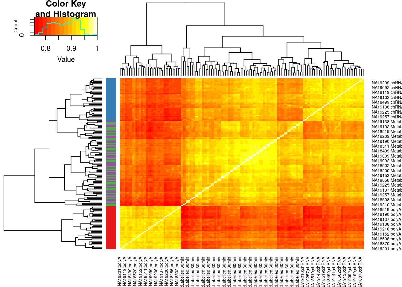

PlotColorKey(Colors$Key)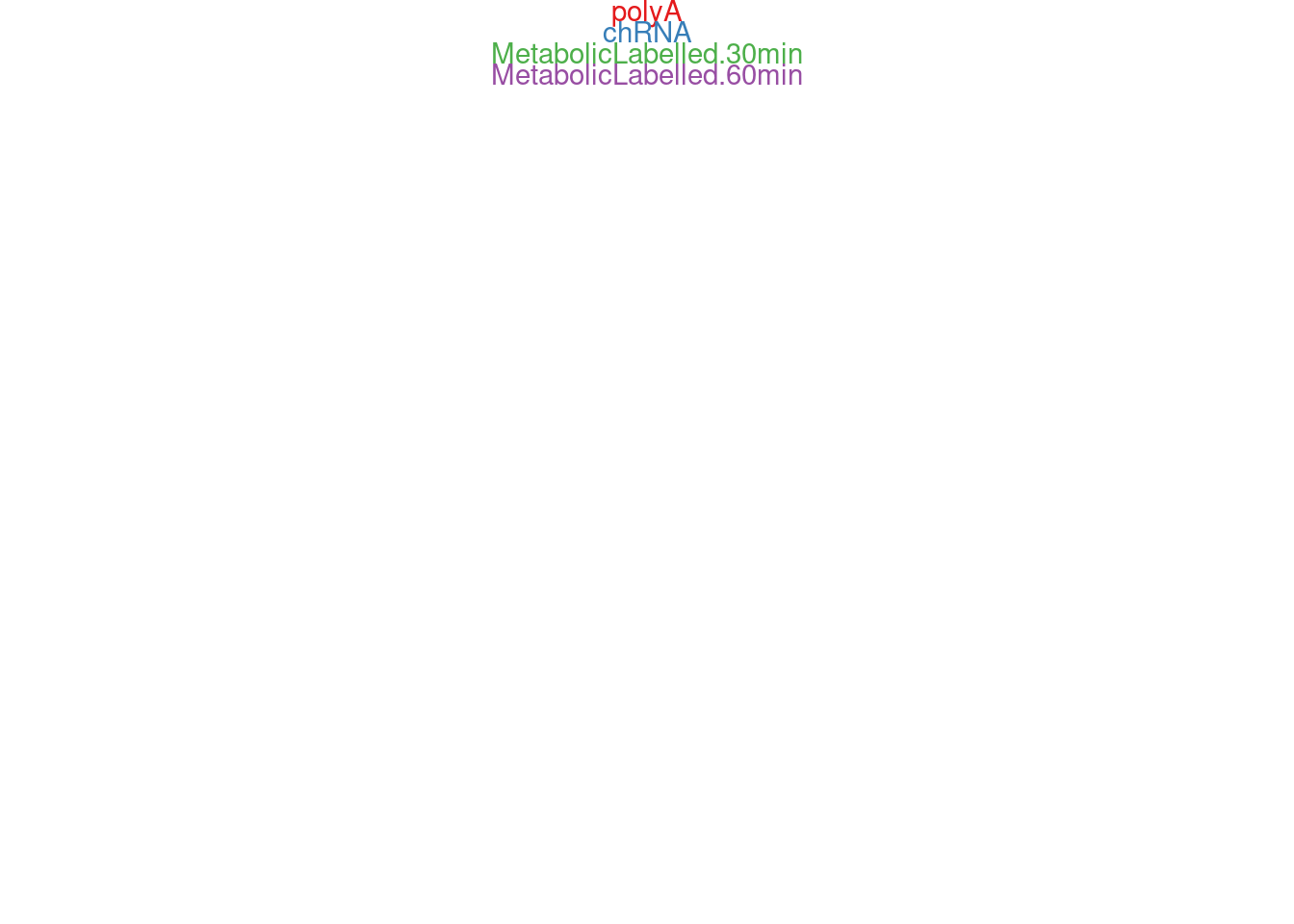

Plot intronic expression correlation heatmap

Colors <- ConvertToColorVector(colnames(dat.intronic.expression.rpkm) %>% str_replace(".+?;(.+?)", "\\1"))

cor(dat.intronic.expression.rpkm) %>%
  heatmap.2(trace='none', RowSideColors = Colors$ColorVector)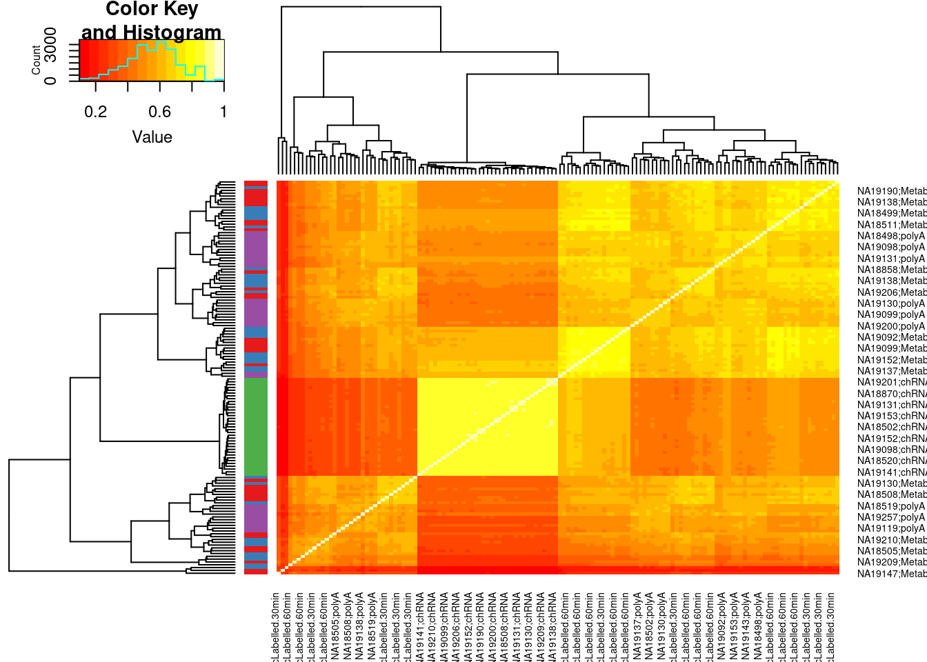

PlotColorKey(Colors$Key)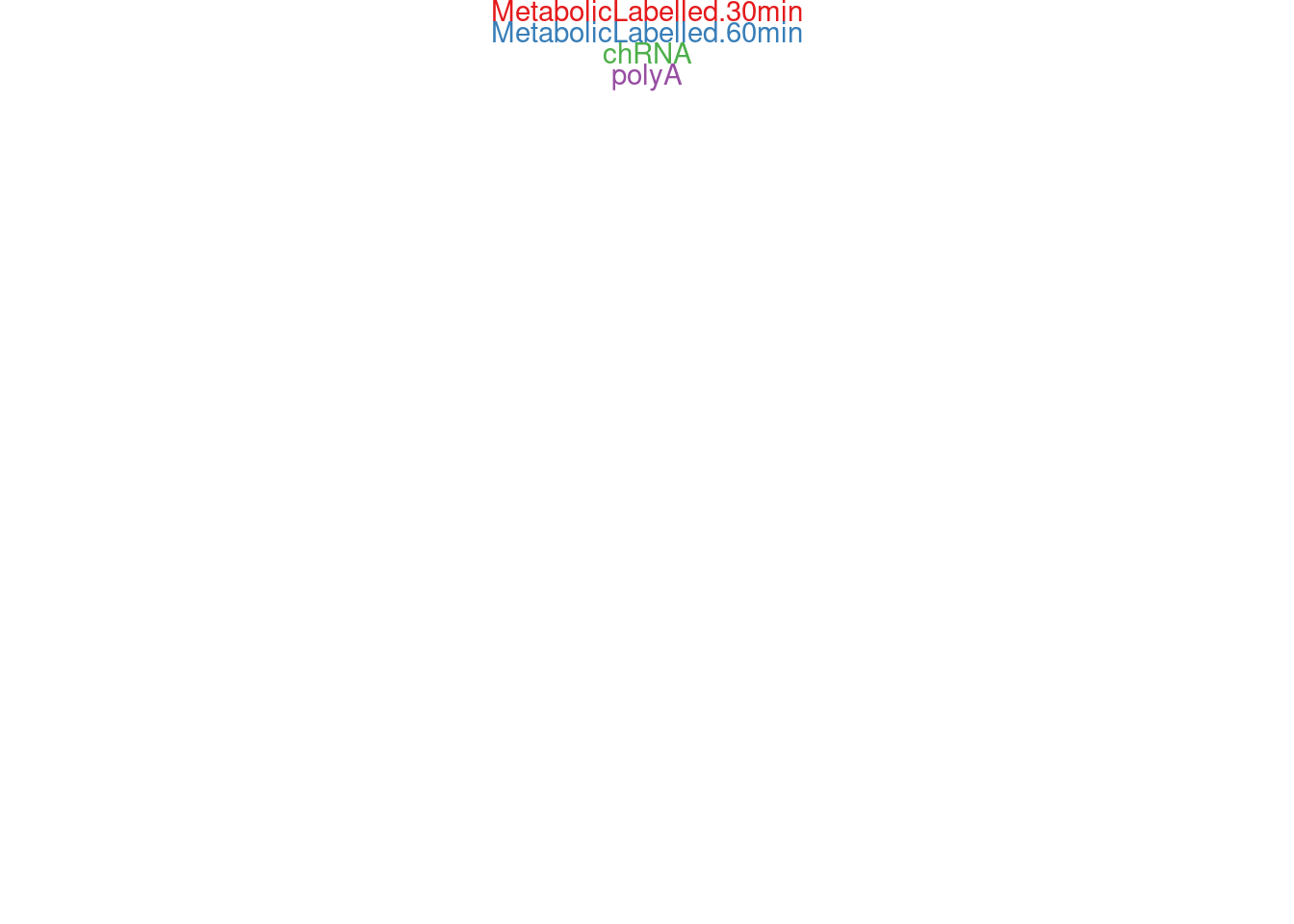

Plot them all together…

dat.combined.rpkm <- inner_join(
  dat.intronic.expression.rpkm %>%
    as.data.frame() %>%
    rownames_to_column("Geneid") %>%
    dplyr::rename_with(~paste0(.x, ";Intronic"), contains("NA")),
  dat.exonic.expression.rpkm %>%
    as.data.frame() %>%
    rownames_to_column("Geneid") %>%
    dplyr::rename_with(~paste0(.x, ";Exonic"), contains("NA")),
  by="Geneid"
)

ReorderedCols <- dat.combined.rpkm %>%
  dplyr::select(contains("NA")) %>%
  colnames() %>%
  as.data.frame() %>%
  separate(".", into=c("IndID", "Dataset", "Type"), sep=";") %>%
  mutate(Dataset = factor(Dataset, levels=c("chRNA","MetabolicLabelled.30min", "MetabolicLabelled.60min", "polyA"))) %>%
  arrange(Type, Dataset, IndID) %>%
  unite(Name, 1:3, sep=";") %>%
  pull(Name)

dat.combined.rpkm <- dat.combined.rpkm %>%
  dplyr::select(Geneid, all_of(ReorderedCols)) %>%
  column_to_rownames("Geneid")

Colors <- ConvertToColorVector(colnames(dat.combined.rpkm) %>% str_replace(".+?;(.+?);(.+?)", "\\1;\\2"))

cor(dat.combined.rpkm, method='p') %>%
  heatmap.2(trace='none', Rowv=F,Colv=F, RowSideColors = Colors$ColorVector, ColSideColors = Colors$ColorVector)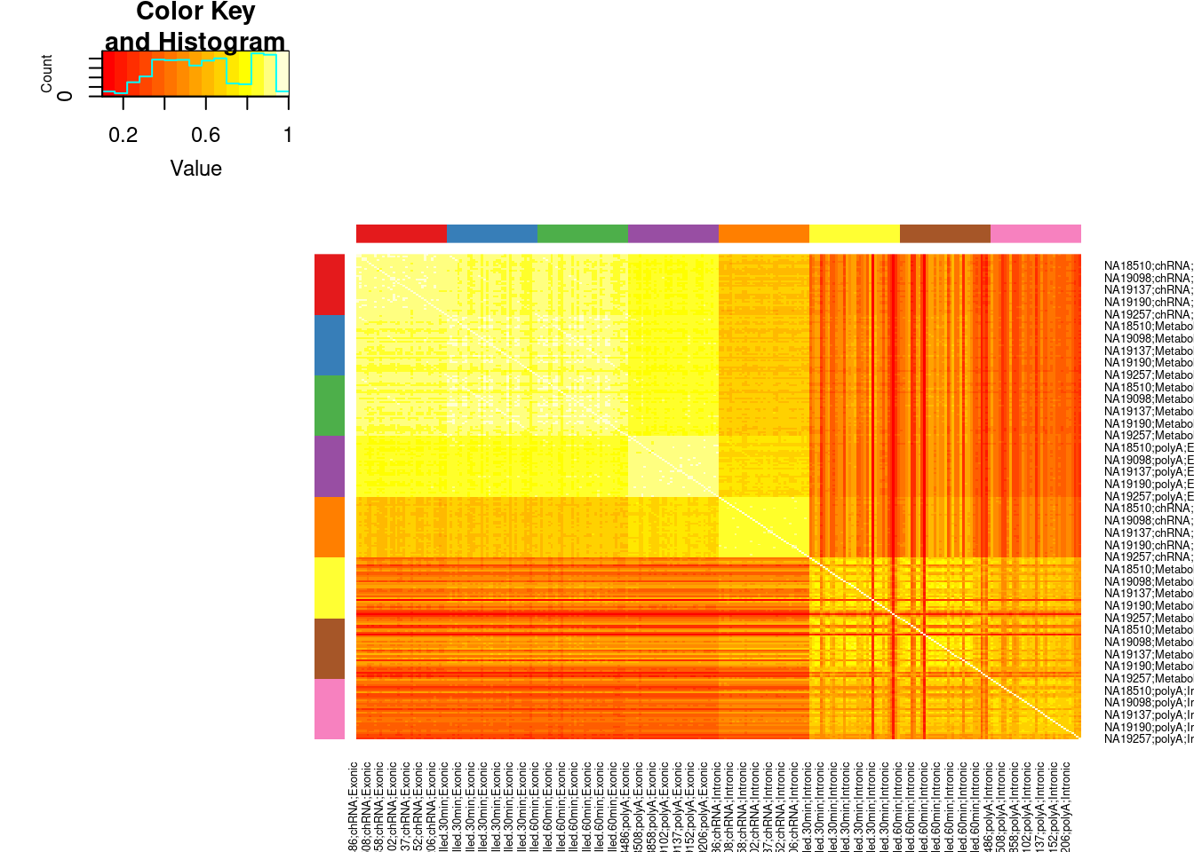

PlotColorKey(Colors$Key)

Ok, so the chRNA intronic in general correlates well with exonic measurements, while intronic measurements from the other ones do not correlate well. I’m a bit surprised at that the chRNA intronic is closer to polyA exonic than metabolic labelled exonic or chRNA exonic.

Does it make sense to look at these same correlation matrices after standardizing and normalizing the table? I think so. Let’s just try it…

scale_this <- function(x){
  (x - mean(x, na.rm=TRUE)) / sd(x, na.rm=TRUE)
}

dat.Normalized <- dat.combined.rpkm %>%
  rownames_to_column("Geneid") %>%
  gather("SampleName", "rpkm", -Geneid) %>%
  separate(SampleName, into=c("IndID", "dataset", "Type"), sep=";") %>%
  group_by(dataset, Type, Geneid) %>%
  mutate(scaled_rpkm = scale_this(rpkm)) %>%
  ungroup() %>%
  group_by(dataset, Type, IndID) %>%
  mutate(scaled_rpkm_percentiles = min_rank(scaled_rpkm)/(n()+1)) %>%
  mutate(ScaledAndInverseNormalized = qnorm(scaled_rpkm_percentiles)) %>%
  ungroup() %>%
  unite(SampleName, IndID, dataset, Type, sep=";") %>%
  dplyr::select(Geneid, SampleName, ScaledAndInverseNormalized) %>%
  pivot_wider(names_from="SampleName", values_from="ScaledAndInverseNormalized") %>%
  dplyr::select(Geneid, all_of(ReorderedCols)) %>%
  column_to_rownames("Geneid")



Colors <- ConvertToColorVector(colnames(dat.Normalized) %>% str_replace(".+?;(.+?);(.+?)", "\\1;\\2"))

cor(dat.Normalized, method='s') %>%
  heatmap.2(trace='none', Rowv=F,Colv=F, RowSideColors = Colors$ColorVector, ColSideColors = Colors$ColorVector)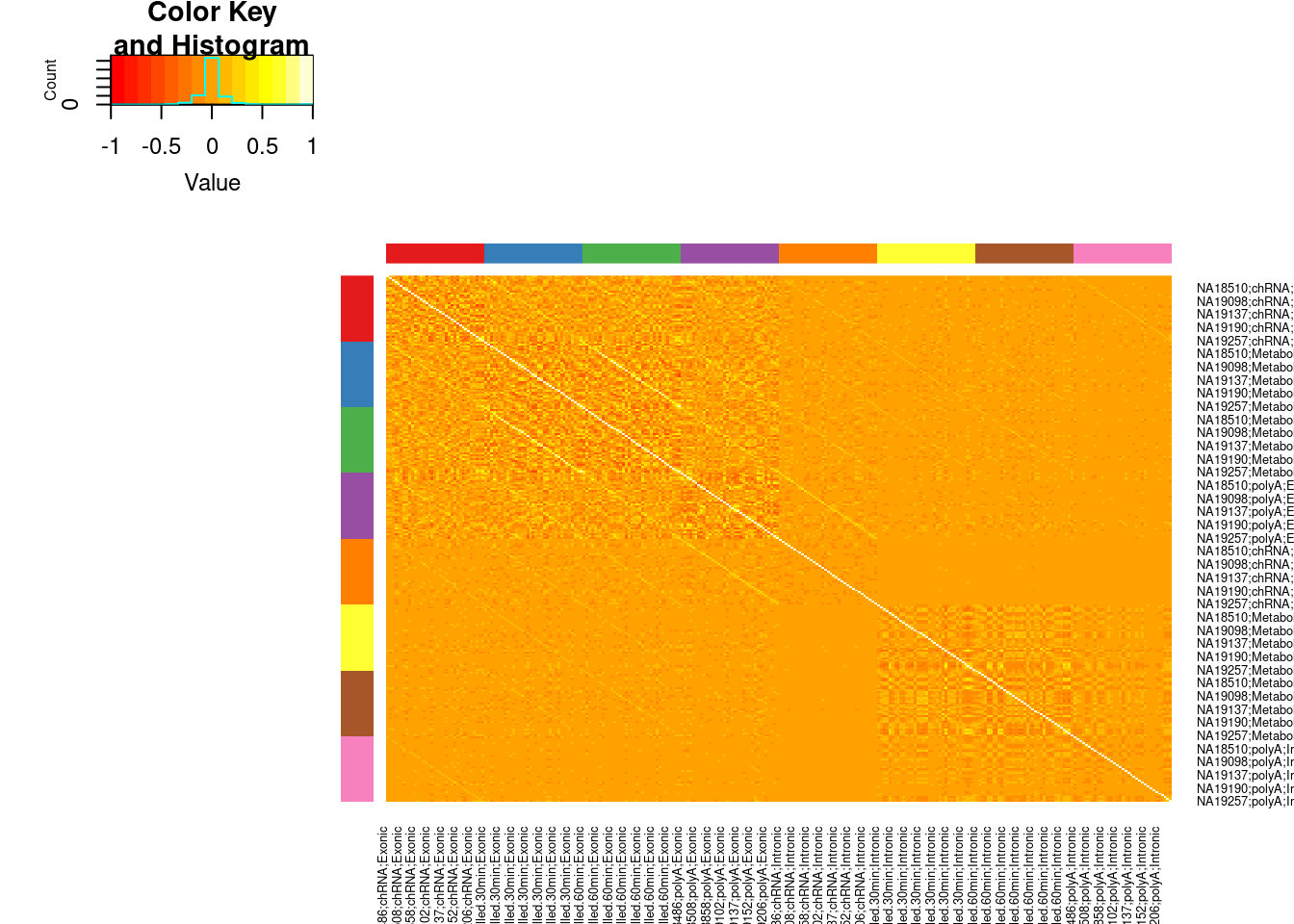

PlotColorKey(Colors$Key)

Ok, keep in mind I kept the order of individuals the same in each of the [assay];[Intron|Exon] boxes. So the diagonal streaks make sense. I think the genetic signals I would pick up in the chRNA intronic region will generally similar to ones in the exonic.

Let me plot what I’m trying to say in a more intuitive way:

BetweenVsWithinIndividualCorrelations <- cor(dat.Normalized, method='s') %>%
  as.data.frame() %>%
  rownames_to_column("SampleA") %>%
  gather("SampleB", "CorrelationCoef", contains("NA")) %>%
  separate(SampleA, into=c("IndID.A", "Assay.A"), sep=";", remove=F, extra="merge") %>%
  separate(SampleB, into=c("IndID.B", "Assay.B"), sep=";", remove=F, extra="merge") %>%
  mutate(Comparison = if_else(IndID.A == IndID.B, "WithinIndividual", "BetweenIndividual"))

ggplot(BetweenVsWithinIndividualCorrelations, aes(x=CorrelationCoef, color=Comparison)) +
  stat_ecdf() +
  facet_grid(rows=vars(Assay.A), cols=vars(Assay.B)) +
  theme_bw() +
  labs(y="ecdf", x="Distribution of spearman correlation coef") +
  theme(strip.text = element_text(size = 5))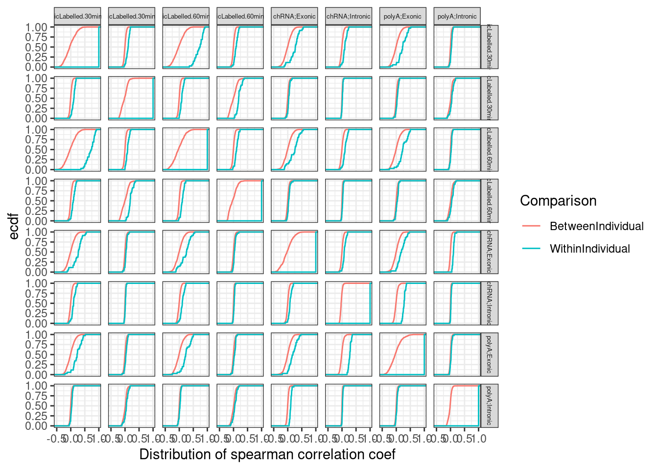

BetweenVsWithinIndividualCorrelations %>%
  group_by(Assay.A, Assay.B, Comparison) %>%
  summarise(medianCorr = median(CorrelationCoef)) %>%
  ungroup() %>%
  pivot_wider(names_from="Comparison", values_from="medianCorr") %>%
  mutate(DifferenceInMedian = WithinIndividual-BetweenIndividual) %>%
  ggplot(aes(x=Assay.A, y=Assay.B, fill=DifferenceInMedian)) +
  geom_raster() +
  scale_fill_viridis_c() +
  theme_classic()

`summarise()` has grouped output by 'Assay.A', 'Assay.B'. You can override
using the `.groups` argument.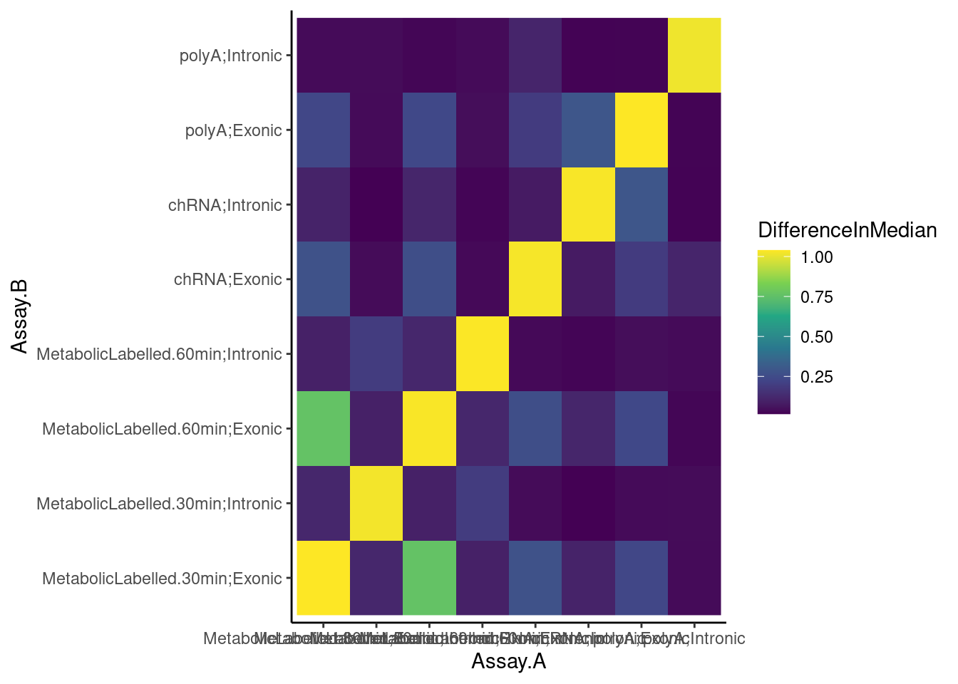

BetweenVsWithinIndividualCorrelations %>%
  group_by(Assay.A, Assay.B, Comparison) %>%
  summarise(medianCorr = median(CorrelationCoef)) %>%
  ungroup() %>%
  pivot_wider(names_from="Comparison", values_from="medianCorr") %>%
  mutate(DifferenceInMedian = WithinIndividual-BetweenIndividual) %>%
  dplyr::select(Assay.A, Assay.B, DifferenceInMedian) %>%
  pivot_wider(names_from="Assay.B", values_from="DifferenceInMedian") %>%
  column_to_rownames("Assay.A") %>%
  as.matrix() %>%
  heatmap.2(trace="none", col=viridis(50, direction = -1), cexRow=0.5, cexCol=0.5)

`summarise()` has grouped output by 'Assay.A', 'Assay.B'. You can override
using the `.groups` argument.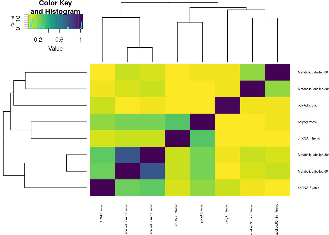

Ok, so the median difference between within-individual correlation vs between-individual correlation is greater between chRNA-intronic and polyA-exonic than chRNA-intronic and chRNA-exonic. All that is to say, I think the chRNA intronic gene expression, moreso than the chRNA exonic gene expression, is measuring something similar to polyA exonic gene expression. I think the chRNA intronic gene expression sum is might better read out for transcription than the chRNA exonic.

Session information

sessionInfo()

R version 3.6.1 (2019-07-05)
Platform: x86_64-pc-linux-gnu (64-bit)
Running under: CentOS Linux 7 (Core)

Matrix products: default
BLAS/LAPACK: /software/openblas-0.2.19-el7-x86_64/lib/libopenblas_haswellp-r0.2.19.so

locale:
 [1] LC_CTYPE=en_US.UTF-8 LC_NUMERIC=C         LC_TIME=C           
 [4] LC_COLLATE=C         LC_MONETARY=C        LC_MESSAGES=C       
 [7] LC_PAPER=C           LC_NAME=C            LC_ADDRESS=C        
[10] LC_TELEPHONE=C       LC_MEASUREMENT=C     LC_IDENTIFICATION=C 

attached base packages:
[1] stats     graphics  grDevices utils     datasets  methods   base     

other attached packages:
 [1] viridis_0.5.1      viridisLite_0.3.0  RColorBrewer_1.1-2 gplots_3.0.1.1    
 [5] edgeR_3.26.5       limma_3.40.6       forcats_0.4.0      stringr_1.4.0     
 [9] dplyr_1.0.9        purrr_0.3.4        readr_1.3.1        tidyr_1.2.0       
[13] tibble_3.1.7       ggplot2_3.3.6      tidyverse_1.3.0   

loaded via a namespace (and not attached):
 [1] Rcpp_1.0.5         locfit_1.5-9.1     lubridate_1.7.4    lattice_0.20-38   
 [5] gtools_3.9.2.2     assertthat_0.2.1   rprojroot_2.0.2    digest_0.6.20     
 [9] utf8_1.1.4         R6_2.4.0           cellranger_1.1.0   backports_1.4.1   
[13] reprex_0.3.0       evaluate_0.15      highr_0.9          httr_1.4.4        
[17] pillar_1.7.0       rlang_1.0.5        readxl_1.3.1       gdata_2.18.0      
[21] rstudioapi_0.14    rmarkdown_1.13     labeling_0.3       munsell_0.5.0     
[25] broom_1.0.0        compiler_3.6.1     httpuv_1.5.1       modelr_0.1.8      
[29] xfun_0.31          pkgconfig_2.0.2    htmltools_0.5.3    tidyselect_1.1.2  
[33] gridExtra_2.3      workflowr_1.6.2    fansi_0.4.0        crayon_1.3.4      
[37] dbplyr_1.4.2       withr_2.5.0        later_0.8.0        bitops_1.0-6      
[41] grid_3.6.1         jsonlite_1.6       gtable_0.3.0       lifecycle_1.0.1   
[45] DBI_1.1.0          git2r_0.26.1       magrittr_1.5       scales_1.1.0      
[49] KernSmooth_2.23-15 cli_3.3.0          stringi_1.4.3      farver_2.1.0      
[53] fs_1.5.2           promises_1.0.1     xml2_1.3.2         ellipsis_0.3.2    
[57] generics_0.1.3     vctrs_0.4.1        tools_3.6.1        glue_1.6.2        
[61] hms_0.5.3          fastmap_1.1.0      yaml_2.2.0         colorspace_1.4-1  
[65] caTools_1.17.1.2   rvest_0.3.5        knitr_1.39         haven_2.3.1