Does intron retention down regulate gene expression
Last updated: 2022-10-19
Checks: 6 1
Knit directory: ChromatinSplicingQTLs/analysis/
This reproducible R Markdown analysis was created with workflowr (version 1.6.2). The Checks tab describes the reproducibility checks that were applied when the results were created. The Past versions tab lists the development history.
The R Markdown file has unstaged changes. To know which version of the R Markdown file created these results, you’ll want to first commit it to the Git repo. If you’re still working on the analysis, you can ignore this warning. When you’re finished, you can run wflow_publish to commit the R Markdown file and build the HTML.
Great job! The global environment was empty. Objects defined in the global environment can affect the analysis in your R Markdown file in unknown ways. For reproduciblity it’s best to always run the code in an empty environment.
The command set.seed(20191126) was run prior to running the code in the R Markdown file. Setting a seed ensures that any results that rely on randomness, e.g. subsampling or permutations, are reproducible.
Great job! Recording the operating system, R version, and package versions is critical for reproducibility.
Nice! There were no cached chunks for this analysis, so you can be confident that you successfully produced the results during this run.
Great job! Using relative paths to the files within your workflowr project makes it easier to run your code on other machines.
Great! You are using Git for version control. Tracking code development and connecting the code version to the results is critical for reproducibility.
The results in this page were generated with repository version ef85e53. See the Past versions tab to see a history of the changes made to the R Markdown and HTML files.
Note that you need to be careful to ensure that all relevant files for the analysis have been committed to Git prior to generating the results (you can use wflow_publish or wflow_git_commit). workflowr only checks the R Markdown file, but you know if there are other scripts or data files that it depends on. Below is the status of the Git repository when the results were generated:
Ignored files:
    Ignored:    .DS_Store
    Ignored:    .Rhistory
    Ignored:    .Rproj.user/
    Ignored:    analysis/.Rhistory
    Ignored:    code/.DS_Store
    Ignored:    code/.RData
    Ignored:    code/._.DS_Store
    Ignored:    code/._README.md
    Ignored:    code/._report.html
    Ignored:    code/.ipynb_checkpoints/
    Ignored:    code/.snakemake/
    Ignored:    code/APA_Processing/
    Ignored:    code/Alignments/
    Ignored:    code/ChromHMM/
    Ignored:    code/ENCODE/
    Ignored:    code/ExpressionAnalysis/
    Ignored:    code/FastqFastp/
    Ignored:    code/FastqFastpSE/
    Ignored:    code/Genotypes/
    Ignored:    code/H3K36me3_CutAndTag.pdf
    Ignored:    code/IntronSlopes/
    Ignored:    code/Metaplots/
    Ignored:    code/Misc/
    Ignored:    code/MiscCountTables/
    Ignored:    code/Multiqc/
    Ignored:    code/Multiqc_chRNA/
    Ignored:    code/NonCodingRNA_annotation/
    Ignored:    code/PeakCalling/
    Ignored:    code/Phenotypes/
    Ignored:    code/PlotGruberQTLs/
    Ignored:    code/PlotQTLs/
    Ignored:    code/ProCapAnalysis/
    Ignored:    code/QC/
    Ignored:    code/QTL_SNP_Enrichment/
    Ignored:    code/QTLs/
    Ignored:    code/ReferenceGenome/
    Ignored:    code/Rplots.pdf
    Ignored:    code/Session.vim
    Ignored:    code/SplicingAnalysis/
    Ignored:    code/TODO
    Ignored:    code/Tehranchi/
    Ignored:    code/bigwigs/
    Ignored:    code/bigwigs_FromNonWASPFilteredReads/
    Ignored:    code/config/.DS_Store
    Ignored:    code/config/._.DS_Store
    Ignored:    code/config/.ipynb_checkpoints/
    Ignored:    code/debug.ipynb
    Ignored:    code/debug_python.ipynb
    Ignored:    code/deepTools/
    Ignored:    code/featureCounts/
    Ignored:    code/gwas_summary_stats/
    Ignored:    code/hyprcoloc/
    Ignored:    code/igv_session.xml
    Ignored:    code/log
    Ignored:    code/logs/
    Ignored:    code/notebooks/.ipynb_checkpoints/
    Ignored:    code/pi1/
    Ignored:    code/rules/.CreateUnstandardizedPhenotypeMatrices.smk.swp
    Ignored:    code/rules/.ipynb_checkpoints/
    Ignored:    code/rules/OldRules/
    Ignored:    code/rules/notebooks/
    Ignored:    code/scratch/
    Ignored:    code/scripts/.ipynb_checkpoints/
    Ignored:    code/scripts/GTFtools_0.8.0/
    Ignored:    code/scripts/__pycache__/
    Ignored:    code/scripts/liftOverBedpe/liftOverBedpe.py
    Ignored:    code/snakemake.log
    Ignored:    code/snakemake.sbatch.log
    Ignored:    code/test.introns.bed
    Ignored:    code/test.introns2.bed
    Ignored:    data/.DS_Store
    Ignored:    data/._.DS_Store
    Ignored:    data/._20220414203249_JASPAR2022_combined_matrices_25818_jaspar.txt
    Ignored:    data/GWAS_catalog_summary_stats_sources/._list_gwas_summary_statistics_6_Apr_2022-10.csv
    Ignored:    data/GWAS_catalog_summary_stats_sources/._list_gwas_summary_statistics_6_Apr_2022-11.csv
    Ignored:    data/GWAS_catalog_summary_stats_sources/._list_gwas_summary_statistics_6_Apr_2022-2.csv
    Ignored:    data/GWAS_catalog_summary_stats_sources/._list_gwas_summary_statistics_6_Apr_2022-3.csv
    Ignored:    data/GWAS_catalog_summary_stats_sources/._list_gwas_summary_statistics_6_Apr_2022-4.csv
    Ignored:    data/GWAS_catalog_summary_stats_sources/._list_gwas_summary_statistics_6_Apr_2022-5.csv
    Ignored:    data/GWAS_catalog_summary_stats_sources/._list_gwas_summary_statistics_6_Apr_2022-6.csv
    Ignored:    data/GWAS_catalog_summary_stats_sources/._list_gwas_summary_statistics_6_Apr_2022-7.csv
    Ignored:    data/GWAS_catalog_summary_stats_sources/._list_gwas_summary_statistics_6_Apr_2022-8.csv
    Ignored:    data/GWAS_catalog_summary_stats_sources/._list_gwas_summary_statistics_6_Apr_2022.csv

Untracked files:
    Untracked:  analysis/20221016_ExplorePSI_alternatives.Rmd
    Untracked:  analysis/20221019_PlotFigs1.Rmd
    Untracked:  code/rules/CreateUnstandardizedPhenotypeMatrices.smk
    Untracked:  code/scripts/PrepareLogCPM_PhenotypeTables.R
    Untracked:  code/scripts/PrepareLogRPKM_H3K36ME3_PhenotypeTables.R
    Untracked:  code/scripts/PrepareLogRPKM_PhenotypeTables.R
    Untracked:  code/scripts/PrepareUnstandardizedPSIPhenotypeTables.R
    Untracked:  code/scripts/Subset_YRI.R
    Untracked:  code/snakemake_profiles/slurm/__pycache__/

Unstaged changes:
    Modified:   analysis/20220928_ExploreIntronSum.Rmd
    Modified:   analysis/20221011_PlotHeatmapManyWays_ncRNA_Updated.Rmd
    Modified:   analysis/20221012_IntronRetentionAndExpressionConcordance.Rmd
    Modified:   code/Snakefile
    Modified:   code/envs/bedparse.yml
    Modified:   code/rules/ExpressionAnalysis.smk
    Modified:   code/rules/Metaplots.smk
    Modified:   code/rules/QTLTools.smk
    Modified:   code/rules/SplicingAnalysis.smk
    Modified:   code/scripts/CalculatePi1_GetAscertainmentP_AllPairs.py
    Modified:   code/scripts/CalculatePi1_GetTraitPairs_AllTraits.R
    Modified:   code/scripts/GenometracksByGenotype
    Modified:   code/scripts/MakeBigwigList.R
    Modified:   code/scripts/MakeNormalizedPSI.Tables.R
Note that any generated files, e.g. HTML, png, CSS, etc., are not included in this status report because it is ok for generated content to have uncommitted changes.
These are the previous versions of the repository in which changes were made to the R Markdown (analysis/20221012_IntronRetentionAndExpressionConcordance.Rmd) and HTML (docs/20221012_IntronRetentionAndExpressionConcordance.html) files. If you’ve configured a remote Git repository (see ?wflow_git_remote), click on the hyperlinks in the table below to view the files as they were in that past version.
| File | Version | Author | Date | Message |
|---|---|---|---|---|
| Rmd | ef85e53 | Benjmain Fair | 2022-10-12 | update index |
| Rmd | 3201a19 | Benjmain Fair | 2022-10-12 | add IR notebook |
| html | 3201a19 | Benjmain Fair | 2022-10-12 | add IR notebook |
Intro
I previously showed that effect size directions for intron retention QTLs puzzingly positively correct with eQTLs (more intron retention = more expression). Somehow I think intron retention QTLs are often picking up on chromatin effects. Let’s break up the intron retention QTLs into groups by the location of the SNP (in a enhancer/promoter vs a splice site) and reassess the concordance of expression effects. I can also look at the same idea with normal leafcutter sQTLs, comparing introns by their annotation type. For example increase in splicing of annotated or “basic” tagged introns might generally increase expression, versus increase in unannoated or “NMD” tagged introns might decrease expression.
library(tidyverse)
library(data.table)
library(qvalue)
First let’s make some basic plots establishing that chRNA has more unannoated and NMD-specific splicing.
NMD.transcript.introns <- read_tsv("../code/SplicingAnalysis/Annotations/NMD/NMD_trancsript_introns.bed.gz", col_names=c("chrom", "start", "stop", "name", "score", "strand")) %>%
  mutate(stop=stop+1) %>%
  unite(intron, chrom:stop, strand)

Non.NMD.transcript.introns <- read_tsv("../code/SplicingAnalysis/Annotations/NMD/NonNMD_trancsript_introns.bed.gz", col_names=c("chrom", "start", "stop", "name", "score", "strand")) %>%
  mutate(stop=stop+1) %>%
  unite(intron, chrom:stop, strand)


NMD.specific.introns <- setdiff(NMD.transcript.introns$intron, Non.NMD.transcript.introns$intron)


SpliceJunctionCountTables <- Sys.glob("../code/SplicingAnalysis/leafcutter/NormalizedPsiTables/PSI.JunctionCounts.*.bed.gz") %>%
  setNames(str_replace(., "../code/SplicingAnalysis/leafcutter/NormalizedPsiTables/PSI.JunctionCounts.(.+?).bed.gz", "\\1")) %>%
  lapply(read_tsv)

lapply(SpliceJunctionCountTables, dim)
$Expression.Splicing
[1] 198246 468
$MetabolicLabelled.30min
[1] 198246 72
$MetabolicLabelled.60min
[1] 198246 72
$chRNA.Expression.Splicing
[1] 198246 93SpliceJunctionCountTables$Expression.Splicing %>%
mutate(Intron=paste(`#Chrom`, start, end, strand, sep="_")) %>%
mutate(Is.NMD.Intron = Intron %in% NMD.specific.introns) %>%
group_by(Is.NMD.Intron) %>%
summarise_if(is.numeric, sum, na.rm = TRUE) %>%
dplyr::select(-start, -end) %>%
column_to_rownames("Is.NMD.Intron") %>%
t() FALSE TRUE
HG00096 3709149 17830
HG00097 5970288 25340
HG00099 3264484 12455
HG00100 3341315 12673
HG00101 3014382 13597
HG00102 2798030 12136
HG00103 3493738 16343
HG00104 3198591 17035
HG00105 6660181 26858
HG00106 4213349 16764
HG00108 5343418 25128
HG00109 2476507 9483
HG00110 5874235 25022
HG00111 5103426 19924
HG00112 3954505 17357
HG00114 3143081 13341
HG00115 4159089 18277
HG00116 4459861 16656
HG00117 7020550 34687
HG00118 4452455 21158
HG00119 4819485 22125
HG00120 1971592 9648
HG00121 2799478 12366
HG00122 4555019 18539
HG00123 5037802 19918
HG00124 4624537 19468
HG00125 2934475 13474
HG00126 4763900 20625
HG00127 5040019 20127
HG00128 3499064 13486
HG00129 3831033 16600
HG00130 4438788 16820
HG00131 4378333 22526
HG00132 5803042 21307
HG00133 4032972 18635
HG00134 6118321 27548
HG00135 2042680 8802
HG00136 4249736 18012
HG00137 3478431 17251
HG00138 4193157 16761
HG00139 5748104 24970
HG00141 5762495 23982
HG00142 3812175 18077
HG00143 3806730 14021
HG00145 4494523 18326
HG00146 4306866 24053
HG00148 3018315 12151
HG00149 3902925 18418
HG00150 4436945 19361
HG00151 2447286 8044
HG00152 7448106 38066
HG00154 4705735 22636
HG00155 2685738 11240
HG00156 3679685 14311
HG00157 5741376 24613
HG00158 4009332 18344
HG00159 5021558 17151
HG00160 2505076 10112
HG00171 2032306 7776
HG00173 2191587 8847
HG00174 3941240 16968
HG00176 3667589 14634
HG00177 4116980 18940
HG00178 4534062 20179
HG00179 3205059 12474
HG00180 4628325 20671
HG00181 3650049 16708
HG00182 3382004 17015
HG00183 4358898 21750
HG00185 4446719 17583
HG00186 2270761 8636
HG00187 5107996 22778
HG00188 4646271 21645
HG00189 3308923 14809
HG00231 4370995 14095
HG00232 2313245 13634
HG00233 4750956 25677
HG00234 6830836 33353
HG00235 2924441 13550
HG00236 5054446 23572
HG00238 4413807 19029
HG00239 5314160 25755
HG00240 5893909 23249
HG00242 3467779 14811
HG00243 4132949 17434
HG00244 4897465 21724
HG00245 4142296 20418
HG00246 4937568 19255
HG00247 4079683 16616
HG00249 2465695 8834
HG00250 3021206 13199
HG00251 4917143 18681
HG00252 3713856 13296
HG00253 4936315 17540
HG00255 4617945 20945
HG00256 5099634 18872
HG00257 3665301 17242
HG00258 3895815 14408
HG00259 7911053 37589
HG00260 4667808 26120
HG00261 4537491 19724
HG00262 5856944 24388
HG00263 4390463 18371
HG00264 3344525 13163
HG00265 4353067 17439
HG00266 5010139 23162
HG00267 4296377 18259
HG00268 4307832 19355
HG00269 3926061 16034
HG00271 6400367 21977
HG00272 4319763 18987
HG00273 2510226 8462
HG00274 4628827 18244
HG00275 3834973 17482
HG00276 6058418 24514
HG00277 3195087 14855
HG00278 3227170 15964
HG00280 3443262 17597
HG00281 4320498 17993
HG00282 4784231 17814
HG00284 4376866 17114
HG00285 3673413 18046
HG00306 3050528 17782
HG00308 2463042 9289
HG00309 8010977 37454
HG00310 4898982 18995
HG00311 3909493 17731
HG00312 7405868 30994
HG00313 4012941 15541
HG00315 5428181 22548
HG00319 3887748 18426
HG00320 4161739 16666
HG00321 4917234 22371
HG00323 2961773 12363
HG00324 4372388 18374
HG00325 4976154 24845
HG00326 4646613 17412
HG00327 2843277 11606
HG00328 5674146 20867
HG00329 1775654 7067
HG00330 4132218 15337
HG00331 4901185 26314
HG00332 4016403 24887
HG00334 4028498 18298
HG00335 4711437 19610
HG00336 3772473 15268
HG00337 3575607 15512
HG00338 7310290 27602
HG00339 4025943 17363
HG00341 4535953 17363
HG00342 4925542 20968
HG00343 5094171 23952
HG00344 3822899 21535
HG00345 3439202 13667
HG00346 5599558 19967
HG00349 3908654 16915
HG00350 2135650 8408
HG00351 2888931 10522
HG00353 3529837 15394
HG00355 6269425 27740
HG00356 5925857 21602
HG00358 3462158 16527
HG00359 3948910 16191
HG00360 3301681 13905
HG00361 4787098 23595
HG00362 3734270 17125
HG00364 5230488 19609
HG00365 8141836 39026
HG00366 4785057 22726
HG00367 5222882 19541
HG00369 4835865 21794
HG00371 3625286 14187
HG00372 4105444 18350
HG00373 5937275 27804
HG00375 4670034 21369
HG00376 4620808 19631
HG00377 5093916 18791
HG00378 5201981 22356
HG00379 52857 200
HG00380 2935953 11289
HG00381 1719664 7117
HG00382 4059788 17628
HG00383 4481158 18802
HG00384 6386093 30301
HG01334 6089787 21667
HG01789 3812203 17195
HG01790 1929228 6488
HG01791 4912019 18892
HG02215 4357410 16058
NA06984 2708135 11676
NA06985 4436740 16220
NA06986 4947141 19865
NA06989 3083551 12025
NA06994 5712127 24546
NA07037 3991273 17642
NA07048 3664840 16638
NA07051 3652844 15410
NA07056 3731176 16451
NA07346 4982321 16266
NA07347 4626890 20315
NA07357 3926419 17919
NA10847 4656732 17627
NA10851 3711762 13600
NA11829 3015970 10951
NA11830 3602959 14119
NA11831 5853937 24663
NA11832 5357051 19423
NA11840 4122582 14721
NA11843 4290776 18859
NA11881 4566621 16360
NA11892 3064872 15400
NA11893 5968405 30384
NA11894 5188518 19978
NA11918 3332691 12608
NA11920 4965471 19041
NA11930 2906896 13776
NA11931 3297081 11411
NA11992 3667446 13436
NA11993 5006117 17528
NA11994 6621933 22006
NA11995 3757594 15068
NA12004 2689434 10437
NA12005 4273209 17992
NA12006 4712133 17421
NA12043 4568353 13867
NA12044 4756870 19920
NA12045 2805376 10438
NA12058 4525160 20435
NA12144 5082748 19258
NA12154 3819808 12964
NA12155 3476005 11791
NA12156 4425007 20955
NA12234 4887260 20323
NA12249 3760956 11892
NA12272 2615984 10034
NA12273 4033963 18188
NA12275 4245904 20067
NA12282 2266286 8710
NA12283 3933023 15318
NA12286 4571418 19997
NA12287 2542428 10037
NA12340 4439386 19697
NA12341 4201906 16161
NA12342 3780276 15435
NA12347 4137411 17212
NA12348 2138806 7364
NA12383 3653658 15763
NA12399 1655077 6208
NA12400 3925633 12910
NA12413 5681034 19661
NA12489 4272378 17029
NA12546 2789900 9949
NA12716 11515675 48076
NA12717 3733058 14061
NA12718 4670146 20307
NA12749 3058040 13270
NA12750 4280818 16678
NA12751 5702382 21297
NA12760 2267191 7497
NA12761 4541986 18917
NA12762 3651656 13246
NA12763 4804979 19865
NA12775 6685775 32504
NA12776 4648704 21329
NA12777 3848971 16697
NA12778 3727973 14819
NA12812 2777345 11330
NA12813 4106195 16696
NA12814 6563804 28440
NA12815 4825636 18697
NA12827 2346154 9569
NA12829 5670688 23333
NA12830 2762144 9209
NA12842 5002673 20768
NA12843 3402590 13247
NA12872 5094271 18992
NA12873 4486308 17137
NA12874 3968589 17188
NA12889 5089067 20378
NA12890 3448926 15343
NA18486 6392603 29693
NA18487 3509994 15725
NA18488 2664882 11001
NA18489 4285770 16941
NA18498 5703609 22499
NA18499 4389402 19086
NA18502 8527863 34758
NA18505 2337208 8365
NA18508 3568030 12657
NA18510 3099265 13139
NA18511 7355949 36864
NA18517 2036033 6928
NA18519 3348557 11801
NA18520 3914753 12883
NA18858 4419347 16005
NA18861 2150847 8389
NA18867 3805544 15181
NA18868 4459176 16287
NA18870 3475632 13925
NA18873 4021058 18075
NA18907 2926979 11021
NA18908 5132520 20888
NA18909 4777260 19066
NA18910 2718491 8935
NA18912 6539369 24850
NA18916 6459892 26793
NA18917 3741327 16588
NA18923 4953481 18205
NA18933 3367847 12818
NA18934 7077478 30049
NA19092 4536589 18204
NA19093 5145790 18394
NA19095 6422144 22765
NA19096 3888047 15239
NA19098 6330312 27602
NA19099 5976613 20245
NA19102 3244244 12671
NA19107 4263857 17886
NA19108 7541158 32076
NA19113 2286263 8052
NA19114 4962358 17240
NA19116 6009816 24465
NA19117 4885102 20525
NA19118 6545544 24407
NA19119 2620952 10111
NA19121 3569276 14914
NA19129 3701726 16594
NA19130 4050529 16537
NA19131 5876765 25474
NA19137 3612162 14903
NA19138 2964898 12086
NA19141 4120838 18342
NA19143 5179458 18286
NA19144 2620186 9596
NA19146 5084546 22434
NA19147 6793799 28862
NA19149 3591796 16002
NA19150 4513741 18959
NA19152 4455900 19009
NA19153 3985531 15904
NA19159 12085171 55435
NA19160 2882162 9919
NA19171 4888230 20935
NA19172 4113566 14793
NA19175 4573481 20389
NA19184 5513791 22694
NA19185 4301998 16756
NA19189 5259112 21188
NA19190 4527256 19726
NA19197 2655390 12332
NA19198 5124685 20410
NA19200 4284716 14102
NA19201 4065061 18006
NA19204 3279983 13666
NA19206 5500752 21098
NA19207 4567051 20001
NA19209 3537760 15313
NA19210 3671149 13832
NA19213 5474128 20626
NA19214 4795815 18566
NA19222 5014274 19037
NA19223 6461058 28695
NA19225 3505683 13048
NA19235 4912111 22322
NA19236 3242259 14193
NA19247 4332756 18392
NA19248 4625652 16562
NA19256 4496254 19039
NA19257 5355988 18457
NA20502 3609428 13463
NA20503 3540626 13731
NA20504 3605850 16487
NA20505 5158963 19391
NA20506 3129044 14439
NA20507 3541199 18181
NA20508 4524233 15803
NA20509 8349744 34255
NA20510 2225638 8418
NA20512 3645431 13203
NA20513 4090869 17775
NA20514 3193367 16394
NA20515 5154752 25517
NA20516 4503303 17217
NA20517 3039969 13430
NA20518 4655493 18220
NA20519 4821993 22205
NA20520 2184890 6749
NA20521 3162387 13549
NA20524 4943563 18496
NA20525 3644787 14916
NA20527 5977643 26619
NA20528 4805622 21690
NA20529 4684125 17918
NA20530 5425699 29442
NA20531 4170078 19614
NA20532 2675278 11824
NA20534 5268093 21901
NA20535 3816371 14859
NA20536 3201797 12773
NA20537 2977027 11177
NA20538 2192032 9527
NA20539 3888629 17010
NA20540 2765585 12055
NA20541 4788497 19581
NA20542 2586825 11225
NA20543 4050804 13271
NA20544 4176707 15346
NA20581 3293928 12192
NA20582 5091495 22005
NA20585 2732358 11307
NA20586 4818464 16463
NA20588 4239713 23156
NA20589 2739576 9850
NA20752 5400758 20717
NA20754 3935155 14795
NA20756 4266291 16442
NA20757 4057917 16915
NA20758 6184580 24057
NA20759 3347631 16488
NA20760 2667378 12282
NA20761 3667974 16458
NA20765 6186872 28668
NA20766 3687854 14904
NA20768 4001112 17214
NA20769 3336409 13279
NA20770 2533934 9995
NA20771 4545077 16515
NA20772 4997333 28151
NA20773 3946830 15855
NA20774 2600558 11448
NA20778 1257095 5160
NA20783 5009501 18817
NA20785 3958258 15069
NA20786 5237921 15719
NA20787 4854000 25222
NA20790 4104832 14035
NA20792 4144541 15760
NA20795 5381487 22938
NA20796 6965737 28422
NA20797 6344504 26211
NA20798 3285299 13126
NA20799 4276502 19998
NA20800 5097081 21696
NA20801 5222605 19297
NA20802 3755236 13648
NA20803 7751162 26444
NA20804 4176025 16293
NA20805 2753391 12522
NA20806 2391712 12558
NA20807 4885933 20361
NA20808 4304608 17827
NA20809 4006770 16573
NA20810 5330072 20639
NA20811 3204473 14761
NA20812 4884054 16939
NA20813 5015426 22240
NA20814 4873701 18876
NA20815 5015517 18986
NA20816 4097123 18260
NA20819 2902477 13864
NA20826 3834408 14608
NA20828 6421596 32532Sum.NMD.Intron.Counts <- function(df){
df %>%
mutate(Intron=paste(`#Chrom`, start, end, strand, sep="_")) %>%
mutate(Is.NMD.Intron = Intron %in% NMD.specific.introns) %>%
group_by(Is.NMD.Intron) %>%
summarise_if(is.numeric, sum, na.rm = TRUE) %>%
dplyr::select(-start, -end) %>%
column_to_rownames("Is.NMD.Intron") %>%
t() %>%
as.data.frame() %>%
rownames_to_column("IndID") %>%
return()
}
lapply(SpliceJunctionCountTables, Sum.NMD.Intron.Counts) %>%
bind_rows(.id="Source") %>%
dplyr::rename(c("NotNMD"="FALSE", "NMD"="TRUE")) %>%
mutate(Fraction = NMD/(NMD+NotNMD)*100) %>%
ggplot(aes(x=Source, y=Fraction, color=Source)) +
geom_boxplot(outlier.position="none") +
geom_jitter() +
theme_bw()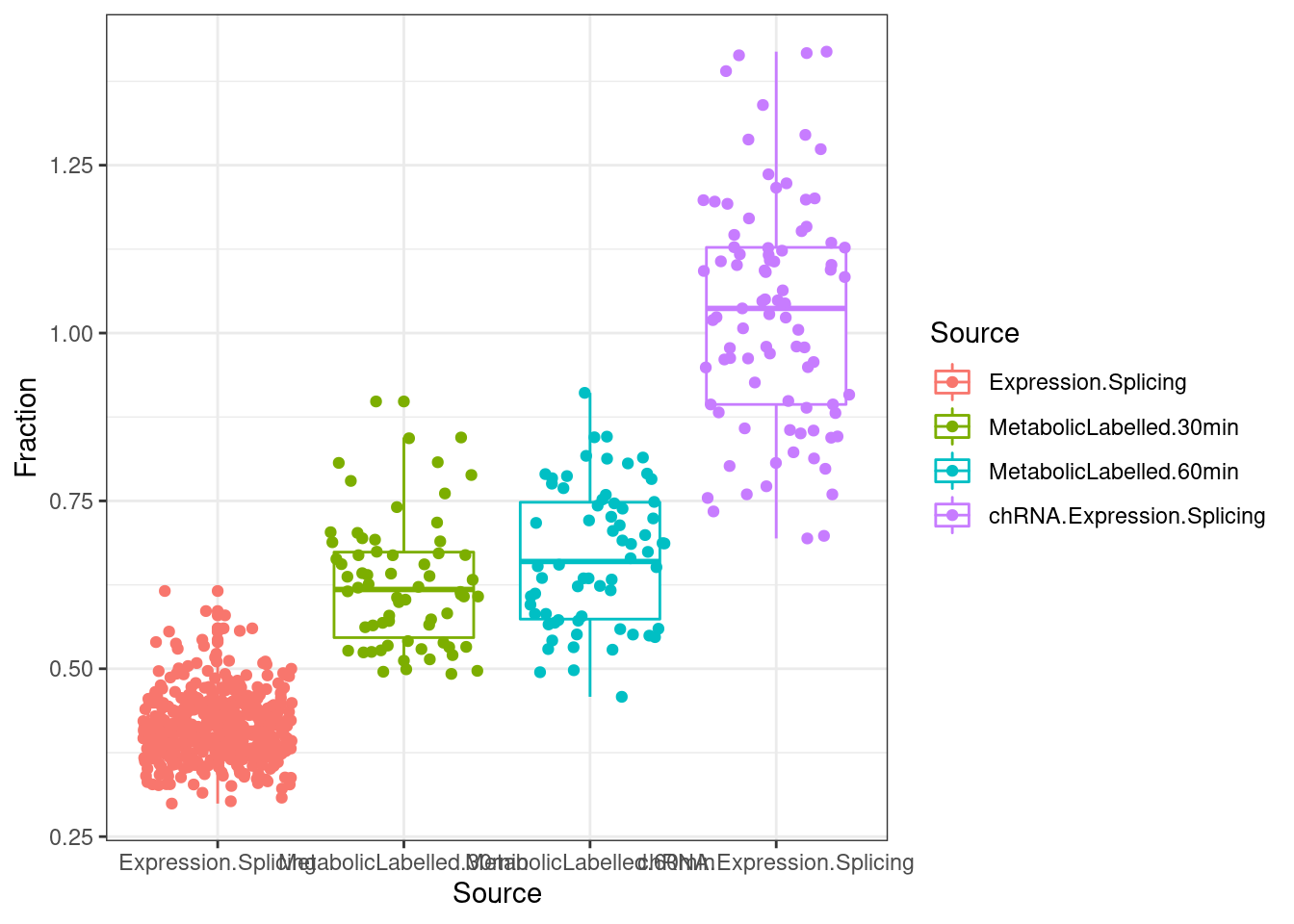
lapply(SpliceJunctionCountTables, Sum.NMD.Intron.Counts) %>%
  bind_rows(.id="Source") %>%
  dplyr::rename(c("NotNMD"="FALSE", "NMD"="TRUE")) %>%
  mutate(TotalJunctionCounts = NMD+NotNMD) %>%
  ggplot(aes(x=Source, y=TotalJunctionCounts, color=Source)) +
  geom_boxplot(outlier.position="none") +
  geom_jitter() +
  theme_bw() +
  labs(title="Total juncs per dataset", y="Total num juncs")
Hmmm, consistent with previous analysis with a smaller number of samples that I uniformly processed (trimmed reads to single end, constant read length across positions) has metabolic labelled was in between chRNA and polyA.
let’s prcoeed to reading in other files
PhenotypeAliases <- read_tsv("../data/Phenotypes_recode_for_Plotting.txt")

PC.ShortAliases <- PhenotypeAliases %>%
  dplyr::select(PC, ShorterAlias) %>% deframe()

coloc.results <- read_tsv("../code/hyprcoloc/Results/ForColoc/MolColocStandard/results.txt.gz")

coloc.results.tidycolocalized <- read_tsv("../code/hyprcoloc/Results/ForColoc/MolColocStandard/tidy_results_OnlyColocalized.txt.gz") %>%
  separate(phenotype_full, into=c("PC", "P"), sep=";")

finemap.snps.annotated <- read_tsv("../code/QTL_SNP_Enrichment/FinemapIntersections/MolColocStandard.bed.gz", col_names=c("SNPchrom", "SNPstart", "SNPstop", "SNP_iteration_locus", "FinemapPP", "AnnotationChrom", "AnnotationStart", "AnnotatioStop", "AnnotationClass", "Overlap")) %>%
  dplyr::select(-Overlap)
Count chromatin-colocalizing and splicing-colocalizing eQTLs, and recreate previous observation about concordant effects
coloc.results.tidycolocalized %>%
  group_by(Locus, snp) %>%
  filter(any(PC=="Expression.Splicing.Subset_YRI")) %>%
  summarise(
    ContainsChromatinEqtl = any(PC %in% c("H3K27AC", "H3K4ME1", "H3K4ME3")),
    ContainsSqtl = any(PC %in% c("polyA.Splicing.Subset_YRI", "chRNA.Splicing", "chRNA.IER"))
    ) %>%
  ggplot(aes(x=1, fill=paste(ContainsChromatinEqtl, ContainsSqtl))) +
  geom_bar() +
  labs(title="More chromatin localization with eQTLs than splicing", y="Number of colocalizing eQTLs") +
  theme_classic() +
  theme(axis.title.x=element_blank(),
        axis.text.x=element_blank(),
        axis.ticks.x=element_blank())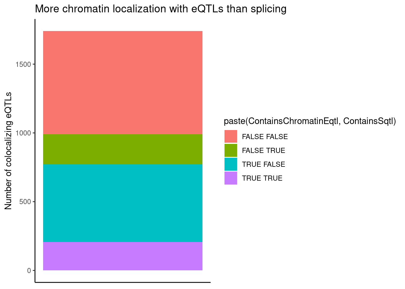
| Version | Author | Date |
|---|---|---|
| 3201a19 | Benjmain Fair | 2022-10-12 |
coloc.results.tidycolocalized %>%
  group_by(Locus, snp) %>%
  filter(any(PC=="Expression.Splicing.Subset_YRI")) %>%
  ungroup() %>%
  filter(PC %in% c("Expression.Splicing.Subset_YRI","H3K27AC", "H3K4ME1", "H3K4ME3", "polyA.Splicing.Subset_YRI", "chRNA.Splicing", "chRNA.IER")) %>%
  left_join(., ., by=c("Locus", "snp")) %>%
  filter(!((P.x == P.y) & (PC.x == PC.y))) %>%
  group_by(Locus, snp) %>%
  mutate(
    ContainsChromatinEqtl = any(PC.x %in% c("H3K27AC", "H3K4ME1", "H3K4ME3")),
    ContainsSqtl = any(PC.x %in% c("polyA.Splicing.Subset_YRI", "chRNA.Splicing", "chRNA.IER"))
    ) %>%
  ungroup() %>%
  mutate(Contains.eQTL_Contains.sQTL = paste(ContainsChromatinEqtl, ContainsSqtl)) %>%
  group_by(Contains.eQTL_Contains.sQTL, PC.x, PC.y) %>%
  summarise(cor = cor(beta.x, beta.y, method="spearman")) %>%
  mutate(PC.x = recode(PC.x, !!!PC.ShortAliases)) %>%
  mutate(PC.y = recode(PC.y, !!!PC.ShortAliases)) %>%
  ggplot(aes(x=PC.x, y=PC.y, fill=cor)) +
  geom_raster() +
  scale_fill_gradient2() +
  facet_wrap(~Contains.eQTL_Contains.sQTL) +
  scale_x_discrete(expand=c(0,0)) +
  scale_y_discrete(expand=c(0,0)) +
  theme_classic() +
  theme(axis.text.x = element_text(angle = 45, vjust = 1, hjust=1)) +
  labs(x="TraitA Phenotype class", y="TraitB Phenotype class", fill="Spearman cor", title="Effect size correlation",
       caption = "FacetTitle: IsChromatinQTL IsSplicingQTL")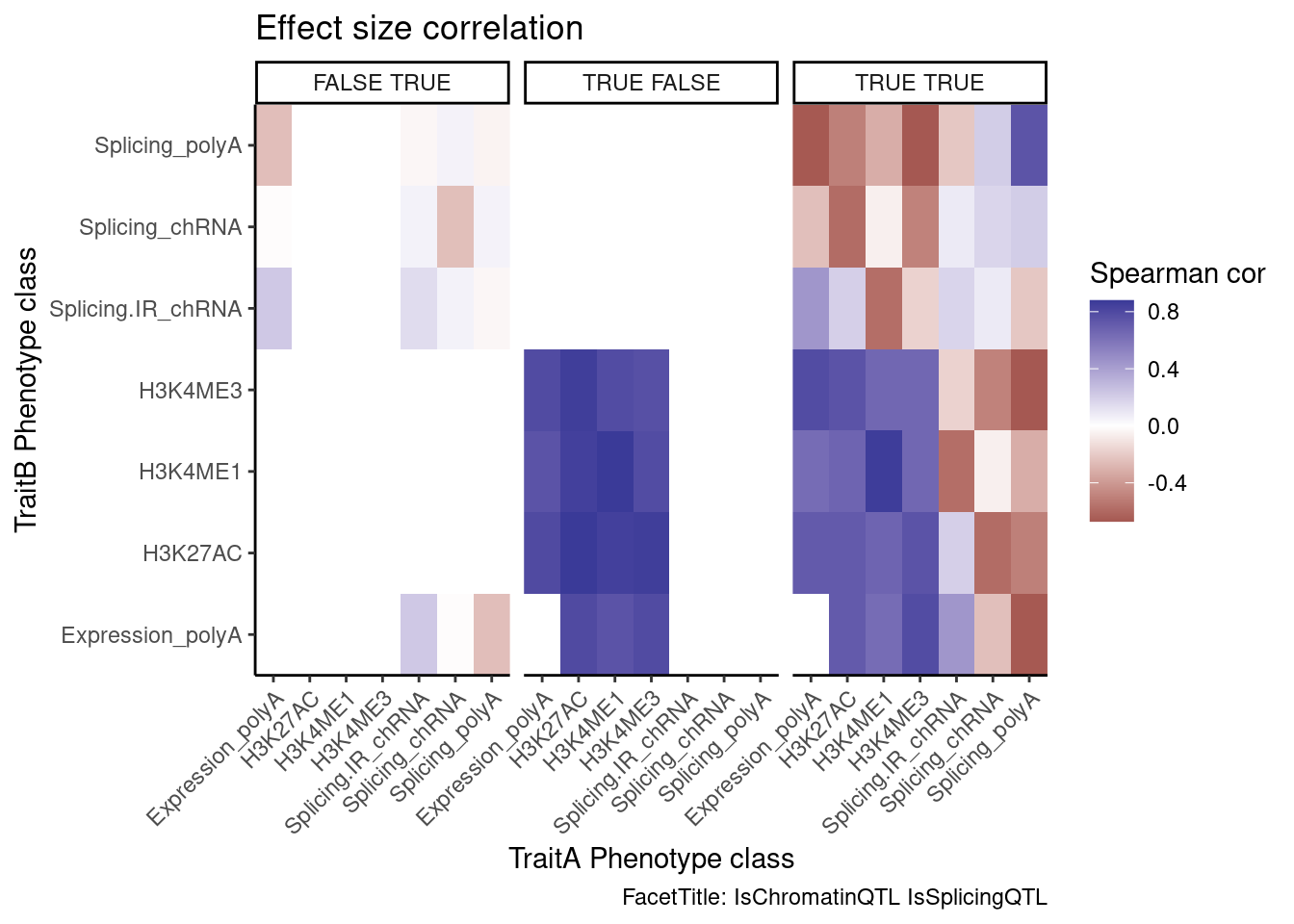
| Version | Author | Date |
|---|---|---|
| 3201a19 | Benjmain Fair | 2022-10-12 |
Now split QTLs by location of SNP as either in splice site, in enhancer/promoter, or neither
#annotation types
finemap.snps.annotated$AnnotationClass %>% unique()
[1] "SpliceBranchpointRegion_0" "10_Txn_Elongation"
[3] "6_Weak_Enhancer" "SpliceDonor_0"
[5] "2_Weak_Promoter" "11_Weak_Txn"
[7] "1_Active_Promoter" "12_Repressed"
[9] "4_Strong_Enhancer" "13_Heterochrom/lo"
[11] "SpliceAcceptor_0" "SpliceBranchpointRegion_1"
[13] "ncRNA_coRNA" "ncRNA_pseudo"
[15] "9_Txn_Transition" "SpliceAcceptor_1"
[17] "ncRNA_srtRNA" "8_Insulator"
[19] "ncRNA_uaRNA" "5_Strong_Enhancer"
[21] "7_Weak_Enhancer" "SpliceDonor_1"
[23] "PAS_Region" "ncRNA_incRNA"
[25] "3_Poised_Promoter" "."
[27] "14_Repetitive/CNV" "ncRNA_ctRNA"
[29] "15_Repetitive/CNV" "ncRNA_lncRNA"
[31] "ncRNA_rtRNA" "ncRNA_snoRNA" coloc.results.tidycolocalized %>%
group_by(Locus, snp) %>%
filter(any(PC=="Expression.Splicing.Subset_YRI")) %>%
ungroup() %>%
filter(PC %in% c("Expression.Splicing.Subset_YRI","H3K27AC", "H3K4ME1", "H3K4ME3", "polyA.Splicing.Subset_YRI", "chRNA.Splicing", "chRNA.IER")) %>%
left_join(., ., by=c("Locus", "snp")) %>%
filter(!((P.x == P.y) & (PC.x == PC.y))) %>%
group_by(Locus, snp) %>%
mutate(
ContainsChromatinEqtl = any(PC.x %in% c("H3K27AC", "H3K4ME1", "H3K4ME3")),
ContainsSqtl = any(PC.x %in% c("polyA.Splicing.Subset_YRI", "chRNA.Splicing", "chRNA.IER"))
) %>%
ungroup() %>%
mutate(Contains.eQTL_Contains.sQTL = paste(ContainsChromatinEqtl, ContainsSqtl)) %>%
dplyr::select(-iteration.y) %>%
left_join(
finemap.snps.annotated %>%
dplyr::select(SNP_iteration_locus, FinemapPP, AnnotationClass) %>%
separate(SNP_iteration_locus, into=c("snp", "iteration.x", "Locus"), convert=T, sep="_")
) %>%
filter(FinemapPP >0.25) %>%
mutate(AnnotationSuperclass = case_when(
str_detect(AnnotationClass, "Splice.+_1") ~ "Annotated SS",
str_detect(AnnotationClass, "Splice.+_0$") ~ "Unannotated SS",
str_detect(AnnotationClass, "Enhancer") ~ "Enhancer",
str_detect(AnnotationClass, "Promoter") ~ "Promoter",
TRUE ~ "Other"
)) %>%
mutate(PC.x = recode(PC.x, !!!PC.ShortAliases)) %>%
mutate(PC.y = recode(PC.y, !!!PC.ShortAliases)) %>%
mutate(Contains.eQTL_Contains.sQTL = recode(Contains.eQTL_Contains.sQTL,
!!!c("TRUE TRUE"="hQTL+sQTL",
"TRUE FALSE"="hQTL only",
"FALSE TRUE"="sQTL only"))) %>%
group_by(Contains.eQTL_Contains.sQTL, PC.x, PC.y, AnnotationSuperclass) %>%
summarise(cor = cor(beta.x, beta.y, method="spearman"), n=n()) %>%
ggplot(aes(x=PC.x, y=PC.y, fill=cor)) +
geom_raster() +
geom_text(aes(label=n), size=1.5) +
scale_fill_gradient2() +
facet_grid(rows=vars(Contains.eQTL_Contains.sQTL), cols=vars(AnnotationSuperclass)) +
scale_x_discrete(expand=c(0,0)) +
scale_y_discrete(expand=c(0,0)) +
theme_classic() +
theme(axis.text.x = element_text(angle = 45, vjust = 1, hjust=1)) +
labs(x="TraitA Phenotype class", y="TraitB Phenotype class", fill="Spearman cor", title="Effect size correlation for eQTLs that coloc with something",
caption = str_wrap("FacetCols=Annotation class of SNP (Onlyfinemap PP >0.25 included). FacetRows=Type of eQTL"))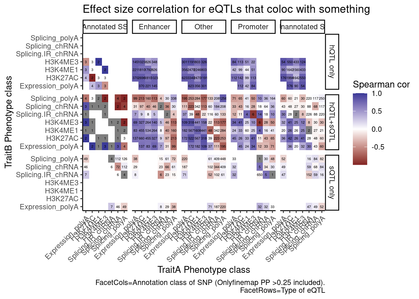
| Version | Author | Date |
|---|---|---|
| 3201a19 | Benjmain Fair | 2022-10-12 |
I’m quite surprised just by the numbers of hQTL eQTLs with high finemap PP in unannoated splice site regions. This is clearly a really big annotation set that also includes lots of enhancer regions. This unannoated splice site region was defined as at least one spliced read mapping across all the data. Perhaps I shouldn’t be surprised, as any region is sufficeintly transcribed (including enhancers) will at some rate have some splice sites.
And even among the 7 intron retention QTLs that coloc with an eQTL but not hQTL, and are finemapped to annotated splice sites, the the direction of effects is if anything opposite what I was expecting
coloc.results.tidycolocalized %>%
  group_by(Locus, snp) %>%
  filter(any(PC=="Expression.Splicing.Subset_YRI")) %>%
  ungroup() %>%
  filter(PC %in% c("Expression.Splicing.Subset_YRI","H3K27AC", "H3K4ME1", "H3K4ME3", "polyA.Splicing.Subset_YRI", "chRNA.Splicing", "chRNA.IER")) %>%
  left_join(., ., by=c("Locus", "snp")) %>%
  filter(!((P.x == P.y) & (PC.x == PC.y))) %>%
  group_by(Locus, snp) %>%
  mutate(
    ContainsChromatinEqtl = any(PC.x %in% c("H3K27AC", "H3K4ME1", "H3K4ME3")),
    ContainsSqtl = any(PC.x %in% c("polyA.Splicing.Subset_YRI", "chRNA.Splicing", "chRNA.IER"))
    ) %>%
  ungroup() %>%
  mutate(Contains.eQTL_Contains.sQTL = paste(ContainsChromatinEqtl, ContainsSqtl)) %>%
  dplyr::select(-iteration.y) %>%
  left_join(
    finemap.snps.annotated %>%
      dplyr::select(SNP_iteration_locus, FinemapPP, AnnotationClass) %>%
      separate(SNP_iteration_locus, into=c("snp", "iteration.x", "Locus"), convert=T, sep="_")
  ) %>%
  filter(FinemapPP >0.25) %>%
  mutate(AnnotationSuperclass = case_when(
    str_detect(AnnotationClass, "Splice.+_1") ~ "Annotated SS",
    str_detect(AnnotationClass, "Splice.+_0$") ~ "Unannotated SS",
    str_detect(AnnotationClass, "Enhancer") ~ "Enhancer",
    str_detect(AnnotationClass, "Promoter") ~ "Promoter",
    TRUE ~ "Other"
  )) %>%
  mutate(PC.x = recode(PC.x, !!!PC.ShortAliases)) %>%
  mutate(PC.y = recode(PC.y, !!!PC.ShortAliases)) %>%
  mutate(Contains.eQTL_Contains.sQTL = recode(Contains.eQTL_Contains.sQTL,
                                              !!!c("TRUE TRUE"="hQTL+sQTL",
                                                   "TRUE FALSE"="hQTL only",
                                                   "FALSE TRUE"="sQTL only"))) %>%
  filter(Contains.eQTL_Contains.sQTL=="sQTL only" & AnnotationSuperclass=="Annotated SS") %>%
  ggplot(aes(x=beta.x, y=beta.y)) +
  geom_point() +
  geom_vline(xintercept=0) +
  geom_hline(yintercept=0) +
  facet_grid(rows=vars(PC.x), cols=vars(PC.y)) +
  theme_bw() +
  labs(x="TraitA Phenotype class", y="TraitB Phenotype class", title="Effect size correlation for eQTLs/sQTLs that are not hQTLs",
       caption = str_wrap("Only SNPs with finemap PP > 0.25 in annotated splice site SNP included"))
| Version | Author | Date |
|---|---|---|
| 3201a19 | Benjmain Fair | 2022-10-12 |
Note there are only a few points of chRNA.IR intron retention with SNPs in splice sites that coloc with eQTL.
Let’s check how these plots look for NMD-specific introns…
dat.to.plot <- coloc.results.tidycolocalized %>%
  group_by(Locus, snp) %>%
  filter(any(PC=="Expression.Splicing.Subset_YRI")) %>%
  ungroup() %>%
  filter(PC %in% c("Expression.Splicing.Subset_YRI","H3K27AC", "H3K4ME1", "H3K4ME3", "polyA.Splicing.Subset_YRI", "chRNA.Splicing", "chRNA.IER")) %>%
  left_join(., ., by=c("Locus", "snp")) %>%
  filter(!((P.x == P.y) & (PC.x == PC.y))) %>%
  group_by(Locus, snp) %>%
  mutate(
    ContainsChromatinEqtl = any(PC.x %in% c("H3K27AC", "H3K4ME1", "H3K4ME3")),
    ContainsSqtl = any(PC.x %in% c("polyA.Splicing.Subset_YRI", "chRNA.Splicing", "chRNA.IER"))
    ) %>%
  ungroup() %>%
  mutate(Contains.eQTL_Contains.sQTL = paste(ContainsChromatinEqtl, ContainsSqtl)) %>%
  dplyr::select(-iteration.y) %>%
  left_join(
    finemap.snps.annotated %>%
      dplyr::select(SNP_iteration_locus, FinemapPP, AnnotationClass) %>%
      separate(SNP_iteration_locus, into=c("snp", "iteration.x", "Locus"), convert=T, sep="_")
  ) %>%
  filter(FinemapPP >0.25) %>%
  mutate(AnnotationSuperclass = case_when(
    str_detect(AnnotationClass, "Splice.+_1") ~ "Annotated SS",
    str_detect(AnnotationClass, "Splice.+_0$") ~ "Unannotated SS",
    str_detect(AnnotationClass, "Enhancer") ~ "Enhancer",
    str_detect(AnnotationClass, "Promoter") ~ "Promoter",
    TRUE ~ "Other"
  )) %>%
  mutate(PC.x = recode(PC.x, !!!PC.ShortAliases)) %>%
  mutate(PC.y = recode(PC.y, !!!PC.ShortAliases)) %>%
  mutate(Contains.eQTL_Contains.sQTL = recode(Contains.eQTL_Contains.sQTL,
                                              !!!c("TRUE TRUE"="hQTL+sQTL",
                                                   "TRUE FALSE"="hQTL only",
                                                   "FALSE TRUE"="sQTL only"))) %>%
  filter(Contains.eQTL_Contains.sQTL=="sQTL only") %>%
  mutate(New.x = str_replace(P.x, "^(.+?):(.+?):(.+?):.+?_([-+])$", "chr\\1_\\2_\\3_\\4")) %>%
  mutate(New.y = str_replace(P.x, "^(.+?):(.+?):(.+?):.+?_([-+])$", "chr\\1_\\2_\\3_\\4")) %>%
  mutate(ContainsNMDJunc = (New.x %in% NMD.specific.introns) | (New.y %in% NMD.specific.introns)) %>%
  arrange(ContainsNMDJunc)
ggplot(dat.to.plot, aes(x=beta.x, y=beta.y, color=ContainsNMDJunc)) +
  geom_point(alpha=0.5) +
  geom_vline(xintercept=0) +
  geom_hline(yintercept=0) +
  geom_smooth(method='lm') +
  facet_grid(rows=vars(PC.x), cols=vars(PC.y)) +
  theme_bw() +
  labs(x="TraitA Phenotype class", y="TraitB Phenotype class", caption="Effect size correlation for eQTLs/sQTLs that are not hQTLs", title="sQTLs that increase annotated NMD junctions coloc with downward eQTLs")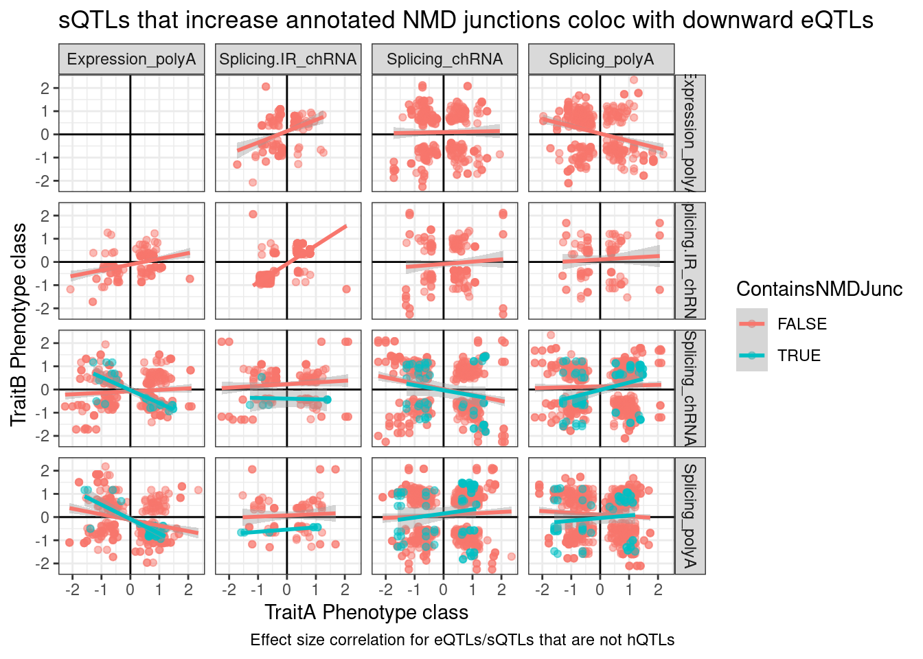
| Version | Author | Date |
|---|---|---|
| 3201a19 | Benjmain Fair | 2022-10-12 |
So there’s clearly a negative correlation between NMD-specific intron splicing and expression. But there’s only so many NMD introns annotated, and I expect a lot of splice changes due to genetic variation to be unannotated. Additionally, a lot of the red dots might the necessary down-regulated junctions when a NMD-junction gets up-regulated.
Let’s plot all the blue points with pygenometracks
dir.create("../code/scratch/PlotNMDsQTLeQTLs/")

dat.to.plot.filtered <- dat.to.plot %>%
  filter(ContainsNMDJunc) %>%
  filter(PC.y %in% "Expression_polyA") %>%
  distinct(Locus, .keep_all=T)

#Write out all juncs in clusters
dat.to.plot.filtered %>%
  mutate(gid = str_replace(P.x, "^(.+?):.+?:.+?:(.+?)", "chr\\1_\\2")) %>%
  inner_join(
    SpliceJunctionCountTables$Expression.Splicing %>% dplyr::select(junc, gid)
  ) %>%
  dplyr::select(junc) %>%
  separate(junc, into=c("chrom", "start", "stop", "name"), sep=":", convert=T) %>%
  arrange(chrom, start, stop) %>%
  write_tsv("../code/scratch/PlotNMDsQTLeQTLs/.juncs.bed")

# # Write out NMD introns
# dat.to.plot.filtered %>%
#   dplyr::select(junc = P.x) %>%
#   separate(junc, into=c("chrom", "start", "stop", "name"), sep=":", convert=T) %>%
#   mutate(chrom=paste0("chr", chrom)) %>%
#   dplyr::select(chrom, start=newstart, stop) %>%
#   arrange(chrom, start, stop) %>%
#   write_tsv("../code/scratch/PlotNMDsQTLeQTLs/.NMD.introns.bed", col_names = F)
#
# # Write out ini file for NMD introns track
# fileConn<-file("../code/scratch/PlotNMDsQTLeQTLs/.NMD.introns.ini")
# writeLines(c("[NMD.introns]","file_type = bed", "type = vlines", "color=red","file = scratch/PlotNMDsQTLeQTLs/.NMD.introns.bed"), con=fileConn)
# close(fileConn)

# Write out NMD introns
dat.to.plot.filtered %>%
  dplyr::select(junc = P.x) %>%
  separate(junc, into=c("chrom", "start", "stop", "name"), sep=":", convert=T) %>%
  mutate(chrom=paste0("chr", chrom)) %>%
  arrange(chrom, start, stop) %>%
  write_tsv("../code/scratch/PlotNMDsQTLeQTLs/.NMD.introns.bed", col_names = F)

# Write out ini file for NMD introns track
fileConn<-file("../code/scratch/PlotNMDsQTLeQTLs/.NMD.introns.ini")
writeLines(c("[NMD.introns]","file_type = bed", "color=red","file = scratch/PlotNMDsQTLeQTLs/.NMD.introns.bed"), con=fileConn)
close(fileConn)

# Write out bash script
dat.to.plot.filtered %>%
  separate(P.x, into=c("chrom", "start", "stop", "name"), sep=":", convert=T) %>%
  mutate(chrom=paste0("chr", chrom)) %>%
  mutate(min=start-10000, max=stop+10000) %>%
  mutate(SnpPos = str_replace(snp, "^(.+?:.+?):.+?:.+?$", "chr\\1")) %>%
  mutate(rn = str_pad(row_number(), 2, pad=0)) %>%
  mutate(cmd = str_glue("python scripts/GenometracksByGenotype/AggregateBigwigsForPlotting.py --VCF Genotypes/1KG_GRCh38/Autosomes.vcf.gz --SnpPos {SnpPos} --GroupSettingsFile Metaplots/bwGroups.tsv --BigwigList Metaplots/bwList.tsv --Normalization WholeGenome --Region {chrom}:{min}-{max} --BigwigListType KeyFile --OutputPrefix scratch/PlotNMDsQTLeQTLs/. -v --Bed12GenesToIni scripts/GenometracksByGenotype/PremadeTracks/gencode.v26.FromGTEx.genes.bed12.gz  --FilterJuncsByBed scratch/PlotNMDsQTLeQTLs/.juncs.bed\npyGenomeTracks --tracks <(cat scratch/PlotNMDsQTLeQTLs/.tracks.ini scratch/PlotNMDsQTLeQTLs/.NMD.introns.ini) --out scratch/PlotNMDsQTLeQTLs/Plot_{rn}_{Locus}.pdf --region {chrom}:{min}-{max} --trackLabelFraction 0.15\n\n")) %>%
  select(cmd) %>%
  write.table("../code/scratch/PlotNMDsQTLeQTLs/MakePlots.sh", quote=F, row.names = F, col.names = F)
..And plot them
conda activate GenometracksByGenotype
cd /project2/yangili1/bjf79/ChromatinSplicingQTLs/code
bash scratch/PlotNMDsQTLeQTLs/MakePlots.sh
And Let’s also expand these results by taking all NMD sQTLs and consider the beta on gene expression…
sQTLs <- c("../code/QTLs/QTLTools/polyA.Splicing.Subset_YRI/PermutationPassForColoc.txt.gz", "../code/QTLs/QTLTools/chRNA.Splicing/PermutationPassForColoc.txt.gz") %>%
  setNames(str_replace(., "../code/QTLs/QTLTools/(.+?)/PermutationPassForColoc.txt.gz", "\\1")) %>%
  lapply(fread) %>%
  bind_rows(.id="source") %>%
  mutate(gene = str_replace(phe_id, ".+:(EN.+?)$", "\\1")) %>%
  mutate(intron = str_replace(phe_id, "^(.+):(.+?):(.+?):clu.+?_([+-]):EN.+$", "chr\\1_\\2_\\3_\\4")) %>%
  group_by(source) %>%
  mutate(q = qvalue(adj_emp_pval)$qvalues) %>%
  ungroup()


eQTLs <- c("../code/QTLs/QTLTools/Expression.Splicing.Subset_YRI/PermutationPassForColoc.txt.gz", "../code/QTLs/QTLTools/chRNA.Expression.Splicing/PermutationPassForColoc.txt.gz") %>%
  setNames(str_replace(., "../code/QTLs/QTLTools/(.+?)/PermutationPassForColoc.txt.gz", "\\1")) %>%
  lapply(fread) %>%
  bind_rows(.id="source") %>%
  mutate(gene = str_replace(phe_id, ".+:(EN.+?)$", "\\1")) %>%
  group_by(source) %>%
  mutate(q = qvalue(adj_emp_pval)$qvalues) %>%
  ungroup()

H3K4me3.QTLs <- c("../code/QTLs/QTLTools/H3K4ME3/PermutationPassForColoc.txt.gz") %>%
  setNames(str_replace(., "../code/QTLs/QTLTools/(.+?)/PermutationPassForColoc.txt.gz", "\\1")) %>%
  lapply(fread) %>%
  bind_rows(.id="source") %>%
  mutate(gene = str_replace(phe_id, ".+:(EN.+?)$", "\\1")) %>%
  mutate(gene_peak = str_replace(phe_id, "^(.+?):(.+?)$", "\\2;\\1")) %>%
  group_by(source) %>%
  mutate(q = qvalue(adj_emp_pval)$qvalues) %>%
  ungroup()

PeaksToTSS <- Sys.glob("../code/Misc/PeaksClosestToTSS/*_assigned.tsv.gz") %>%
  setNames(str_replace(., "../code/Misc/PeaksClosestToTSS/(.+?)_assigned.tsv.gz", "\\1")) %>%
  lapply(read_tsv) %>%
  bind_rows(.id="ChromatinMark") %>%
  mutate(GenePeakPair = paste(gene, peak, sep = ";")) %>%
  distinct(ChromatinMark, peak, gene, .keep_all=T)

inner_join(eQTLs, sQTLs, by="gene", suffix=c(".eQTL", ".sQTL")) %>%
  mutate(Is.NMD.intron = intron %in% NMD.specific.introns) %>%
  filter(q.eQTL < 0.1 & q.sQTL < 0.1) %>%
  mutate(source.eQTL = recode(source.eQTL, !!!c("polyA.Expression.YRI"="Expression.Splicing.Subset_YRI", "chRNA.Expression"="chRNA.Expression.Splicing"))) %>%
  arrange(Is.NMD.intron) %>%
  ggplot(aes(x=slope.eQTL, y=slope.sQTL, color=Is.NMD.intron)) +
  geom_point(alpha=0.5) +
  geom_vline(xintercept=0) +
  geom_hline(yintercept=0) +
  geom_smooth(method='lm') +
  facet_grid(rows = vars(source.eQTL), cols=vars(source.sQTL)) +
  theme_bw() +
  labs(title="genetic effects of NMD introns and host gene expression", x="beta, eQTL", y="beta, sQTL", caption="Only FDR<10% sQTLs and eQTLs plotted")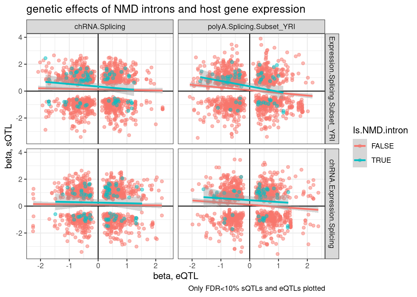
inner_join(eQTLs, H3K4me3.QTLs, by="gene", suffix=c(".eQTL", ".sQTL")) %>%
  filter(gene_peak %in% PeaksToTSS$GenePeakPair) %>%
  filter(q.eQTL < 0.1 & q.sQTL < 0.1) %>%
  mutate(source.eQTL = recode(source.eQTL, !!!c("polyA.Expression.YRI"="Expression.Splicing.Subset_YRI", "chRNA.Expression"="chRNA.Expression.Splicing"))) %>%
  ggplot(aes(x=slope.eQTL, y=slope.sQTL)) +
  geom_point(alpha=0.5) +
  geom_vline(xintercept=0) +
  geom_hline(yintercept=0) +
  geom_smooth(method='lm') +
  facet_grid(rows = vars(source.eQTL), cols=vars(source.sQTL)) +
  theme_bw() +
  labs(title="genetic effects of H3K4ME promoters and host gene expression", x="beta, eQTL", y="beta, H3K4ME3 QTL", caption="Only FDR<10% H3K4ME3 QTLs and eQTLs plotted")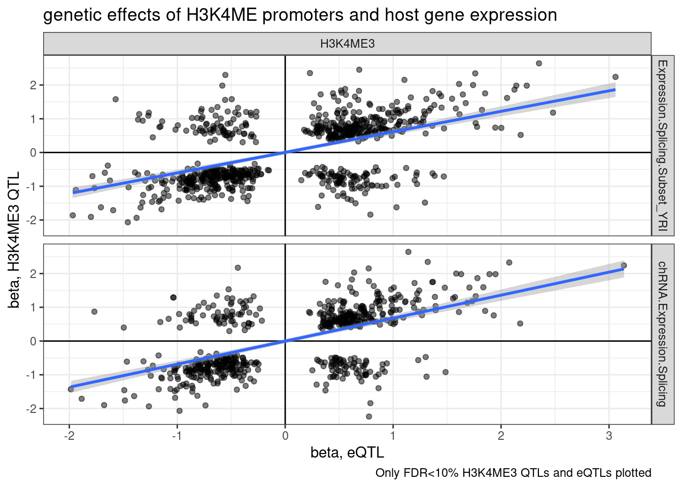
Wait, upon further thought, I think I didn’t make the above plots correctly. I was just plotting the beta for the topSNP for each feature, not the same SNP between sQTL and eQTL, so the directions of SNP effect (which are always ALT/REF) might not be polarized the same way.
TopSNPEffects.ByPairs <- fread("../code/pi1/PairwisePi1Traits.P.all.txt.gz")

TopSNPEffects.ByPairs %>%
  filter(
      (PC1 %in% c("chRNA.Expression.Splicing", "Expression.Splicing.Subset_YRI")) &
      (PC2 %in% c("polyA.Splicing.Subset_YRI", "chRNA.Splicing")) &
      (FDR.x < 0.1) &
      (FDR.y < 0.1)) %>%
  mutate(source.eQTL = recode(PC1, !!!c("Expression.Splicing.Subset_YRI"="polyA.Expression.YRI", "chRNA.Expression.Splicing"="chRNA.Expression"))) %>%
  rename(source.sQTL=PC2) %>%
  mutate(intron = str_replace(P2, "^(.+):(.+?):(.+?):clu.+?_([+-])$", "chr\\1_\\2_\\3_\\4")) %>%
  mutate(Is.NMD.intron = intron %in% NMD.specific.introns) %>%
  arrange(Is.NMD.intron) %>%
  ggplot(aes(x=beta.x, y=trait.x.beta.in.y
, color=Is.NMD.intron)) +
  geom_point(alpha=0.5) +
  geom_vline(xintercept=0) +
  geom_hline(yintercept=0) +
  geom_smooth(method='lm') +
  facet_grid(rows = vars(source.eQTL), cols=vars(source.sQTL)) +
  theme_bw() +
  labs(title="genetic effects of NMD introns and host gene expression", x="beta, eQTL", y="beta, sQTL", caption="Only FDR<10% sQTLs and eQTLs plotted. sQTL effects are relative to top eQTL SNP")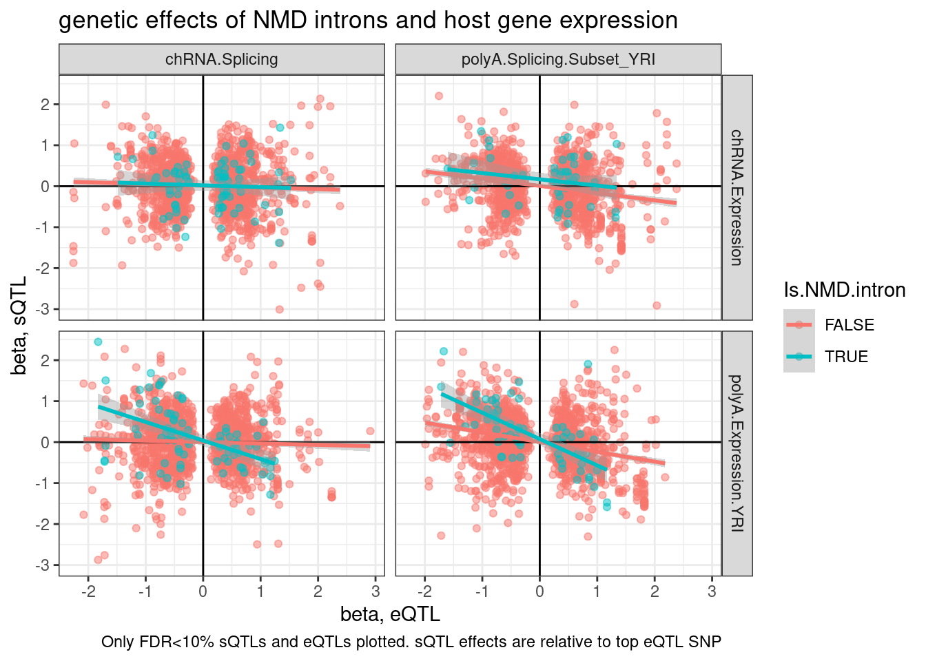
TopSNPEffects.ByPairs %>%
filter(
(PC2 %in% c("chRNA.Expression.Splicing", "Expression.Splicing.Subset_YRI")) &
(PC1 %in% c("polyA.Splicing.Subset_YRI", "chRNA.Splicing")) &
(FDR.x < 0.1) &
(FDR.y < 0.1)) %>%
mutate(source.eQTL = recode(PC2, !!!c("Expression.Splicing.Subset_YRI"="polyA.Expression.YRI", "chRNA.Expression.Splicing"="chRNA.Expression"))) %>%
rename(source.sQTL=PC1) %>%
mutate(intron = str_replace(P1, "^(.+):(.+?):(.+?):clu.+?_([+-])$", "chr\\1_\\2_\\3_\\4")) %>%
mutate(Is.NMD.intron = intron %in% NMD.specific.introns) %>%
arrange(Is.NMD.intron) %>%
ggplot(aes(y=beta.x, x=trait.x.beta.in.y
, color=Is.NMD.intron)) +
geom_point(alpha=0.5) +
geom_vline(xintercept=0) +
geom_hline(yintercept=0) +
geom_smooth(method='lm') +
facet_grid(rows = vars(source.eQTL), cols=vars(source.sQTL)) +
theme_bw() +
labs(title="genetic effects of NMD introns and host gene expression", x="beta, eQTL", y="beta, sQTL", caption="Only FDR<10% sQTLs and eQTLs plotted. eQTL effects are relative to top sQTL SNP")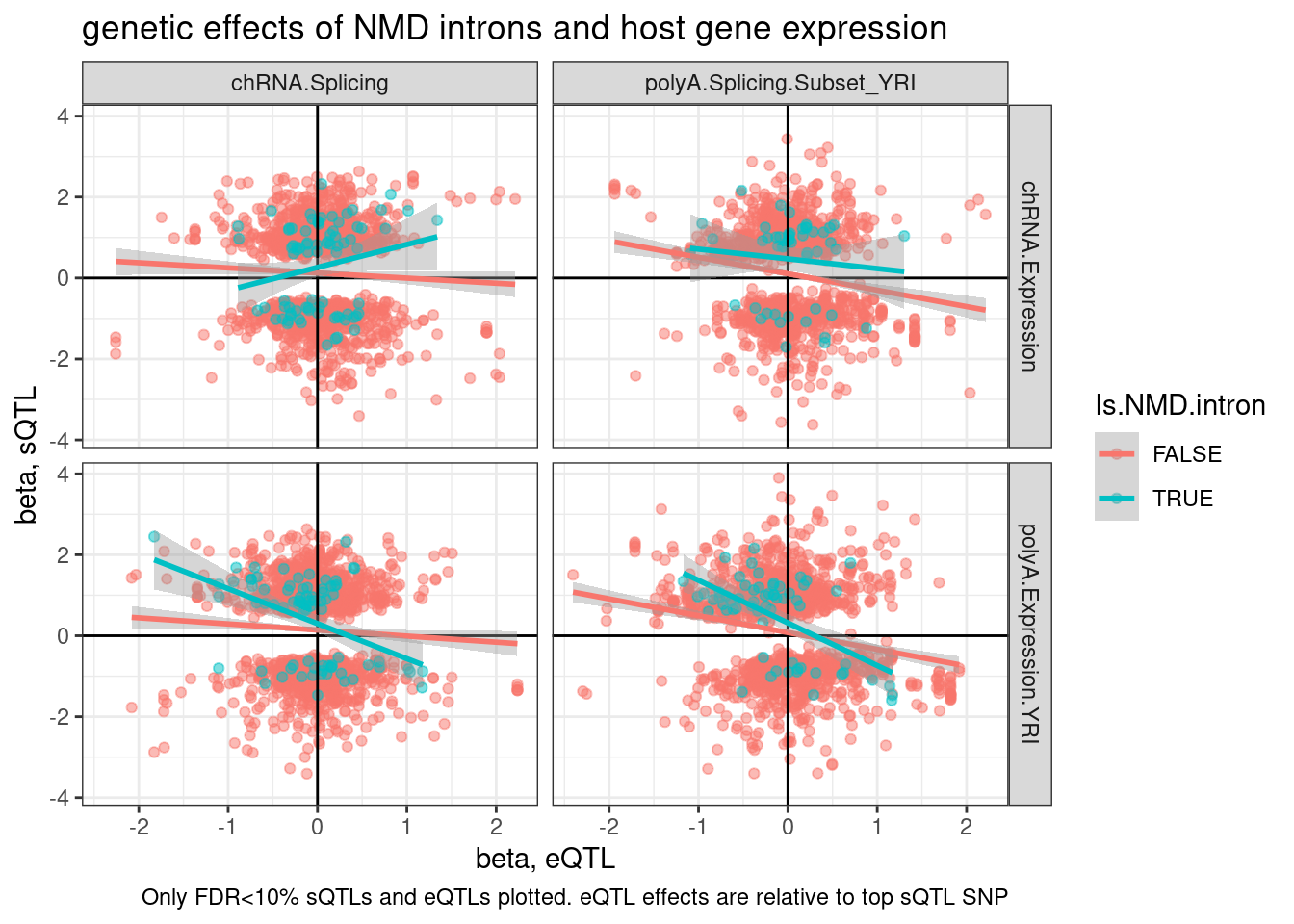 I think I’ll want to further break down introns into - annotatic basic transcripts - annotated transripts (not NMD) - annotated NMD - unannotated
First read in the annotations…
Intron.Annotations.basic <- read_tsv("../code/SplicingAnalysis/regtools_annotate_combined/basic.bed.gz") %>%
  filter(known_junction ==1) %>%
  unite(intron, chrom, start, end, strand)
Introns.Annotations.comprehensive <- read_tsv("../code/SplicingAnalysis/regtools_annotate_combined/comprehensive.bed.gz") %>%
  filter(known_junction ==1) %>%
  unite(intron, chrom, start, end, strand)
Now remake the plots
TopSNPEffects.ByPairs %>%
  filter(
      (PC1 %in% c("chRNA.Expression.Splicing", "Expression.Splicing.Subset_YRI")) &
      (PC2 %in% c("polyA.Splicing.Subset_YRI", "chRNA.Splicing")) &
      (FDR.x < 0.1) &
      (FDR.y < 0.1)) %>%
  mutate(source.eQTL = recode(PC1, !!!c("Expression.Splicing.Subset_YRI"="polyA.Expression.YRI", "chRNA.Expression.Splicing"="chRNA.Expression"))) %>%
  rename(source.sQTL=PC2) %>%
  mutate(intron = str_replace(P2, "^(.+):(.+?):(.+?):clu.+?_([+-])$", "chr\\1_\\2_\\3_\\4")) %>%
  mutate(IntronAnnotation = case_when(
    intron %in% NMD.specific.introns ~ "Annotated NMD",
    intron %in% Intron.Annotations.basic$intron ~ "Annotated basic",
    intron %in% Introns.Annotations.comprehensive$intron ~ "Annotated Not basic",
    TRUE ~ "Unannotated"
  )) %>%
  count(IntronAnnotation) %>%
  ggplot(aes(x=IntronAnnotation, y=n, fill=IntronAnnotation)) +
  geom_col() +
  theme_bw() +
  theme(axis.text.x = element_text(angle = 45, vjust = 1, hjust=1)) +
  labs(title="Number sQTLs that are in an eGene", x="Intron Type", caption="FDR10% for sQTL and eQTL")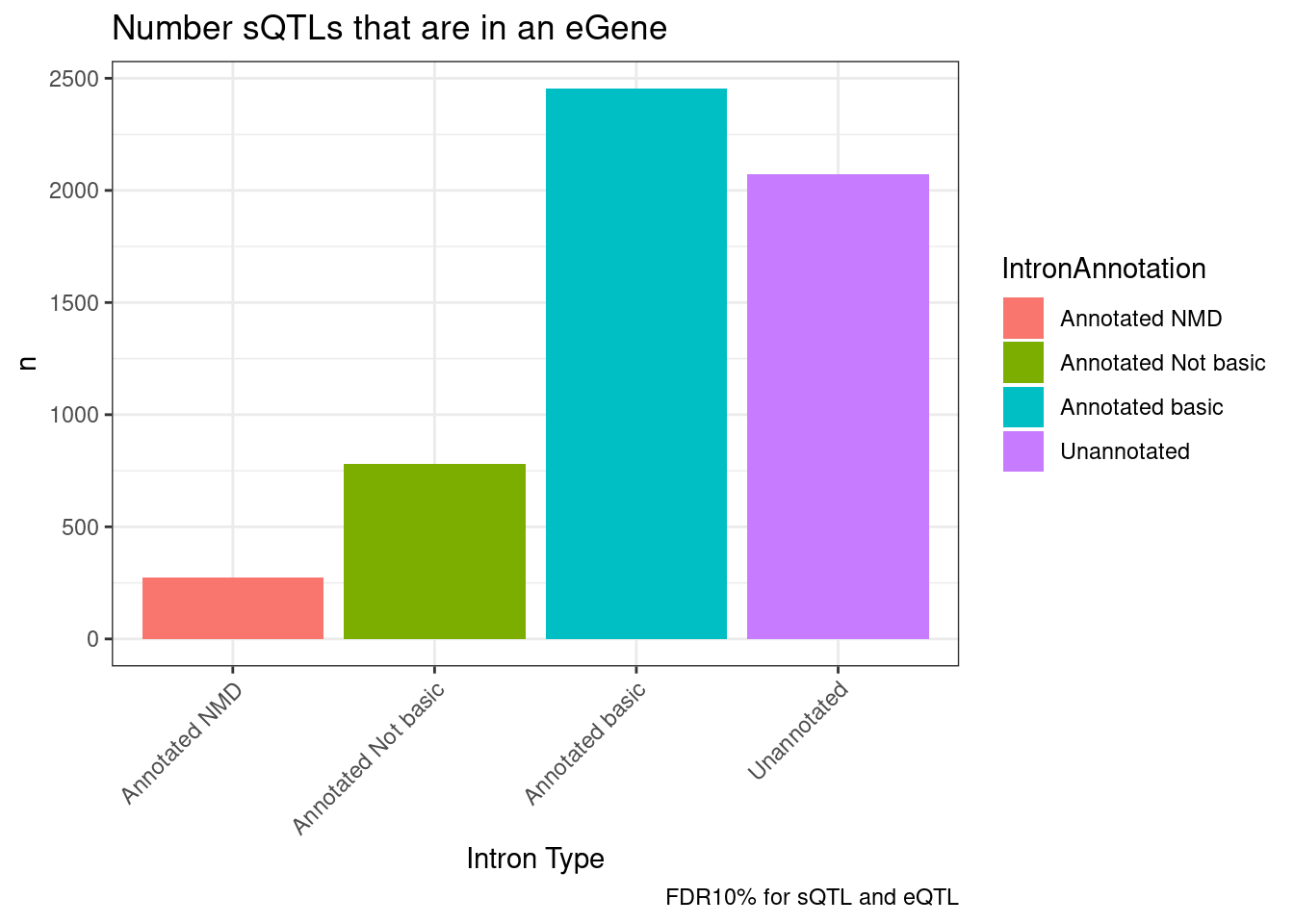
TopSNPEffects.ByPairs %>%
  filter(
      (PC1 %in% c("chRNA.Expression.Splicing", "Expression.Splicing.Subset_YRI")) &
      (PC2 %in% c("polyA.Splicing.Subset_YRI", "chRNA.Splicing")) &
      (FDR.x < 0.1) &
      (FDR.y < 0.1)) %>%
  mutate(source.eQTL = recode(PC1, !!!c("Expression.Splicing.Subset_YRI"="polyA.Expression.YRI", "chRNA.Expression.Splicing"="chRNA.Expression"))) %>%
  rename(source.sQTL=PC2) %>%
  mutate(intron = str_replace(P2, "^(.+):(.+?):(.+?):clu.+?_([+-])$", "chr\\1_\\2_\\3_\\4")) %>%
  mutate(IntronAnnotation = case_when(
    intron %in% NMD.specific.introns ~ "Annotated NMD",
    intron %in% Intron.Annotations.basic$intron ~ "Annotated basic",
    intron %in% Introns.Annotations.comprehensive$intron ~ "Annotated Not basic",
    TRUE ~ "Unannotated"
  )) %>%
  ggplot(aes(y=beta.x, x=trait.x.beta.in.y
, color=IntronAnnotation)) +
  geom_point(alpha=0.5) +
  geom_vline(xintercept=0) +
  geom_hline(yintercept=0) +
  geom_smooth(method='lm') +
  facet_grid(rows = vars(source.eQTL), cols=vars(source.sQTL)) +
  theme_bw() +
  labs(title="genetic effects of NMD introns and host gene expression", x="beta, sQTL", y="beta, eQTL", caption="Only FDR<10% sQTLs and eQTLs plotted. sQTL effects are relative to top eQTL SNP")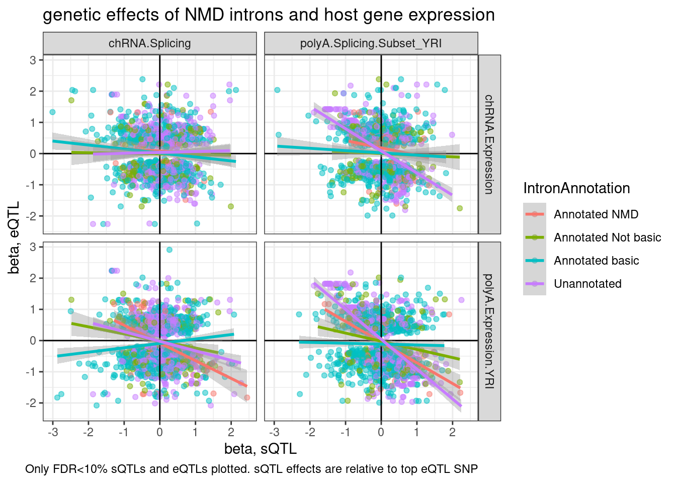
TopSNPEffects.ByPairs %>%
  filter(
      (PC2 %in% c("chRNA.Expression.Splicing", "Expression.Splicing.Subset_YRI")) &
      (PC1 %in% c("polyA.Splicing.Subset_YRI", "chRNA.Splicing")) &
      (FDR.x < 0.1) &
      (FDR.y < 0.1)) %>%
  mutate(source.eQTL = recode(PC2, !!!c("Expression.Splicing.Subset_YRI"="polyA.Expression.YRI", "chRNA.Expression.Splicing"="chRNA.Expression"))) %>%
  rename(source.sQTL=PC1) %>%
  mutate(intron = str_replace(P1, "^(.+):(.+?):(.+?):clu.+?_([+-])$", "chr\\1_\\2_\\3_\\4")) %>%
  mutate(IntronAnnotation = case_when(
    intron %in% NMD.specific.introns ~ "Annotated NMD",
    intron %in% Intron.Annotations.basic$intron ~ "Annotated basic",
    intron %in% Introns.Annotations.comprehensive$intron ~ "Annotated Not basic",
    TRUE ~ "Unannotated"
  )) %>%
  ggplot(aes(y=beta.x, x=trait.x.beta.in.y
, color=IntronAnnotation)) +
  geom_point(alpha=0.5) +
  geom_vline(xintercept=0) +
  geom_hline(yintercept=0) +
  geom_smooth(method='lm') +
  facet_grid(rows = vars(source.eQTL), cols=vars(source.sQTL)) +
  theme_bw() +
  labs(title="genetic effects of NMD introns and host gene expression", x="beta, sQTL", y="beta, eQTL", caption="Only FDR<10% sQTLs and eQTLs plotted. eQTL effects are relative to top sQTL SNP")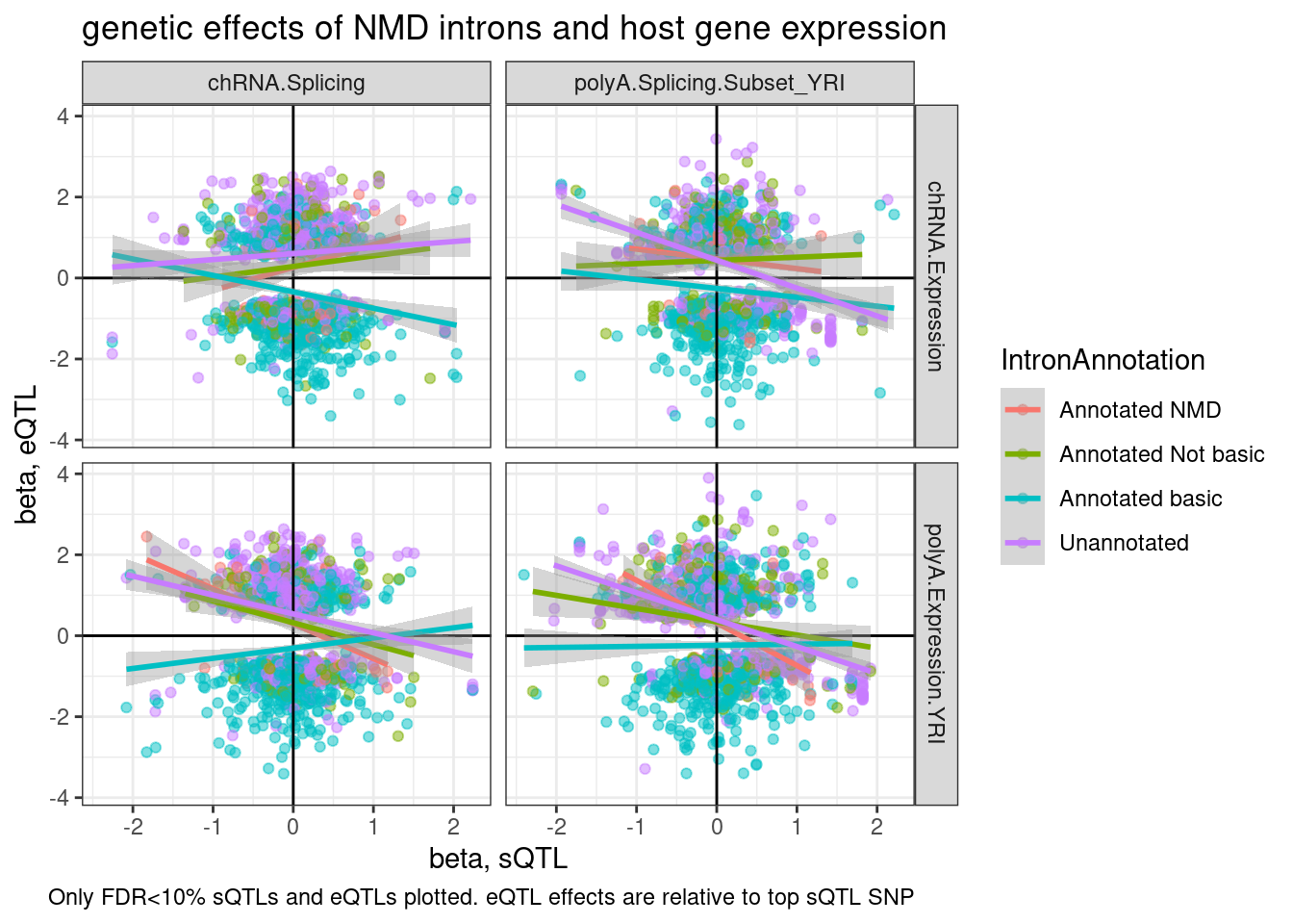
enrichment of NMD sQTLs in eQTLs
Another way to show this, which would look more significant I think is to ask what % of non-eQTL sQTL affect NMD junctions of all non-eQTL sQTLs versus the same for sQTLs that are eQTLs
TopSNPEffects.ByPairs %>%
  filter(
      (PC1 %in% c("chRNA.Expression.Splicing", "Expression.Splicing.Subset_YRI"))) %>%
  # filter(
  #     (PC2 %in% c("chRNA.Expression.Splicing", "Expression.Splicing.Subset_YRI")) &
  #     (PC1 %in% c("polyA.Splicing.Subset_YRI", "chRNA.Splicing")) ) %>%
  filter(FDR.x < 0.1) %>%
  distinct(P1) %>% nrow()
[1] 5358TopSNPEffects.ByPairs %>%
filter(
(PC1 %in% c("polyA.Splicing.Subset_YRI", "chRNA.Splicing")) ) %>%
distinct(GeneLocus) %>% nrow()[1] 2621datToPlot <- TopSNPEffects.ByPairs %>%
filter(
(PC2 %in% c("chRNA.Expression.Splicing", "Expression.Splicing.Subset_YRI")) &
(PC1 %in% c("polyA.Splicing.Subset_YRI", "chRNA.Splicing")) ) %>%
filter(FDR.x < 0.1) %>%
mutate(intron = str_replace(P1, "^(.+):(.+?):(.+?):clu.+?_([+-])$", "chr\\1_\\2_\\3_\\4")) %>%
mutate(IntronAnnotation = case_when(
intron %in% NMD.specific.introns ~ "Annotated NMD",
intron %in% Intron.Annotations.basic$intron ~ "Annotated basic",
intron %in% Introns.Annotations.comprehensive$intron ~ "Annotated Not basic",
TRUE ~ "Unannotated"
)) %>%
mutate(Is_HostGene_eQTL = if_else(FDR.y < 0.1, "eGene", "not eGene")) %>%
count(IntronAnnotation, Is_HostGene_eQTL) %>%
group_by(Is_HostGene_eQTL) %>%
mutate(Percent = n/sum(n)*100) %>%
mutate(rn = row_number()) %>%
ungroup()
ggplot(datToPlot, aes(x=Is_HostGene_eQTL, y=n, fill=IntronAnnotation)) +
geom_col(position="stack") +
geom_label(aes(label=signif(Percent, 3), vjust=rn), y=Inf) +
theme_bw() +
labs(y="Number sQTLs", caption="1406 eGenes identified in YRI with a test intron")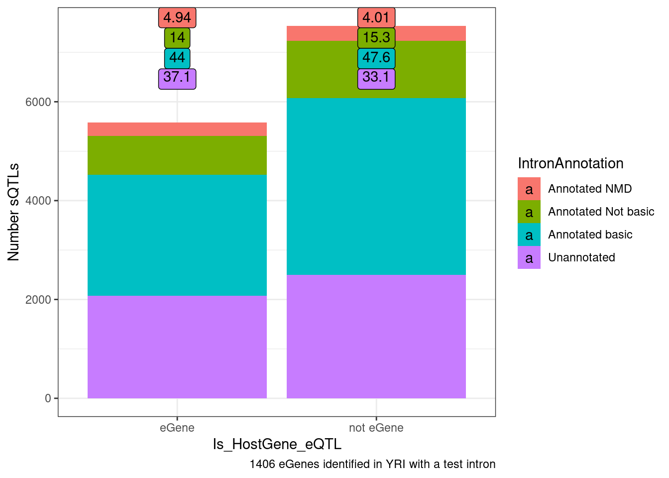
Let’s also break the original plot by ncRNAs for SNP regions
coloc.results.tidycolocalized %>%
  group_by(Locus, snp) %>%
  filter(any(PC=="Expression.Splicing.Subset_YRI")) %>%
  ungroup() %>%
  filter(PC %in% c("Expression.Splicing.Subset_YRI","H3K27AC", "H3K4ME1", "H3K4ME3", "polyA.Splicing.Subset_YRI", "chRNA.Splicing", "chRNA.IER")) %>%
  left_join(., ., by=c("Locus", "snp")) %>%
  filter(!((P.x == P.y) & (PC.x == PC.y))) %>%
  group_by(Locus, snp) %>%
  mutate(
    ContainsChromatinEqtl = any(PC.x %in% c("H3K27AC", "H3K4ME1", "H3K4ME3")),
    ContainsSqtl = any(PC.x %in% c("polyA.Splicing.Subset_YRI", "chRNA.Splicing", "chRNA.IER"))
    ) %>%
  ungroup() %>%
  mutate(Contains.eQTL_Contains.sQTL = paste(ContainsChromatinEqtl, ContainsSqtl)) %>%
  dplyr::select(-iteration.y) %>%
  left_join(
    finemap.snps.annotated %>%
      dplyr::select(SNP_iteration_locus, FinemapPP, AnnotationClass) %>%
      separate(SNP_iteration_locus, into=c("snp", "iteration.x", "Locus"), convert=T, sep="_")
  ) %>%
  filter(FinemapPP >0.25) %>%
  mutate(AnnotationSuperclass = case_when(
    str_detect(AnnotationClass, "Splice.+_1") ~ "Annotated SS",
    str_detect(AnnotationClass, "Splice.+_0$") ~ "Unannotated SS",
    str_detect(AnnotationClass, "Enhancer") ~ "Enhancer",
    str_detect(AnnotationClass, "Promoter") ~ "Promoter",
    str_detect(AnnotationClass, "ncRNA") ~ AnnotationClass,
    TRUE ~ "Other"
  )) %>%
  group_by(Contains.eQTL_Contains.sQTL, PC.x, PC.y, AnnotationSuperclass) %>%
  summarise(cor = cor(beta.x, beta.y, method="spearman"), n=n()) %>%
  mutate(PC.x = recode(PC.x, !!!PC.ShortAliases)) %>%
  mutate(PC.y = recode(PC.y, !!!PC.ShortAliases)) %>%
  mutate(Contains.eQTL_Contains.sQTL = recode(Contains.eQTL_Contains.sQTL,
                                              !!!c("TRUE TRUE"="hQTL+sQTL",
                                                   "TRUE FALSE"="hQTL only",
                                                   "FALSE TRUE"="sQTL only"))) %>%
  ggplot(aes(x=PC.x, y=PC.y, fill=cor)) +
  geom_raster() +
  geom_text(aes(label=n), size=1.5) +
  scale_fill_gradient2() +
  facet_grid(rows=vars(Contains.eQTL_Contains.sQTL), cols=vars(AnnotationSuperclass)) +
  scale_x_discrete(expand=c(0,0)) +
  scale_y_discrete(expand=c(0,0)) +
  theme_classic() +
  theme(axis.text.x = element_text(angle = 45, vjust = 1, hjust=1)) +
  labs(x="TraitA Phenotype class", y="TraitB Phenotype class", fill="Spearman cor", title="Effect size correlation for eQTLs that coloc with something",
       caption = str_wrap("FacetCols=Annotation class of SNP (Onlyfinemap PP >0.25 included). FacetRows=Type of eQTL"))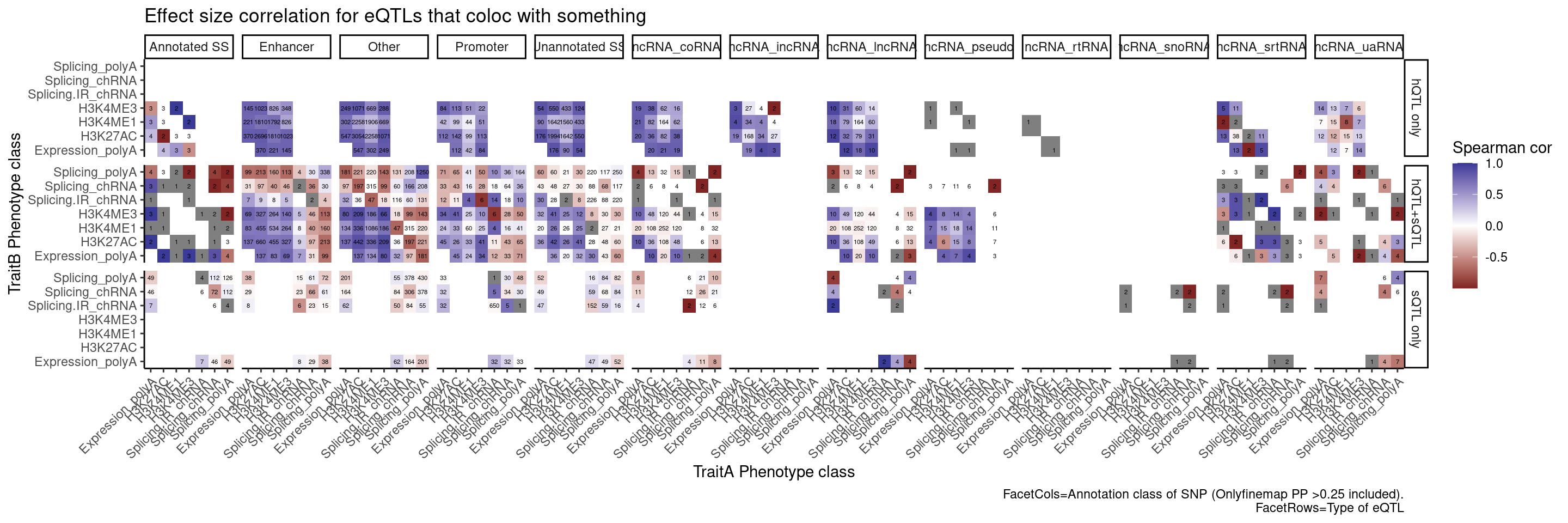
Perhaps we should plot the same ideas but breaking out the introns into classes by whether we have some good reason to think it would be an NMD target (ie unannoated, and or annotated with nonsense mediated decay transcript tag)
coloc.results.tidycolocalized %>%
  group_by(Locus, snp) %>%
  filter(any(PC=="Expression.Splicing.Subset_YRI")) %>%
  ungroup() %>%
  filter(PC %in% c("Expression.Splicing.Subset_YRI","H3K27AC", "H3K4ME1", "H3K4ME3", "polyA.Splicing.Subset_YRI", "chRNA.Splicing", "chRNA.IER")) %>%
  left_join(., ., by=c("Locus", "snp")) %>%
  filter(!((P.x == P.y) & (PC.x == PC.y))) %>%
  group_by(Locus, snp) %>%
  mutate(
    ContainsChromatinEqtl = any(PC.x %in% c("H3K27AC", "H3K4ME1", "H3K4ME3")),
    ContainsSqtl = any(PC.x %in% c("polyA.Splicing.Subset_YRI", "chRNA.Splicing", "chRNA.IER"))
    ) %>%
  ungroup() %>%
  mutate(Contains.eQTL_Contains.sQTL = paste(ContainsChromatinEqtl, ContainsSqtl)) %>%
  dplyr::select(-iteration.y) %>%
  left_join(
    finemap.snps.annotated %>%
      dplyr::select(SNP_iteration_locus, FinemapPP, AnnotationClass) %>%
      separate(SNP_iteration_locus, into=c("snp", "iteration.x", "Locus"), convert=T, sep="_")
  ) %>%
  filter(FinemapPP >0.25) %>%
  mutate(AnnotationSuperclass = case_when(
    str_detect(AnnotationClass, "Splice.+_1") ~ "Annotated SS",
    str_detect(AnnotationClass, "Splice.+_0$") ~ "Unannotated SS",
    str_detect(AnnotationClass, "Enhancer") ~ "Enhancer",
    str_detect(AnnotationClass, "Promoter") ~ "Promoter",
    TRUE ~ "Other"
  )) %>%
  mutate(PC.x = recode(PC.x, !!!PC.ShortAliases)) %>%
  mutate(PC.y = recode(PC.y, !!!PC.ShortAliases)) %>%
  mutate(Contains.eQTL_Contains.sQTL = recode(Contains.eQTL_Contains.sQTL,
                                              !!!c("TRUE TRUE"="hQTL+sQTL",
                                                   "TRUE FALSE"="hQTL only",
                                                   "FALSE TRUE"="sQTL only"))) %>%
  filter(Contains.eQTL_Contains.sQTL=="sQTL only" & AnnotationSuperclass=="Annotated SS") %>%
  ggplot(aes(x=beta.x, y=beta.y)) +
  geom_point() +
  geom_vline(xintercept=0) +
  geom_hline(yintercept=0) +
  facet_grid(rows=vars(PC.x), cols=vars(PC.y)) +
  theme_bw() +
  labs(x="TraitA Phenotype class", y="TraitB Phenotype class", title="Effect size correlation for eQTLs/sQTLs that are not hQTLs",
       caption = str_wrap("Only SNPs with finemap PP > 0.25 in annotated splice site SNP included"))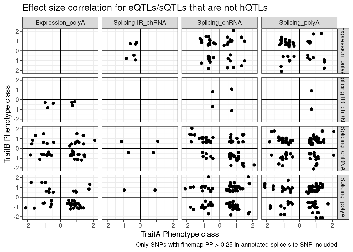
Write out bed files for meta QTL plot
As a side thing, I wrote a script to make metaQTL plots. That is, I lump the high/high allele genotypes for many QTLs and plot a metagene plot, along with the heterzygotes, and the low/low genotypes. This could be useful as an alternative to looking through a bunch of pygenometracks QTL plots. I think this list of eQTLs that coloc with hQTL only versus those that coloc with sQTL only would be a good test plot to look at. For example, I expect to see promoter effects at the hQTL eGenes but not so much at the sQTL eGenes, and definitely not at the sQTL eGenes with high finemapping probability as splice sites
sessionInfo()R version 3.6.1 (2019-07-05)
Platform: x86_64-pc-linux-gnu (64-bit)
Running under: CentOS Linux 7 (Core)
Matrix products: default
BLAS/LAPACK: /software/openblas-0.2.19-el7-x86_64/lib/libopenblas_haswellp-r0.2.19.so
locale:
[1] LC_CTYPE=en_US.UTF-8 LC_NUMERIC=C LC_TIME=C
[4] LC_COLLATE=C LC_MONETARY=C LC_MESSAGES=C
[7] LC_PAPER=C LC_NAME=C LC_ADDRESS=C
[10] LC_TELEPHONE=C LC_MEASUREMENT=C LC_IDENTIFICATION=C
attached base packages:
[1] stats graphics grDevices utils datasets methods base
other attached packages:
[1] qvalue_2.16.0 data.table_1.14.2 forcats_0.4.0 stringr_1.4.0
[5] dplyr_1.0.9 purrr_0.3.4 readr_1.3.1 tidyr_1.2.0
[9] tibble_3.1.7 ggplot2_3.3.6 tidyverse_1.3.0
loaded via a namespace (and not attached):
[1] httr_1.4.4 jsonlite_1.6 splines_3.6.1 R.utils_2.9.0
[5] modelr_0.1.8 assertthat_0.2.1 highr_0.9 cellranger_1.1.0
[9] yaml_2.2.0 pillar_1.7.0 backports_1.4.1 lattice_0.20-38
[13] glue_1.6.2 digest_0.6.20 promises_1.0.1 rvest_0.3.5
[17] colorspace_1.4-1 htmltools_0.5.3 httpuv_1.5.1 Matrix_1.2-18
[21] R.oo_1.22.0 plyr_1.8.4 pkgconfig_2.0.2 broom_1.0.0
[25] haven_2.3.1 scales_1.1.0 whisker_0.3-2 later_0.8.0
[29] git2r_0.26.1 mgcv_1.8-40 generics_0.1.3 farver_2.1.0
[33] ellipsis_0.3.2 withr_2.5.0 cli_3.3.0 magrittr_1.5
[37] crayon_1.3.4 readxl_1.3.1 evaluate_0.15 R.methodsS3_1.7.1
[41] fs_1.5.2 fansi_0.4.0 nlme_3.1-140 xml2_1.3.2
[45] tools_3.6.1 hms_0.5.3 lifecycle_1.0.1 munsell_0.5.0
[49] reprex_0.3.0 compiler_3.6.1 rlang_1.0.5 grid_3.6.1
[53] rstudioapi_0.14 labeling_0.3 rmarkdown_1.13 gtable_0.3.0
[57] DBI_1.1.0 reshape2_1.4.3 R6_2.4.0 lubridate_1.7.4
[61] knitr_1.39 fastmap_1.1.0 utf8_1.1.4 workflowr_1.6.2
[65] rprojroot_2.0.2 stringi_1.4.3 Rcpp_1.0.5 vctrs_0.4.1
[69] dbplyr_1.4.2 tidyselect_1.1.2 xfun_0.31