20220920_Explore_chRNA_sQTLs

Count number QTLs

…From permutation pass, with cis-eqtl test windows centered around the test phenotype.

library(tidyverse)
library(data.table)

Files <- Sys.glob("../code/QTLs/QTLTools/*/PermutationPass.FDR_Added.txt.gz")
Files

 [1] "../code/QTLs/QTLTools/CTCF/PermutationPass.FDR_Added.txt.gz"                               
 [2] "../code/QTLs/QTLTools/Expression.Splicing.Subset_YRI/PermutationPass.FDR_Added.txt.gz"     
 [3] "../code/QTLs/QTLTools/Expression.Splicing/PermutationPass.FDR_Added.txt.gz"                
 [4] "../code/QTLs/QTLTools/H3K27AC/PermutationPass.FDR_Added.txt.gz"                            
 [5] "../code/QTLs/QTLTools/H3K36ME3/PermutationPass.FDR_Added.txt.gz"                           
 [6] "../code/QTLs/QTLTools/H3K4ME1/PermutationPass.FDR_Added.txt.gz"                            
 [7] "../code/QTLs/QTLTools/H3K4ME3/PermutationPass.FDR_Added.txt.gz"                            
 [8] "../code/QTLs/QTLTools/MetabolicLabelled.30min.IER/PermutationPass.FDR_Added.txt.gz"        
 [9] "../code/QTLs/QTLTools/MetabolicLabelled.30min.IR/PermutationPass.FDR_Added.txt.gz"         
[10] "../code/QTLs/QTLTools/MetabolicLabelled.30min.IRjunctions/PermutationPass.FDR_Added.txt.gz"
[11] "../code/QTLs/QTLTools/MetabolicLabelled.30min.Splicing/PermutationPass.FDR_Added.txt.gz"   
[12] "../code/QTLs/QTLTools/MetabolicLabelled.30min/PermutationPass.FDR_Added.txt.gz"            
[13] "../code/QTLs/QTLTools/MetabolicLabelled.60min.IER/PermutationPass.FDR_Added.txt.gz"        
[14] "../code/QTLs/QTLTools/MetabolicLabelled.60min.IR/PermutationPass.FDR_Added.txt.gz"         
[15] "../code/QTLs/QTLTools/MetabolicLabelled.60min.IRjunctions/PermutationPass.FDR_Added.txt.gz"
[16] "../code/QTLs/QTLTools/MetabolicLabelled.60min.Splicing/PermutationPass.FDR_Added.txt.gz"   
[17] "../code/QTLs/QTLTools/MetabolicLabelled.60min/PermutationPass.FDR_Added.txt.gz"            
[18] "../code/QTLs/QTLTools/ProCap/PermutationPass.FDR_Added.txt.gz"                             
[19] "../code/QTLs/QTLTools/chRNA.Expression.Splicing/PermutationPass.FDR_Added.txt.gz"          
[20] "../code/QTLs/QTLTools/chRNA.Expression_cheRNA/PermutationPass.FDR_Added.txt.gz"            
[21] "../code/QTLs/QTLTools/chRNA.Expression_eRNA/PermutationPass.FDR_Added.txt.gz"              
[22] "../code/QTLs/QTLTools/chRNA.Expression_lncRNA/PermutationPass.FDR_Added.txt.gz"            
[23] "../code/QTLs/QTLTools/chRNA.Expression_ncRNA/PermutationPass.FDR_Added.txt.gz"             
[24] "../code/QTLs/QTLTools/chRNA.Expression_snoRNA/PermutationPass.FDR_Added.txt.gz"            
[25] "../code/QTLs/QTLTools/chRNA.IER/PermutationPass.FDR_Added.txt.gz"                          
[26] "../code/QTLs/QTLTools/chRNA.IR/PermutationPass.FDR_Added.txt.gz"                           
[27] "../code/QTLs/QTLTools/chRNA.IRjunctions/PermutationPass.FDR_Added.txt.gz"                  
[28] "../code/QTLs/QTLTools/chRNA.Slopes/PermutationPass.FDR_Added.txt.gz"                       
[29] "../code/QTLs/QTLTools/chRNA.Splicing.Order/PermutationPass.FDR_Added.txt.gz"               
[30] "../code/QTLs/QTLTools/chRNA.Splicing/PermutationPass.FDR_Added.txt.gz"                     
[31] "../code/QTLs/QTLTools/polyA.IER.Subset_YRI/PermutationPass.FDR_Added.txt.gz"               
[32] "../code/QTLs/QTLTools/polyA.IER/PermutationPass.FDR_Added.txt.gz"                          
[33] "../code/QTLs/QTLTools/polyA.IR.Subset_YRI/PermutationPass.FDR_Added.txt.gz"                
[34] "../code/QTLs/QTLTools/polyA.IR/PermutationPass.FDR_Added.txt.gz"                           
[35] "../code/QTLs/QTLTools/polyA.IRjunctions/PermutationPass.FDR_Added.txt.gz"                  
[36] "../code/QTLs/QTLTools/polyA.Splicing.Subset_YRI/PermutationPass.FDR_Added.txt.gz"          
[37] "../code/QTLs/QTLTools/polyA.Splicing/PermutationPass.FDR_Added.txt.gz"                     

Ok, actually, I think these files are out dated.

TODO: Make sure we have recently called these as snakemake target files, since Carlos updated these… I’m realizing there are lots and lots of things I just have to re-run from the snakemake before I can get up-to-date output files to do many QC types of analyses. So I’m going to to skip to only doing things with files that already exist as of today to get a sense of what results to expect once we finalize some analyses.

I think will mainly work with the colocalization output files here

Explore colocalization output

PhenotypeAliases <- read_tsv("../data/Phenotypes_recode_for_Plotting.txt")

PC.ShortAliases <- PhenotypeAliases %>%
  dplyr::select(PC, ShorterAlias) %>% deframe()

coloc.results <- read_tsv("../code/hyprcoloc/Results/ForColoc/MolColocStandard/results.txt.gz")

coloc.results.tidycolocalized <- read_tsv("../code/hyprcoloc/Results/ForColoc/MolColocStandard/tidy_results_OnlyColocalized.txt.gz") %>%
  separate(phenotype_full, into=c("PC", "P"), sep=";")

# Get all the phenotype classes
coloc.results.tidycolocalized$PC %>% unique()

 [1] "polyA.Splicing"                   "MetabolicLabelled.30min"         
 [3] "MetabolicLabelled.60min"          "H3K27AC"                         
 [5] "H3K4ME3"                          "H3K4ME1"                         
 [7] "chRNA.IER"                        "ProCap"                          
 [9] "polyA.Splicing.Subset_YRI"        "CTCF"                            
[11] "chRNA.Splicing.Order"             "chRNA.Expression_ncRNA"          
[13] "Expression.Splicing"              "Expression.Splicing.Subset_YRI"  
[15] "chRNA.Splicing"                   "MetabolicLabelled.30min.Splicing"
[17] "MetabolicLabelled.60min.Splicing" "chRNA.Expression.Splicing"       
[19] "H3K36ME3"                         "polyA.IER"                       
[21] "MetabolicLabelled.30min.IER"      "MetabolicLabelled.60min.IER"     
[23] "polyA.IER.Subset_YRI"             "chRNA.Slopes"                    

#How many YRI poly A QTLs
coloc.results.tidycolocalized %>%
  filter(PC=="Expression.Splicing.Subset_YRI")

# A tibble: 1,741 × 11
   snp      beta beta_se        p Locus PC    P     iteration ColocPr RegionalPr
   <chr>   <dbl>   <dbl>    <dbl> <chr> <chr> <chr>     <dbl>   <dbl>      <dbl>
 1 7:121…  0.561  0.119  9.18e- 6 ENSG… Expr… ENSG…         1   0.835      0.897
 2 7:199…  0.553  0.106  1.13e- 6 ENSG… Expr… ENSG…         1   0.308      0.531
 3 7:817…  1.69   0.143  8.35e-20 ENSG… Expr… ENSG…         1   0.896      0.923
 4 2:201…  0.388  0.0812 7.01e- 6 ENSG… Expr… ENSG…         1   0.940      0.963
 5 7:962… -0.335  0.0848 1.59e- 4 ENSG… Expr… ENSG…         3   0.634      0.697
 6 17:72…  0.324  0.0620 1.15e- 6 ENSG… Expr… ENSG…         1   0.959      0.986
 7 7:268…  0.554  0.110  2.71e- 6 ENSG… Expr… ENSG…         2   0.975      0.977
 8 6:822… -0.185  0.0337 4.12e- 7 ENSG… Expr… ENSG…         1   0.621      0.787
 9 11:33…  0.281  0.0475 6.45e- 8 ENSG… Expr… ENSG…         2   0.276      0.528
10 17:35… -0.526  0.108  4.95e- 6 ENSG… Expr… ENSG…         3   0.905      0.954
# … with 1,731 more rows, and 1 more variable: TopSNPFinemapPr <dbl>

#Of which, how many also contain chromatin
coloc.results.tidycolocalized %>%
  filter(PC=="Expression.Splicing.Subset_YRI")

# A tibble: 1,741 × 11
   snp      beta beta_se        p Locus PC    P     iteration ColocPr RegionalPr
   <chr>   <dbl>   <dbl>    <dbl> <chr> <chr> <chr>     <dbl>   <dbl>      <dbl>
 1 7:121…  0.561  0.119  9.18e- 6 ENSG… Expr… ENSG…         1   0.835      0.897
 2 7:199…  0.553  0.106  1.13e- 6 ENSG… Expr… ENSG…         1   0.308      0.531
 3 7:817…  1.69   0.143  8.35e-20 ENSG… Expr… ENSG…         1   0.896      0.923
 4 2:201…  0.388  0.0812 7.01e- 6 ENSG… Expr… ENSG…         1   0.940      0.963
 5 7:962… -0.335  0.0848 1.59e- 4 ENSG… Expr… ENSG…         3   0.634      0.697
 6 17:72…  0.324  0.0620 1.15e- 6 ENSG… Expr… ENSG…         1   0.959      0.986
 7 7:268…  0.554  0.110  2.71e- 6 ENSG… Expr… ENSG…         2   0.975      0.977
 8 6:822… -0.185  0.0337 4.12e- 7 ENSG… Expr… ENSG…         1   0.621      0.787
 9 11:33…  0.281  0.0475 6.45e- 8 ENSG… Expr… ENSG…         2   0.276      0.528
10 17:35… -0.526  0.108  4.95e- 6 ENSG… Expr… ENSG…         3   0.905      0.954
# … with 1,731 more rows, and 1 more variable: TopSNPFinemapPr <dbl>

coloc.results.tidycolocalized %>%
  group_by(Locus, snp) %>%
  filter(any(PC=="Expression.Splicing.Subset_YRI")) %>%
  summarise(
    ContainsChromatinEqtl = any(PC %in% c("H3K27AC", "H3K4ME1", "H3K4ME3")),
    ContainsSqtl = any(PC %in% c("polyA.Splicing.Subset_YRI", "chRNA.Splicing", "chRNA.IER"))
    ) %>%
  ggplot(aes(x=1, fill=paste(ContainsChromatinEqtl, ContainsSqtl))) +
  geom_bar() +
  labs(title="More chromatin localization with eQTLs than splicing", y="Number of colocalizing eQTLs") +
  theme_classic() +
  theme(axis.title.x=element_blank(),
        axis.text.x=element_blank(),
        axis.ticks.x=element_blank())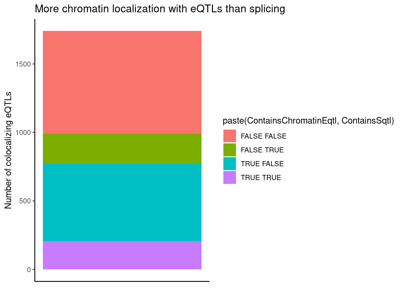

Is this plot sensitive to whether I call just consider H3K27AC for chromatin, as opposed to H3K4ME3

bind_rows(
  coloc.results.tidycolocalized %>%
    group_by(Locus, snp) %>%
    filter(any(PC=="Expression.Splicing.Subset_YRI")) %>%
    summarise(
      ContainsChromatinEqtl = any(PC %in% c("H3K27AC", "H3K4ME3", "H3K4ME1")),
      ContainsSqtl = any(PC %in% c("polyA.Splicing.Subset_YRI", "chRNA.Splicing", "chRNA.IER"))
      ) %>%
    mutate(x="chromatin = H3K4ME3|H3K4ME1|H3K27AC; splicing=chRNA|polyA"),
  coloc.results.tidycolocalized %>%
    group_by(Locus, snp) %>%
    filter(any(PC=="Expression.Splicing.Subset_YRI")) %>%
    summarise(
      ContainsChromatinEqtl = any(PC %in% c("H3K27AC")),
      ContainsSqtl = any(PC %in% c("polyA.Splicing.Subset_YRI", "chRNA.Splicing", "chRNA.IER"))
      ) %>%
    mutate(x="chromatin = H3K27AC; splicing=chRNA|polyA"),
  coloc.results.tidycolocalized %>%
    group_by(Locus, snp) %>%
    filter(any(PC=="Expression.Splicing.Subset_YRI")) %>%
    summarise(
      ContainsChromatinEqtl = any(PC %in% c("H3K4ME3")),
      ContainsSqtl = any(PC %in% c("polyA.Splicing.Subset_YRI", "chRNA.Splicing", "chRNA.IER"))
      ) %>%
    mutate(x="chromatin = H3K4ME3; splicing=chRNA|polyA no IR"),
  coloc.results.tidycolocalized %>%
    group_by(Locus, snp) %>%
    filter(any(PC=="Expression.Splicing.Subset_YRI")) %>%
    summarise(
      ContainsChromatinEqtl = any(PC %in% c("H3K27AC", "H3K4ME3", "H3K4ME1")),
      ContainsSqtl = any(PC %in% c("polyA.Splicing.Subset_YRI", "chRNA.Splicing"))
      ) %>%
    mutate(x="chromatin = H3K27AC; splicing=chRNA|polyA no IR"),
  coloc.results.tidycolocalized %>%
    group_by(Locus, snp) %>%
    filter(any(PC=="Expression.Splicing.Subset_YRI")) %>%
    summarise(
      ContainsChromatinEqtl = any(PC %in% c("H3K27AC", "H3K4ME3", "H3K4ME1")),
      ContainsSqtl = any(PC %in% c("polyA.Splicing.Subset_YRI"))
      ) %>%
    mutate(x="chromatin = H3K27AC; splicing=polyA"),
  coloc.results.tidycolocalized %>%
    group_by(Locus, snp) %>%
    filter(any(PC=="Expression.Splicing.Subset_YRI")) %>%
    summarise(
      ContainsChromatinEqtl = any(PC %in% c("H3K27AC", "H3K4ME3", "H3K4ME1")),
      ContainsSqtl = any(PC %in% c("chRNA.Splicing", "chRNA.IER"))
      ) %>%
    mutate(x="chromatin = H3K27AC; splicing=chRNA"),
  coloc.results.tidycolocalized %>%
    group_by(Locus, snp) %>%
    filter(any(PC=="Expression.Splicing.Subset_YRI")) %>%
    summarise(
      ContainsChromatinEqtl = any(PC %in% c("H3K27AC", "H3K4ME3", "H3K4ME1")),
      ContainsSqtl = any(PC %in% c("chRNA.Splicing"))
      ) %>%
    mutate(x="chromatin = H3K27AC; splicing=chRNA no IR")
  ) %>%
  ggplot(aes(x=x, fill=paste(ContainsChromatinEqtl, ContainsSqtl))) +
  geom_bar() +
  labs(title="More chromatin localization with eQTLs than splicing", y="Number of colocalizing eQTLs", x="") +
  theme_classic() +
  theme(axis.text.x = element_text(angle = 45, vjust = 1, hjust=1))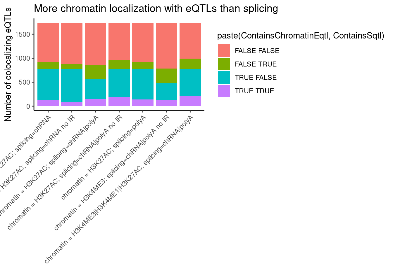

I am curious about these QTLs that colocalize both chromatinQTL and sQTL effects. I will have to look at enrichment of SNP annotations under finemapping results (which I will look at later in this notebook I think) to get some sense of if they are mostly driven by splicing effects or by chromatin effects.

Next, let’s look at the direction of effects in each of these categories. For example, I expect (and have shown previously) that direction of chromatin QTL effects and eQTL effects are very concordant in colocalizing QTLs (eg Spearman correlation coef >0.9). Are intron retention effects generally discordant in these genes with an intron retention QTL colocalizing with eQTL? Biologically I expect intron retention to generally down regulate. But then I suspect some intron retention QTL effects are somehow picking up on positive transcription effects. So I’m not exactly sure what to expect…

coloc.results.tidycolocalized %>%
  group_by(Locus, snp) %>%
  filter(any(PC=="Expression.Splicing.Subset_YRI")) %>%
  ungroup() %>%
  filter(PC %in% c("Expression.Splicing.Subset_YRI","H3K27AC", "H3K4ME1", "H3K4ME3", "polyA.Splicing.Subset_YRI", "chRNA.Splicing", "chRNA.IER")) %>%
  left_join(., ., by=c("Locus", "snp")) %>%
  filter(!((P.x == P.y) & (PC.x == PC.y))) %>% 
  group_by(Locus, snp) %>%
  mutate(
    ContainsChromatinEqtl = any(PC.x %in% c("H3K27AC", "H3K4ME1", "H3K4ME3")),
    ContainsSqtl = any(PC.x %in% c("polyA.Splicing.Subset_YRI", "chRNA.Splicing", "chRNA.IER"))
    ) %>%
  ungroup() %>%
  mutate(Contains.eQTL_Contains.sQTL = paste(ContainsChromatinEqtl, ContainsSqtl)) %>%
  group_by(Contains.eQTL_Contains.sQTL, PC.x, PC.y) %>%
  summarise(cor = cor(beta.x, beta.y, method="spearman")) %>%
  mutate(PC.x = recode(PC.x, !!!PC.ShortAliases)) %>%
  mutate(PC.y = recode(PC.y, !!!PC.ShortAliases)) %>%
  ggplot(aes(x=PC.x, y=PC.y, fill=cor)) +
  geom_raster() +
  scale_fill_gradient2() +
  facet_wrap(~Contains.eQTL_Contains.sQTL) +
  scale_x_discrete(expand=c(0,0)) +
  scale_y_discrete(expand=c(0,0)) +
  theme_classic() +
  theme(axis.text.x = element_text(angle = 45, vjust = 1, hjust=1)) +
  labs(x="TraitA Phenotype class", y="TraitB Phenotype class", fill="Spearman cor", title="Effect size correlation",
       caption = "FacetTitle: IsChromatinQTL IsSplicingQTL")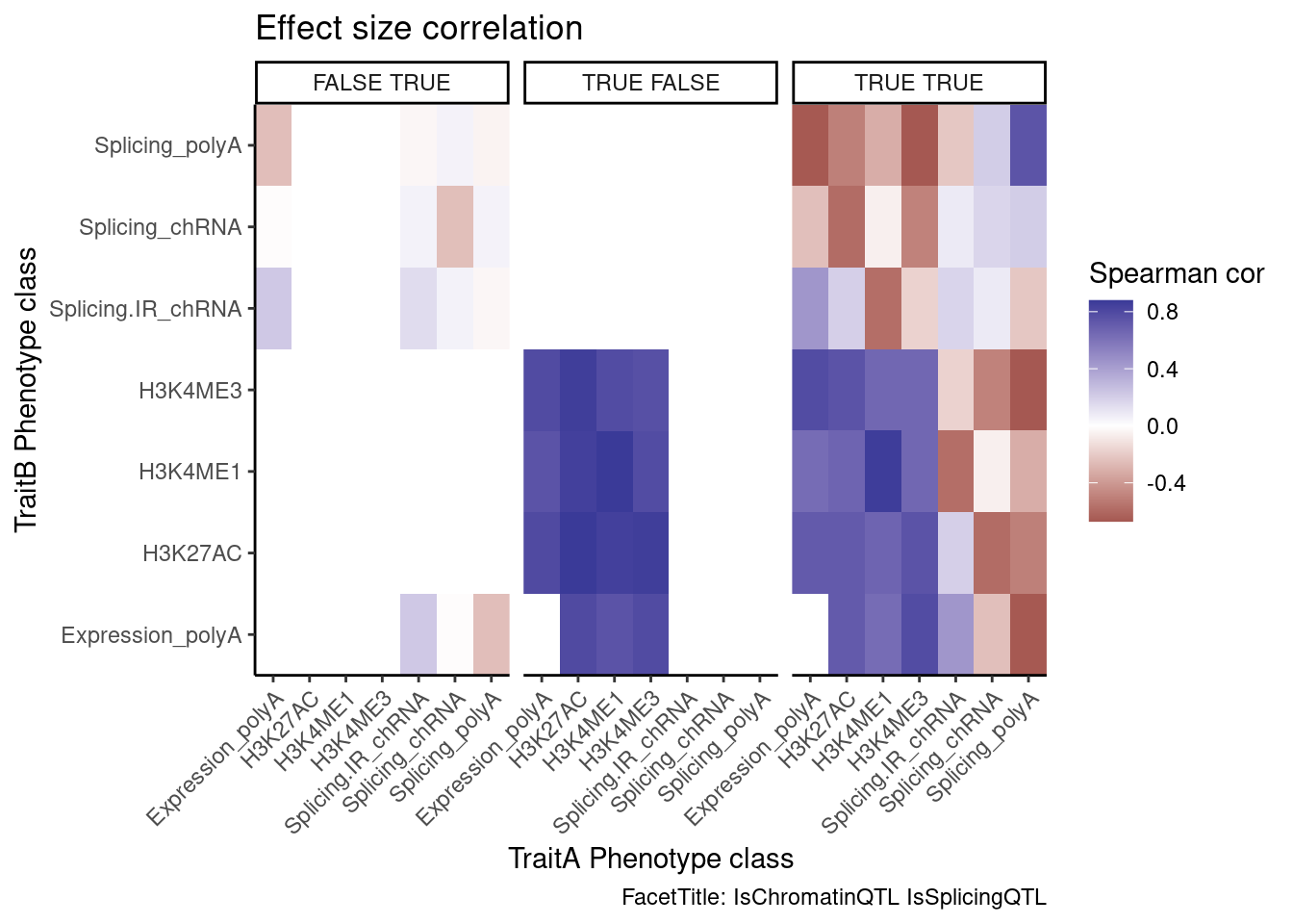

Hmm, it seems that intron retention might just be picking up eQTL signals, since it is positively correlated with eQTL effect size. And I don’t know how to explain that sQTLs are generally anti-correlated with eQTL effects in polyA (I would’ve expected no correlation).

And thankfully at least the effect directions of the chRNA sQTLs are positively correlated with the polyA sQTLs. These are all to be expected.

Next I want to plot a lot of these examples, as sashimi plots and coverage plots grouped by genotype of the top SNP, to get some intuitions on this. More specifically, is PSI larger in chRNA for the effects of opposite direction sQTL/eQTL effects (the presumed NMD targets)?

# AllFeats <- read_tsv("../code/QC/AllQTLPhenotypes.PermutationTest.bed.gz", col_names=c("Chrom", "start", "stop", "name", "score", "strand", "thickStart","thickStop", "Color")) %>%
#   separate(name, into=c("PC", "P", "topSNP.QTLTools", "Pval", "FDR"), convert=T, sep=";")

AllFeats <- Sys.glob("../code/QTLs/QTLTools/*/OnlyFirstReps.sorted.qqnorm.bed.gz") %>%
  setNames(str_replace(., "../code/QTLs/QTLTools/(.+?)/OnlyFirstReps.sorted.qqnorm.bed.gz", "\\1")) %>%
  lapply(fread, sep='\t', select=1:6) %>%
  bind_rows(.id="PC")

sample_n_of <- function(data, size, ...) {
  dots <- quos(...)
  
  group_ids <- data %>% 
    group_by(!!! dots) %>% 
    group_indices()
  
  sampled_groups <- sample(unique(group_ids), size)
  
  data %>% 
    filter(group_ids %in% sampled_groups)
}

ColocsToPlot.dat <- coloc.results.tidycolocalized %>%
  filter(PC %in% c("Expression.Splicing.Subset_YRI","H3K27AC", "H3K4ME1", "H3K4ME3", "polyA.Splicing.Subset_YRI", "chRNA.Splicing", "chRNA.IER")) %>%
  group_by(Locus, snp) %>%
  filter(any(PC=="Expression.Splicing.Subset_YRI")) %>%
  mutate(
    ContainsChromatinEqtl = if_else(any(PC %in% c("H3K27AC", "H3K4ME1", "H3K4ME3")), "hQTL", "Not_hQTL"),
    ContainsSqtl = if_else(any(PC %in% c("polyA.Splicing.Subset_YRI", "chRNA.Splicing", "chRNA.IER")), "sQTL", "Not_sQTL")
    ) %>%
  ungroup() %>%
  mutate(Group = paste(ContainsChromatinEqtl, ContainsSqtl, sep=".")) %>%
  inner_join(AllFeats, by=c("PC", "P"="pid"))

set.seed(0)
ColocsToPlot.Subset <- ColocsToPlot.dat %>%
  distinct(Locus, snp, Group, iteration) %>%
  group_by(Group) %>%
  sample_n(100) %>%
  ungroup()

Write bash script and other necessary stuff to execute my helper script for plotting

#Create folder to house files and images
dir.create("../code/scratch/20220921_PlotColocs")

# Write bed files containing all colocalized features that will be plotted
ColocsToPlot.dat %>%
  inner_join(ColocsToPlot.Subset) %>%
  mutate(PC = recode(PC, !!!PC.ShortAliases)) %>%
  mutate(name=paste(PC, P, "beta=",signif(beta, 2)),
         dummyScore = 0) %>%
  dplyr::select(`#Chr`, start, end, name, dummyScore, strand) %>%
  write_tsv("../code/scratch/20220921_PlotColocs/.ColocFeats.bed")

# Write pygenometracks ini file for the above bed file
fileConn<-file("../code/scratch/20220921_PlotColocs/.ColocFeats.ini")
writeLines(c("[feats]",
             "type = bed",
             "file = scratch/20220921_PlotColocs/.ColocFeats.bed",
             "fontsize = 3",
             "gene_rows = 10",
             "height=5"
             ), con=fileConn)
close(fileConn)

# Write a "groups" file for my custom script to determine which tracks to plot, and how to plot them
read_tsv("../code/scratch/bwList.Groups2.tsv") %>%
  filter(Group_label %in% c("chRNA", "polyA.RNA", "MetabolicLabelled.30min", "MetabolicLabelled.60min","H3K27AC", "H3K4ME3", "H3K4ME1", "H3K36ME3")) %>%
  write_tsv("../code/scratch/20220921_PlotColocs/.groups.tsv")

# Write a bash script that calls my custom script and pygenometracks to plot stuff
ColocsToPlot.dat %>%
  inner_join(ColocsToPlot.Subset) %>%
  rename(chrom="#Chr") %>%
  group_by(Locus, snp, chrom, Group, iteration) %>%
  summarise(
    min = min(start)-10,
    max= max(end)+10) %>%
  ungroup() %>%
  mutate(SnpPos = str_replace(snp, "^(.+?):(.+?):.+?:.+?$", "chr\\1:\\2")) %>%
  mutate(chrom.num = str_replace(chrom, "chr(.+?)$", "\\1")) %>%
  mutate(cmd = str_glue("python scripts/GenometracksByGenotype/AggregateBigwigsForPlotting.py --GroupSettingsFile scratch/20220921_PlotColocs/.groups.tsv --BigwigList scratch/bwList.tsv --SnpPos {SnpPos} --Normalization WholeGenome --Region {chrom}:{min}-{max} --BigwigListType KeyFile --OutputPrefix scratch/20220921_PlotColocs/. --VCF Genotypes/1KG_GRCh38/{chrom.num}.vcf.gz -vv --TracksTemplate scripts/GenometracksByGenotype/tracks_templates/GeneralPurposeColoredByGenotype.ini --Bed12GenesToIni scripts/GenometracksByGenotype/PremadeTracks/gencode.v26.FromGTEx.genes.bed12.gz  --FilterJuncsByBed scratch/20220921_PlotColocs/.ColocFeats.bed\npyGenomeTracks --tracks <(cat scratch/20220921_PlotColocs/.tracks.ini scratch/20220921_PlotColocs/.ColocFeats.ini) --out scratch/20220921_PlotColocs/{Group}.{Locus}.{iteration}.pdf --region {chrom}:{min}-{max} --title {Group}_{Locus}_{snp} --trackLabelFraction 0.15\n\n")) %>%
  dplyr::select(cmd) %>%
  write.table("../code/scratch/20220921_PlotColocs/MakePlots.sh", quote=F, row.names = F, col.names = F)

and execute the bash script to make a bunch of plots

cd /project2/yangili1/bjf79/ChromatinSplicingQTLs/code
bash scratch/20220921_PlotColocs/MakePlots.sh

I’ve browsed perhaps 50 so far… some things i’ve noticed:

• a lot of plots aren’t interpretable… or the eQTL effects are barely noticeable in this raw coverage plot at the given scale
• among the eQTL + sQTL + hQTL ones, a fair number of the interpretable ones are alt TSS
• among the sQTL + eQTL ones, often we see intron retention things (not in always understandable ways yet) around the sQTLs
• some NMD targets, though it’s not always more apparent in chRNA like I hypothesize
• TODO:May want to get a better sense of the chRNA-specific sQTLs
• TODO:Add annotations to plot about which introns are annotated or known NMD-related introns

Next, let’s compare these groups of eQTLs (those that coloc with sQTL only, with hQTL only, or with both), to “unexplained eQTLs” (in this case, ones that colocalize with something, but not sQTL or hQTL), in terms of their finemap SNP enrichment over annotations (eg ChromHMM states, splice sites, etc)…

dat <- fread("../code/QTL_SNP_Enrichment/FinemapIntersections/MolColocStandard.bed.gz", col.names=c("SNP_chrom", "SNP_start", "SNP_end", "SNP", "PosteriorPr", "Annotation_chrom", "Annotation_start", "Annotation_stop", "Annotation", "Overlap")) %>%
  separate(SNP, into=c("SNP", "HyprcolocCluster", "GeneLocus"), sep="_")


GeneLocus_Cluster_QTLSets <- ColocsToPlot.dat %>%
  distinct(Locus, iteration, Group) %>%
  unite(Locus.iteration, Locus, iteration) %>%
  rename(ClusterGroup=Group) %>%
  split(.$ClusterGroup)
  

#Define the function
PlotDifferentialEnrichmentBetweenQTLSets <- function(dat, GeneLocus_Cluster_QTLSet1, GeneLocus_Cluster_QTLSet2, seed=0, iterations=100){
  #GeneLocus_Cluster_QTLSet1 and GeneLocus_Cluster_QTLSet2 are dataframes with mandatory columns called Locus.iteration (with values of Locus_iteration), and a ClusterGroup column to name the two sets (ie value like "SplicingClusters" for GeneLocus_Cluster_QTLSet1 and "HistoneClusters" for GeneLocus_Cluster_QTLSet2)
  output <- list()
  results <- list()
  for (i in 1:iterations){
    results[[i]] <-
    bind_rows(
    sample_frac(GeneLocus_Cluster_QTLSet1, replace=T),
    sample_frac(GeneLocus_Cluster_QTLSet2, replace=T),
    .id="QTL.Set") %>%
    left_join(
      dat %>%
      mutate(Locus.iteration = paste(GeneLocus, HyprcolocCluster, sep="_")),
      by = "Locus.iteration"
    ) %>%
    mutate(Annotation = str_replace_all(Annotation, "_0$", "_UnannotatedButObserved")) %>%
    mutate(Annotation = str_replace_all(Annotation, "_1$", "_Annotated")) %>%
    mutate(Annotation = str_replace_all(Annotation, "^\\d+?_", "ChromHMM:")) %>%
    filter(!is.na(Annotation)) %>%
    mutate(Annotation = if_else(Annotation==".", "No annotation", Annotation)) %>%
    group_by(Annotation, ClusterGroup, QTL.Set) %>%
    summarise(Sum = sum(PosteriorPr)) %>%
    group_by(ClusterGroup, QTL.Set) %>%
    mutate(FractionAnnotatedPosteriorInGroup = Sum/sum(Sum, na.rm=T)) %>%
    ungroup() %>%
    # select(-ClusterGroup) %>%
    pivot_wider(names_from = "QTL.Set", values_from = c("FractionAnnotatedPosteriorInGroup", "Sum"), id_cols="Annotation") %>%
    mutate(Enrichment = FractionAnnotatedPosteriorInGroup_1/FractionAnnotatedPosteriorInGroup_2) %>%
    mutate(i=i)
  }
  output[["data"]] <- bind_rows(results)
  output[["plot"]] <- output[["data"]] %>%
  group_by(Annotation) %>%
  summarise(mean = exp(mean(log(Enrichment), na.rm=T)),
            Percentile10 = quantile(Enrichment, probs = 0.05, na.rm=T),
            Percentile90 = quantile(Enrichment, probs = 0.95, na.rm=T)) %>%
  ggplot(aes(x=Annotation, y=log2(mean))) +
    geom_hline(yintercept = 0, color='red') +
    geom_col() +
    geom_errorbar(aes(ymin=log2(Percentile10), ymax=log2(Percentile90))) +
    theme_bw() +
    # scale_y_continuous(trans='log2') +
    theme(axis.text.x = element_text(angle = 45, vjust = 1, hjust=1)) +
    coord_flip() +
    labs(x = "Annotation", y="Finemapping posterior mass relative log2 fold enrichment\nQTL.Set2 <----> QTL.Set1",
         caption = "Bootsrapped 90% confidence interval")
  return(output)
}

Ok now that I have the plotting function set up, let’s compare the eQTLs with hQTL but not sQTL, to those without sQTL or hQTL…

PlotDifferentialEnrichmentBetweenQTLSets(dat, GeneLocus_Cluster_QTLSets[["hQTL.Not_sQTL"]], GeneLocus_Cluster_QTLSets[["Not_hQTL.Not_sQTL"]])$plot +
  labs(caption="Set1=hQTL.Not_sQTL\nSet2=Not_hQTL.Not_sQTL")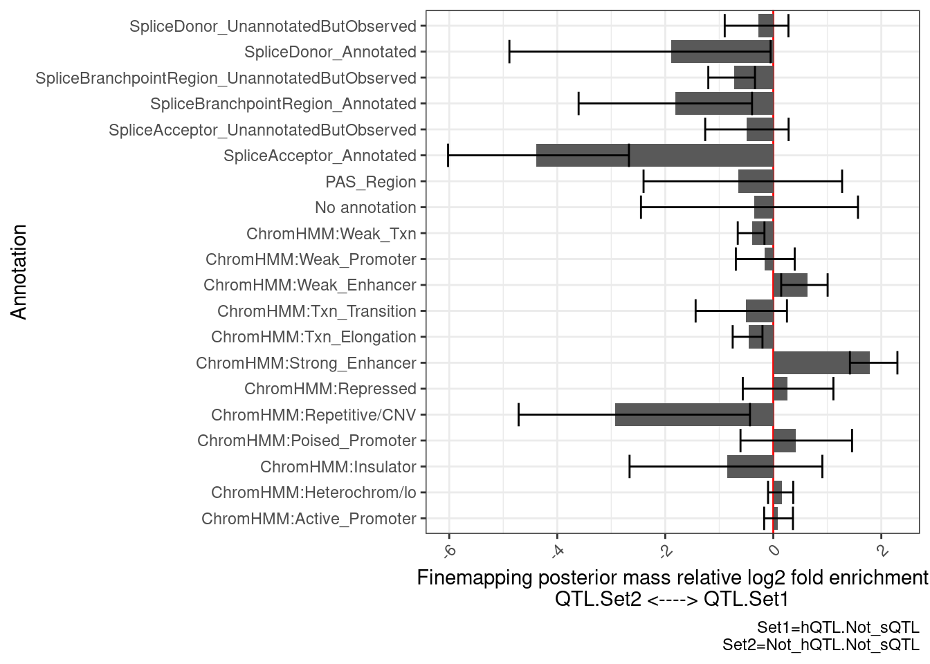

there is enrichment in ChromHMM enhancer regions, and de-enrichment in splice sites, as expected.

…And now check those eQTLs with sQTLs but not hQTLs, to those without hQTLs or sQTLs

PlotDifferentialEnrichmentBetweenQTLSets(dat, GeneLocus_Cluster_QTLSets[["Not_hQTL.sQTL"]], GeneLocus_Cluster_QTLSets[["Not_hQTL.Not_sQTL"]])$plot +
  labs(caption="Set1=Not_hQTL.sQTL\nSet2=Not_hQTL.Not_sQTL")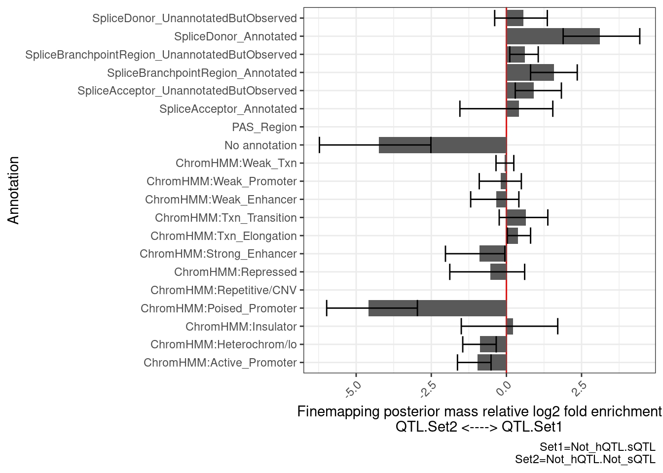

…Enrichment for splice sites as expected… Now let’s check those with both hQTLs or sQTLs to those without either…

PlotDifferentialEnrichmentBetweenQTLSets(dat, GeneLocus_Cluster_QTLSets[["hQTL.sQTL"]], GeneLocus_Cluster_QTLSets[["Not_hQTL.Not_sQTL"]])$plot +
  labs(caption="Set1=hQTL.sQTL\nSet2=Not_hQTL.Not_sQTL")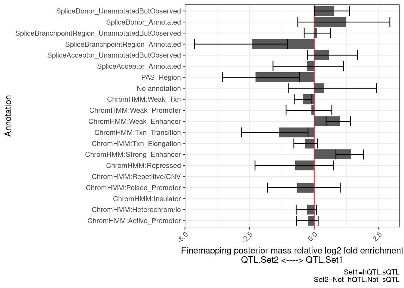

…so there is enrichment for PAS, that makes sense at it is a non splicing and non histone mechanism that can to regulate expression.

ncRNA QTLs

I think i want to also plot a lot of the new ncRNA QTLs… Let’s explore those

i would like to explore some of the following ideas:

• upstream antisense ncRNAs (from bidirectional promoter for a gene), which i expect to always have concordant effects with the gene.
• check for intergenic ncRNAs. I expect them to largely be concordant too, as they may be products of active enhancers that also affect a gene. However i will be curious to check for cases where the signs are non concordant, to make sure I even believe them…

ncRNA.annotations <- read_tsv("../code/NonCodingRNA_annotation/annotation/ncRNA.annotation.tab.gz")

head(ncRNA.annotations)

# A tibble: 6 × 9
  gene_name rna_type uaRNA coRNA            rtRNA ctRNA lncRNA snoRNA pseudogene
  <chr>     <chr>    <chr> <chr>            <chr> <chr> <chr>  <chr>  <chr>     
1 ncRNA_1   incRNA   .     .                .     .     .      .      .         
2 ncRNA_2   incRNA   .     .                .     .     .      .      .         
3 ncRNA_3   srtRNA   .     .                ENSG… .     .      .      .         
4 ncRNA_4   srtRNA   .     .                ENSG… .     .      .      .         
5 ncRNA_5   coRNA    .     ENSG00000217801… .     .     .      .      .         
6 ncRNA_8   rtRNA    .     .                ncRN… .     .      .      .         

ncRNA.annotations %>%
  count(rna_type) %>%
  arrange(desc(n))

# A tibble: 45 × 2
   rna_type         n
   <chr>        <int>
 1 srtRNA        5023
 2 incRNA        4924
 3 uaRNA         1609
 4 coRNA          362
 5 uaRNA,coRNA    303
 6 uaRNA,srtRNA   230
 7 rtRNA          164
 8 coRNA,srtRNA    90
 9 coRNA,pseudo    78
10 ctRNA           71
# … with 35 more rows

coloc.results.tidycolocalized %>%
  filter(PC == "chRNA.Expression_ncRNA")

# A tibble: 1,760 × 11
   snp      beta beta_se        p Locus PC    P     iteration ColocPr RegionalPr
   <chr>   <dbl>   <dbl>    <dbl> <chr> <chr> <chr>     <dbl>   <dbl>      <dbl>
 1 11:64… -0.420  0.0572 1.26e-10 ENSG… chRN… ncRN…         2   0.992      0.993
 2 17:48… -0.310  0.0816 2.69e- 4 ENSG… chRN… ncRN…         1   0.675      0.790
 3 2:372… -0.611  0.122  2.90e- 6 ENSG… chRN… ncRN…         1   0.850      0.880
 4 1:331…  1.02   0.193  8.69e- 7 ENSG… chRN… ncRN…         2   0.818      0.832
 5 17:47… -0.460  0.0894 1.72e- 6 ENSG… chRN… ENSG…         1   0.972      0.996
 6 7:873… -0.961  0.119  4.28e-12 ENSG… chRN… ENSG…         2   0.862      0.884
 7 7:873… -0.961  0.119  4.28e-12 ENSG… chRN… ENSG…         2   0.852      0.880
 8 6:822… -0.385  0.102  3.15e- 4 ENSG… chRN… ENSG…         1   0.621      0.787
 9 17:45… -1.03   0.147  5.36e-10 ENSG… chRN… ENSG…         2   0.962      0.968
10 17:35…  0.490  0.0999 4.39e- 6 ENSG… chRN… ENSG…         1   0.846      0.973
# … with 1,750 more rows, and 1 more variable: TopSNPFinemapPr <dbl>

Hmmm, this is kind of complicated but for simplicity for now, let’s just consider the ncRNAs with only one type of rna_type subannotation.

First, let’s confirm that effect sizes are generally concordant with eQTL and enhancer/promoter activity…

coloc.results.tidycolocalized$PC %>% unique()

 [1] "polyA.Splicing"                   "MetabolicLabelled.30min"         
 [3] "MetabolicLabelled.60min"          "H3K27AC"                         
 [5] "H3K4ME3"                          "H3K4ME1"                         
 [7] "chRNA.IER"                        "ProCap"                          
 [9] "polyA.Splicing.Subset_YRI"        "CTCF"                            
[11] "chRNA.Splicing.Order"             "chRNA.Expression_ncRNA"          
[13] "Expression.Splicing"              "Expression.Splicing.Subset_YRI"  
[15] "chRNA.Splicing"                   "MetabolicLabelled.30min.Splicing"
[17] "MetabolicLabelled.60min.Splicing" "chRNA.Expression.Splicing"       
[19] "H3K36ME3"                         "polyA.IER"                       
[21] "MetabolicLabelled.30min.IER"      "MetabolicLabelled.60min.IER"     
[23] "polyA.IER.Subset_YRI"             "chRNA.Slopes"                    

coloc.results.tidycolocalized %>%
  group_by(Locus, snp) %>%
  filter(any(PC=="Expression.Splicing.Subset_YRI") & any(PC=="chRNA.Expression_ncRNA")) %>%
  ungroup() %>%
  filter(PC %in% c("Expression.Splicing.Subset_YRI","H3K27AC", "H3K4ME1", "H3K4ME3", "chRNA.Expression_ncRNA")) %>%
  left_join(., ., by=c("Locus", "snp")) %>%
  filter(!((P.x == P.y) & (PC.x == PC.y))) %>%
  group_by(PC.x, PC.y) %>%
  summarise(cor = cor(beta.x, beta.y, method="spearman")) %>%
  mutate(PC.x = recode(PC.x, !!!PC.ShortAliases)) %>%
  mutate(PC.y = recode(PC.y, !!!PC.ShortAliases)) %>%
  ggplot(aes(x=PC.x, y=PC.y, fill=cor)) +
  geom_raster() +
  scale_fill_gradient2() +
  scale_x_discrete(expand=c(0,0)) +
  scale_y_discrete(expand=c(0,0)) +
  theme_classic() +
  theme(axis.text.x = element_text(angle = 45, vjust = 1, hjust=1)) +
  labs(x="TraitA Phenotype class", y="TraitB Phenotype class", fill="Spearman cor", title="Effect size correlation")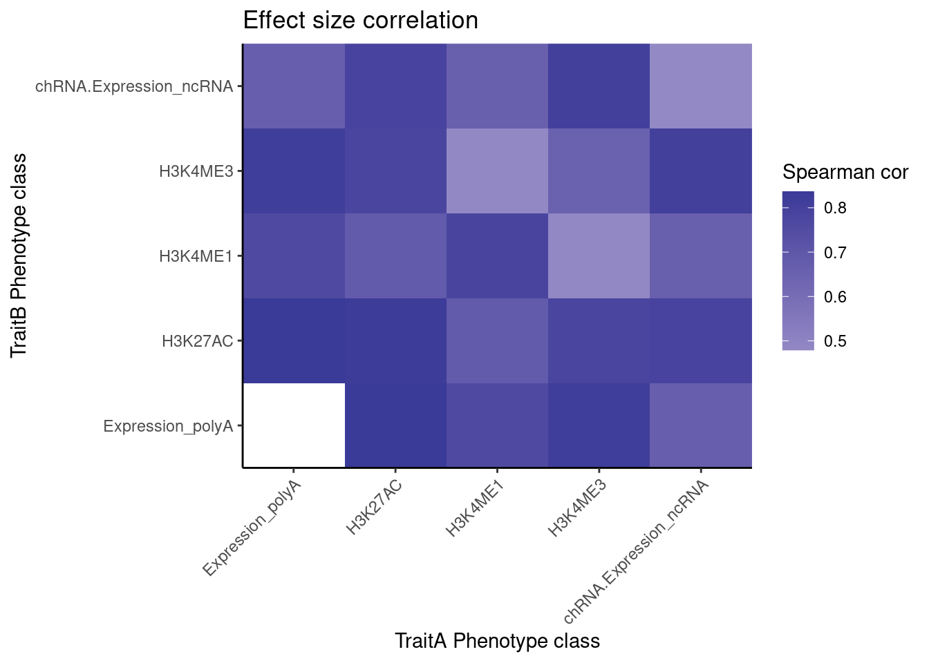

Ok, now let’s break up the ncRNA phenotypes into the sub-groups…

This is a simplified way of doing this because the ncRNA annotation file is a bit complicated and i don’t fully know how to handle it yet.

ncRNA.annotations %>%
  count(rna_type) %>%
  ggplot(aes(x=rna_type, y=n)) +
  coord_flip() +
  geom_col()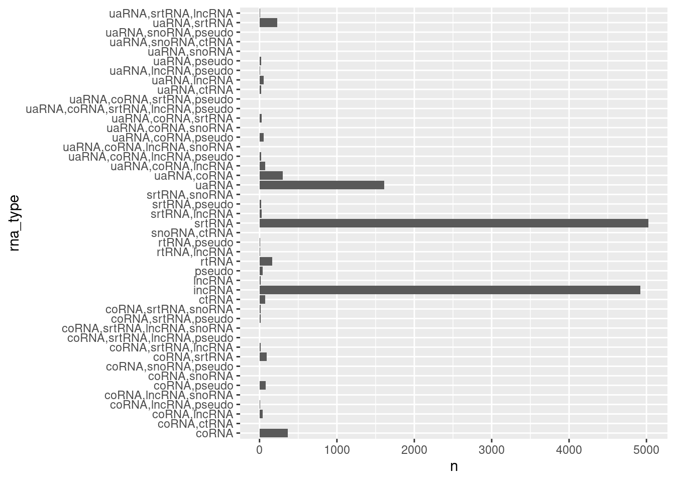

#For simplicity, Only consider ncRNAs that only have one subtype
ncRNA.annotations %>%
  filter(!str_detect(rna_type, ",") )%>%
  count(rna_type) %>%
  ggplot(aes(x=rna_type, y=n)) +
  geom_col()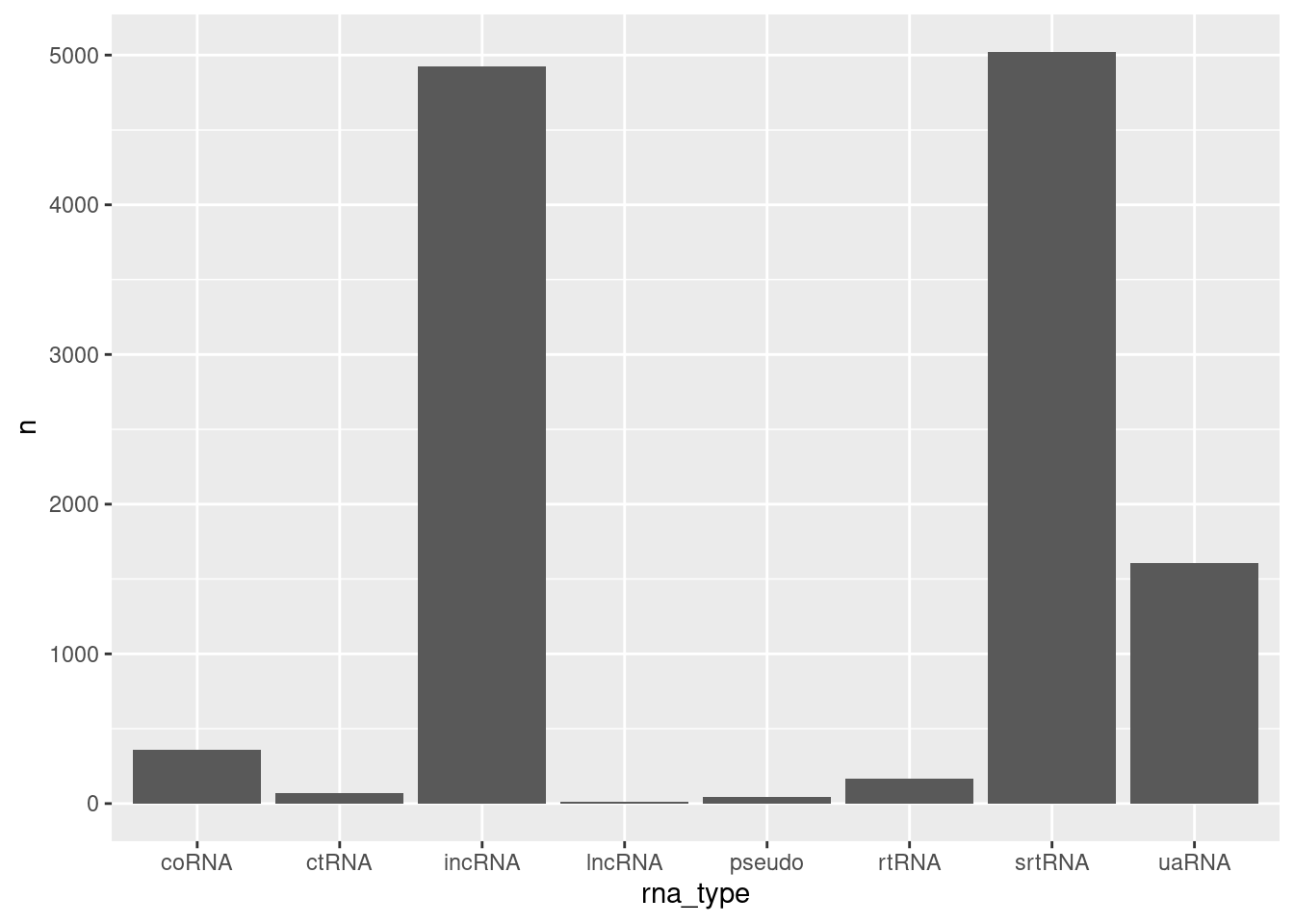

Ok let’s try making that effect size heatmap…

coloc.results.tidycolocalized %>%
  left_join(
    ncRNA.annotations %>%
      mutate(PC = "chRNA.Expression_ncRNA") %>%
      dplyr::select(1,2, PC) %>%
      rename(P=gene_name) %>%
      filter(!str_detect(rna_type, ","))
  ) %>%
  mutate(PC = case_when(
    !is.na(rna_type) ~ rna_type,
    TRUE ~ PC
  )) %>%
  group_by(Locus, snp) %>%
  filter(any(PC=="Expression.Splicing.Subset_YRI") & any(!is.na(rna_type))) %>%
  ungroup() %>%
  filter((PC %in% c("Expression.Splicing.Subset_YRI","H3K27AC", "H3K4ME1", "H3K4ME3")) | (!is.na(rna_type))) %>%
  left_join(., ., by=c("Locus", "snp")) %>%
  filter(!((P.x == P.y) & (PC.x == PC.y))) %>%
  group_by(PC.x, PC.y) %>%
  summarise(cor = cor(beta.x, beta.y, method="spearman"),
            n=n()) %>%
  mutate(PC.x = recode(PC.x, !!!PC.ShortAliases)) %>%
  mutate(PC.y = recode(PC.y, !!!PC.ShortAliases)) %>%
  ggplot(aes(x=PC.x, y=PC.y, fill=cor)) +
  geom_raster() +
  scale_fill_gradient2() +
  geom_text(aes(label=n)) +
  scale_x_discrete(expand=c(0,0)) +
  scale_y_discrete(expand=c(0,0)) +
  theme_classic() +
  theme(axis.text.x = element_text(angle = 45, vjust = 1, hjust=1)) +
  labs(x="TraitA Phenotype class", y="TraitB Phenotype class", fill="Spearman cor", title="Effect size correlation")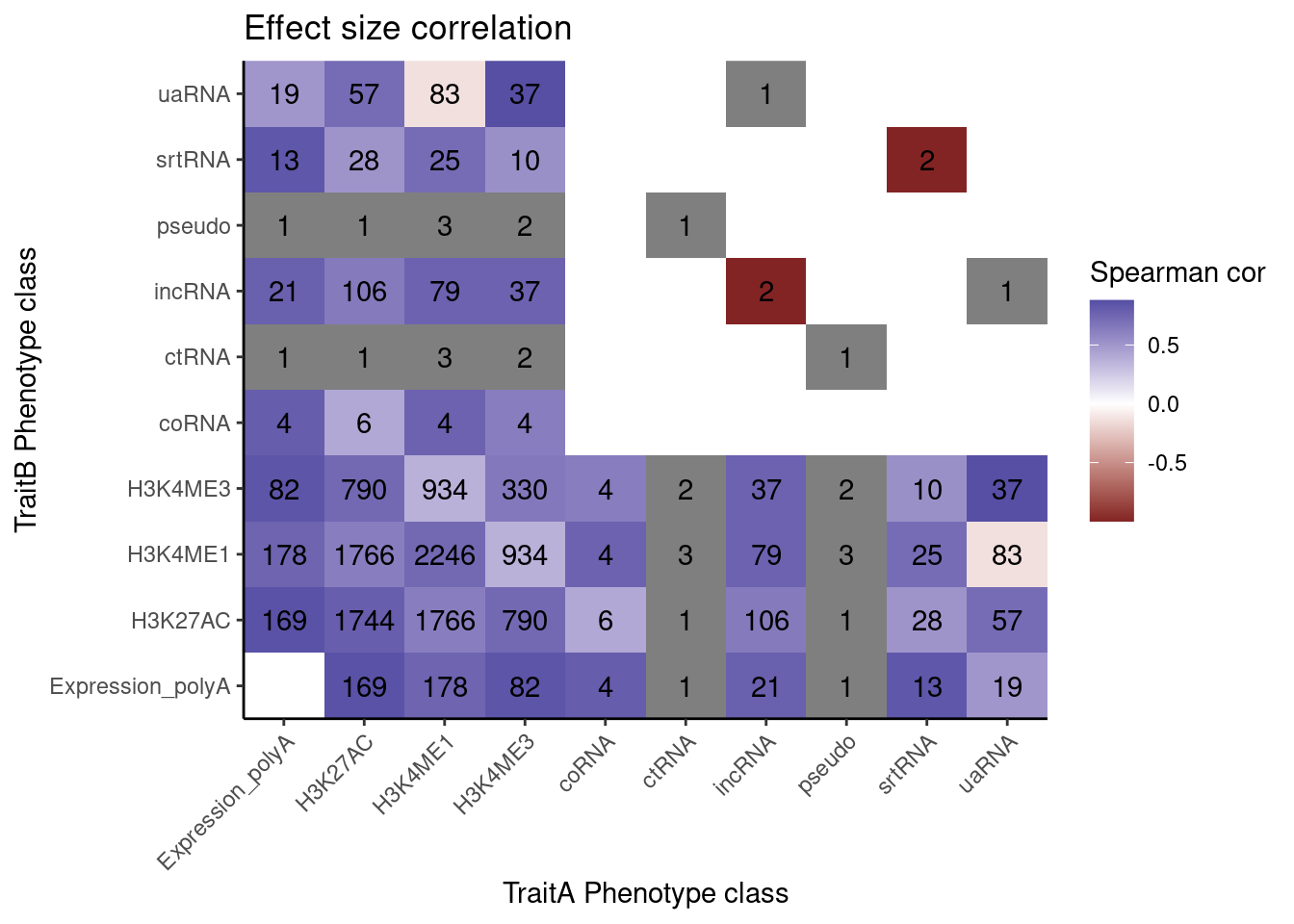

Session information

sessionInfo()

R version 3.6.1 (2019-07-05)
Platform: x86_64-pc-linux-gnu (64-bit)
Running under: CentOS Linux 7 (Core)

Matrix products: default
BLAS/LAPACK: /software/openblas-0.2.19-el7-x86_64/lib/libopenblas_haswellp-r0.2.19.so

locale:
 [1] LC_CTYPE=en_US.UTF-8 LC_NUMERIC=C         LC_TIME=C           
 [4] LC_COLLATE=C         LC_MONETARY=C        LC_MESSAGES=C       
 [7] LC_PAPER=C           LC_NAME=C            LC_ADDRESS=C        
[10] LC_TELEPHONE=C       LC_MEASUREMENT=C     LC_IDENTIFICATION=C 

attached base packages:
[1] stats     graphics  grDevices utils     datasets  methods   base     

other attached packages:
 [1] data.table_1.14.2 forcats_0.4.0     stringr_1.4.0     dplyr_1.0.9      
 [5] purrr_0.3.4       readr_1.3.1       tidyr_1.2.0       tibble_3.1.7     
 [9] ggplot2_3.3.6     tidyverse_1.3.0  

loaded via a namespace (and not attached):
 [1] Rcpp_1.0.5        lubridate_1.7.4   assertthat_0.2.1  rprojroot_2.0.2  
 [5] digest_0.6.20     utf8_1.1.4        R6_2.4.0          cellranger_1.1.0 
 [9] backports_1.4.1   reprex_0.3.0      evaluate_0.15     httr_1.4.4       
[13] highr_0.9         pillar_1.7.0      rlang_1.0.5       readxl_1.3.1     
[17] rstudioapi_0.14   R.oo_1.22.0       R.utils_2.9.0     rmarkdown_1.13   
[21] labeling_0.3      munsell_0.5.0     broom_1.0.0       compiler_3.6.1   
[25] httpuv_1.5.1      modelr_0.1.8      xfun_0.31         pkgconfig_2.0.2  
[29] htmltools_0.5.3   tidyselect_1.1.2  workflowr_1.6.2   fansi_0.4.0      
[33] crayon_1.3.4      dbplyr_1.4.2      withr_2.5.0       later_0.8.0      
[37] R.methodsS3_1.7.1 grid_3.6.1        jsonlite_1.6      gtable_0.3.0     
[41] lifecycle_1.0.1   DBI_1.1.0         git2r_0.26.1      magrittr_1.5     
[45] scales_1.1.0      cli_3.3.0         stringi_1.4.3     farver_2.1.0     
[49] fs_1.5.2          promises_1.0.1    xml2_1.3.2        ellipsis_0.3.2   
[53] generics_0.1.3    vctrs_0.4.1       tools_3.6.1       glue_1.6.2       
[57] hms_0.5.3         fastmap_1.1.0     yaml_2.2.0        colorspace_1.4-1 
[61] rvest_0.3.5       knitr_1.39        haven_2.3.1