CheckQTL_SNPPositionsMetagene

Intro

I will for each class of QTLs, check the SNP positions of significant QTLs, reading in the output from QTLtools permutation pass.

library(tidyverse)
library(data.table)
library(GGally)

PhenotypeAliases <- read_tsv("../data/Phenotypes_recode_for_Plotting.txt")

PermutationPass.dat <- Sys.glob("../code/QTLs/QTLTools/*/PermutationPass.FDR_Added.txt.gz") %>%
  setNames(str_replace(., "../code/QTLs/QTLTools/(.+?)/PermutationPass.FDR_Added.txt.gz", "\\1")) %>%
  lapply(read_delim, delim=' ') %>%
  bind_rows(.id="PhenotypeClass")

First explore the data a bit… count QTLs for example…

NumTestFeats <- PermutationPass.dat %>%
  count(PhenotypeClass)
NumQTLs <- PermutationPass.dat %>%
  filter(q<0.1) %>%
  count(PhenotypeClass)

ggplot(data = NumTestFeats,
         aes(x=PhenotypeClass, y=n)) +
  geom_col() +
  geom_text(aes(label=n), color="black", angle=70, hjust=-0.4, size=2) +
  geom_errorbar(
    data = NumQTLs,
    aes(y = n, ymin = n, ymax = n), color="black",lty=1, size=1.5) +
  geom_text(
    data = NumQTLs,
    aes(y=n, label=n), color="red", angle=90, hjust=-0.4, size=2) +
  scale_y_continuous(trans='log10', limits=c(1,1E6)) +
  theme_classic() +
  theme(axis.text.x = element_text(angle = 45, vjust = 1, hjust=1)) +
  labs(y="Number features/QTLs", caption="Number of test features (black) and QTLs (red); FDR<10%")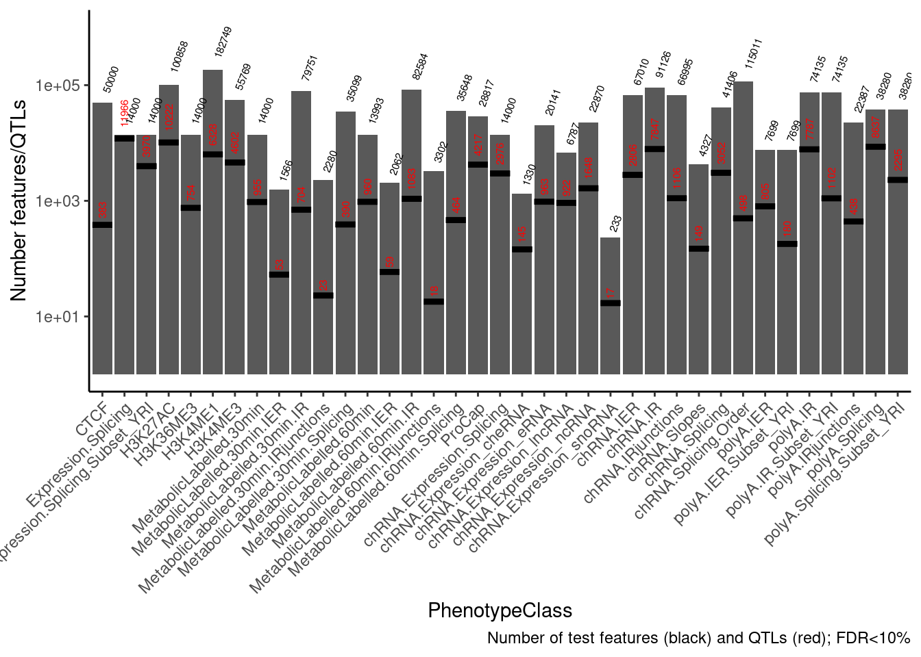

Now plot metaplot of where QTLs in relation to the phenotype. for sQTLs, I used the --group setting for permutation testing for a cluster-level test, though for now (out of convenience) i’m going to plot positions of top SNPs relative to the top intron.

First just plot distances…

First explore the data a bit… are all strands either + or - in a sensible way?

PermutationPass.dat %>%
  count(PhenotypeClass, phe_strd)

# A tibble: 69 × 3
   PhenotypeClass                 phe_strd      n
   <chr>                          <chr>     <int>
 1 CTCF                           +         50000
 2 Expression.Splicing            +          7112
 3 Expression.Splicing            -          6888
 4 Expression.Splicing.Subset_YRI +          7112
 5 Expression.Splicing.Subset_YRI -          6888
 6 H3K27AC                        +        100858
 7 H3K36ME3                       +          7112
 8 H3K36ME3                       -          6888
 9 H3K4ME1                        +        182749
10 H3K4ME3                        +         55769
# … with 59 more rows

Notice the ChIP-seq data should not technically be stranded. Let’s replace those “+” strand entries with “.”…

PermutationPass.dat <- PermutationPass.dat %>%
  mutate(phe_strd = case_when(
     PhenotypeClass %in% c("H3K27AC", "H3K4ME1", "H3K4ME3", "CTCF") ~ ".",
     TRUE ~ phe_strd
  ))

PermutationPass.dat %>%
  count(PhenotypeClass, phe_strd)

# A tibble: 69 × 3
   PhenotypeClass                 phe_strd      n
   <chr>                          <chr>     <int>
 1 CTCF                           .         50000
 2 Expression.Splicing            +          7112
 3 Expression.Splicing            -          6888
 4 Expression.Splicing.Subset_YRI +          7112
 5 Expression.Splicing.Subset_YRI -          6888
 6 H3K27AC                        .        100858
 7 H3K36ME3                       +          7112
 8 H3K36ME3                       -          6888
 9 H3K4ME1                        .        182749
10 H3K4ME3                        .         55769
# … with 59 more rows

Next to make a metaplot we need to decide on some details, specifically on how to plot thing around boundaries… Should we scale all features to the same plot length? Around the edges should we just plot absolute distance (as kilobases)?

Let’s first plot the distribution of feature lengths before further making these decisions…

PermutationPass.dat %>%
  mutate(feat_length = phe_to-phe_from) %>%
  ggplot(aes(x=feat_length)) +
  stat_ecdf() +
  geom_label(
    data = . %>%
      group_by(PhenotypeClass) %>%
      summarise(label = median(feat_length)),
    aes(label=label),
    x=Inf, y=-Inf, size=3, hjust=1, vjust=0) +
  scale_x_continuous(trans='log10') +
  facet_wrap(~PhenotypeClass) +
  theme_bw() +
  labs(caption="feature length. median labelled")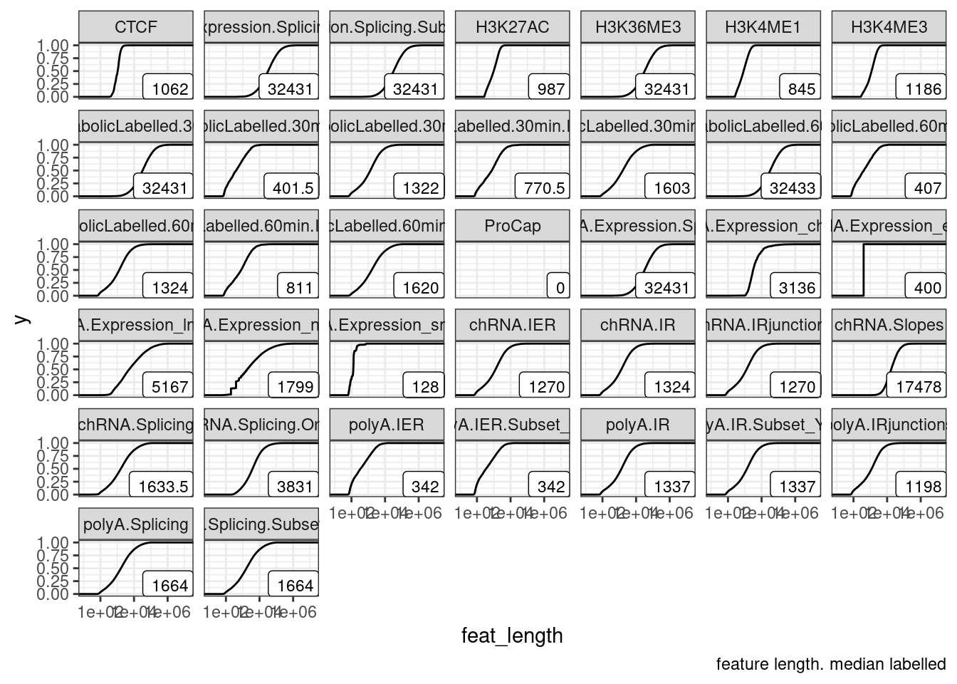

Hm, for now, let’s just focus on making a reasonable metagene plot rather than figuring out the details of how to make reasonable meta-intron, meta-cluster, or meta-ChIP-peak plot (each of which may require different amounts of squeezing to fairly represent distances within the feature versus flanking the feature).

Making metagene plots like this in a reasonable way takes some thought, since features are different sizes so some features get squeezed more than others, while the flanking regions i want to make a set distance (eg, each bin is a contant 1kb). So how many bins to squeeze the middle part into? Let’s try to make the size of the middle bins similarly to the size of the flanking bins, based on the median gene size…

# Determine breaks for `cut`.
## Number of bins for middle part
NumBinsInMiddle <- 20
MedianGeneLength <- 32431

MetaplotBreaks <- c(seq(-50000, 0, MedianGeneLength/NumBinsInMiddle), seq(0,1, length.out=NumBinsInMiddle), rev(seq(50000,1, by=-MedianGeneLength/NumBinsInMiddle)))

PermutationPass.dat %>%
  mutate(feat_length = phe_to-phe_from) %>%
  add_count(PhenotypeClass) %>%
  filter(n < 14001 & n > 13000) %>%
  filter(q<0.1) %>%
  mutate(DistForPlot = case_when(
    #Var within feature
    (phe_strd == "+") & (dist_phe_var == 0) ~ (var_from  - phe_from)/feat_length,
    (phe_strd == "-") & (dist_phe_var == 0) ~ (phe_to  - var_from)/feat_length,
    #Var downstream of feature
    phe_strd == "+" & (var_from > phe_to) ~ var_from - phe_to,
    phe_strd == "-" & (var_from < phe_from) ~ phe_from - var_from,
    #Var upstream of feature
    phe_strd == "+" & (var_from < phe_from) ~ var_from - phe_from,
    phe_strd == "-" & (var_from > phe_to) ~ var_from - phe_to
  )) %>%
  # mutate(RelativeDistForPlot = cut(DistForPlot, breaks=c(-Inf, MetaplotBreaks, Inf))) %>%
  mutate(RelativeDistForPlot = cut(DistForPlot, breaks=c(MetaplotBreaks))) %>%
  filter(!is.na(RelativeDistForPlot)) %>%
  ggplot(aes(x=RelativeDistForPlot)) +
  geom_bar() +
  facet_wrap(~PhenotypeClass, scales = "free_y") +
  theme_classic() +
  theme(axis.text.x = element_text(angle = 90, vjust = 0.5, hjust=1, size=4))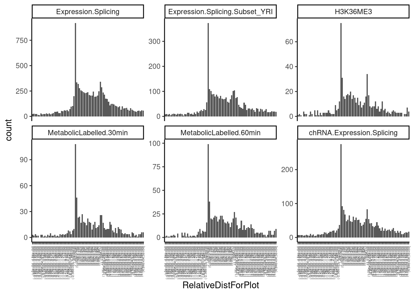

Ok, those look nice and as expected. I think later about making similar plots for introns/sQTLs.

Looking at SNP annotation enrichments

Let’s also look for enrichment for top SNPs (not “finemapped” in any fancy way, just the nominally most significant SNP as output from QTLtools) among genome annotation sets (eg enhancer, promoter, splice site, etc). For each top SNP, I have already intersected it with a list of annotations. Here I will read in that data and explore it…

First let’s read in the annotation region set and explore

annotation.regions <- fread("../code/QTL_SNP_Enrichment/Annotations.bed.gz", sep='\t',col.names=c("chrom", "start", "stop", "category", "name", "strand"))

annotation.regions.lengths <- annotation.regions %>%
  mutate(Length = stop-start) %>%
  group_by(category) %>%
  summarise(Total.length = sum(Length))

annotation.regions.lengths %>%
  mutate(Total.length.M = signif(Total.length/1E6, 3)) %>%
ggplot(aes(x=category, y=Total.length.M, label=Total.length.M)) +
  geom_col(position = "dodge2", color="black") +
    geom_text(angle=90, hjust=-0.1, size=2.5) +
    scale_y_continuous(expand=c(0,0), trans="log10", limits=c(1, 5E4)) +
  theme_classic() +
  theme(axis.text.x = element_text(angle = 45, vjust = 1, hjust=1)) +
  labs(y="Total length of annotationa category\n(Megabases)")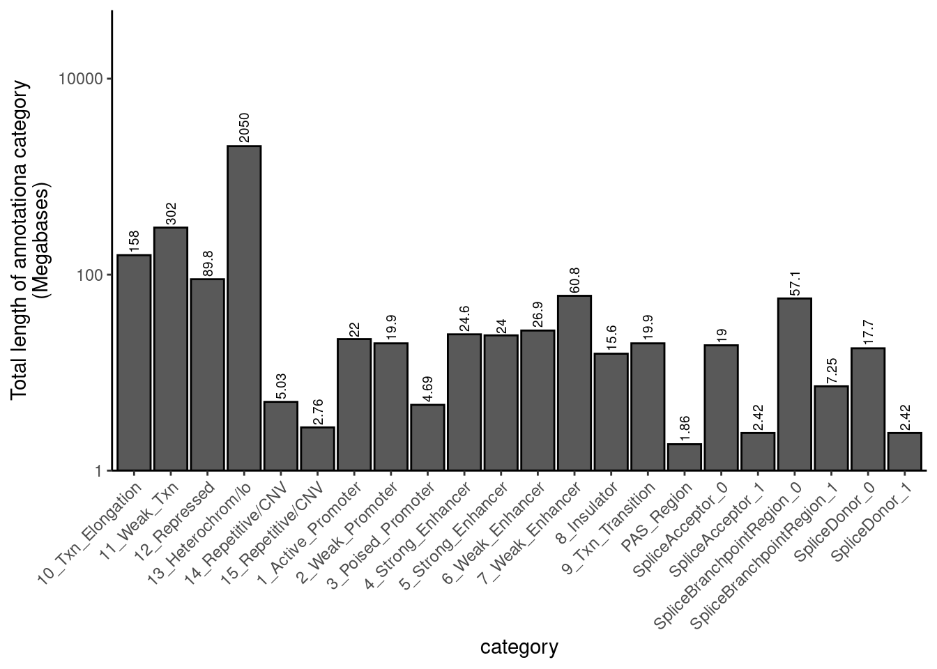

CategoryFactorOrderedLevels <- annotation.regions.lengths %>%
  mutate(ChromHMMCategory = as.numeric(str_extract(category, "^\\d+"))) %>%
  arrange(ChromHMMCategory, category) %>%
  mutate(SuperCategory = case_when(
    str_detect(category,"Splice") ~ "Splicing",
    str_detect(category,"PAS") ~ "PAS",
    str_detect(category,"Enhancer") ~ "Enhancer",
    str_detect(category,"Promoter") ~ "Promoter",
    str_detect(category,"Txn") ~ "Transcribed",
    str_detect(category,"Repetitive") ~ "Repetitive",
    TRUE ~ NA_character_
    ))

Now, let’s calculate an enrichment score just by the number of topSNPs intersecting each category, divided by the total length of the annotation category. This does not control for some things that maybe should be controlled for, like some level of background enrichment for test SNPs (test SNPs will by definition be close/cis to genes). I think the head to head comparisons like I have done previously (ie, comparing relative enrichments of sQTLs versus eQTLs between categories, and using the same gene-wise test SNP windows) should implicitly control for a lot of these things, and I’ll do something like that later. Also, previously I estimated a confidence interval with bootstrap samples. But first let’s just do this more simple enrichment analysis to get a quicker feel for things…

TopSNPs.intersectedWithRegions <- Sys.glob("../code/QTL_SNP_Enrichment/TopSNPIntersections/*.bed.gz") %>%
  setNames(str_replace(., "../code/QTL_SNP_Enrichment/TopSNPIntersections/(.+?).bed.gz", "\\1")) %>%
  lapply(fread, col.names=c("chrom", "start", "stop", "SNP.ID", "gid", "score","p.extras", "annotation.chrom", "annotation.start", "annotation.stop", "category", "basesOverlap")) %>%
  bind_rows(.id="PhenotypeClass") %>%
  dplyr::select(PhenotypeClass, chrom, start, stop, SNP.ID, gid, p.extras, category) %>%
  separate(p.extras, into=c("pid", "p.start", "p.stop", "p.beta", "p.p", "p.q"), convert=T, sep=";")

Simple.EnrichmentScores <- TopSNPs.intersectedWithRegions %>%
  filter(p.q < 0.1) %>%
  add_count(PhenotypeClass) %>%
  count(PhenotypeClass, category, n) %>%
  mutate(FractionSNPsInClass = nn/n) %>%
  left_join(
    annotation.regions.lengths %>%
      mutate(FractionCategoryInGenome = Total.length/sum(Total.length))
    ) %>%
  drop_na() %>%
  mutate(enrichment = FractionSNPsInClass/FractionCategoryInGenome) %>%
  mutate(PhenotypeClass_n = paste0(PhenotypeClass, "(", n, ")")) %>%
  left_join(CategoryFactorOrderedLevels) %>%
  mutate(category = factor(category, levels=CategoryFactorOrderedLevels$category))

ggplot(Simple.EnrichmentScores, aes(y=log2(enrichment), x=category)) +
  geom_col(aes(fill=SuperCategory)) +
  coord_flip() +
  scale_x_discrete(limits=rev) +
  facet_wrap(~PhenotypeClass_n) +
  theme_bw() +
  labs(x="log2(Enrichment)", caption=str_wrap("Enrichment calculated as fraction of TopSNPs in each cateory divided by fraction category in the genome"))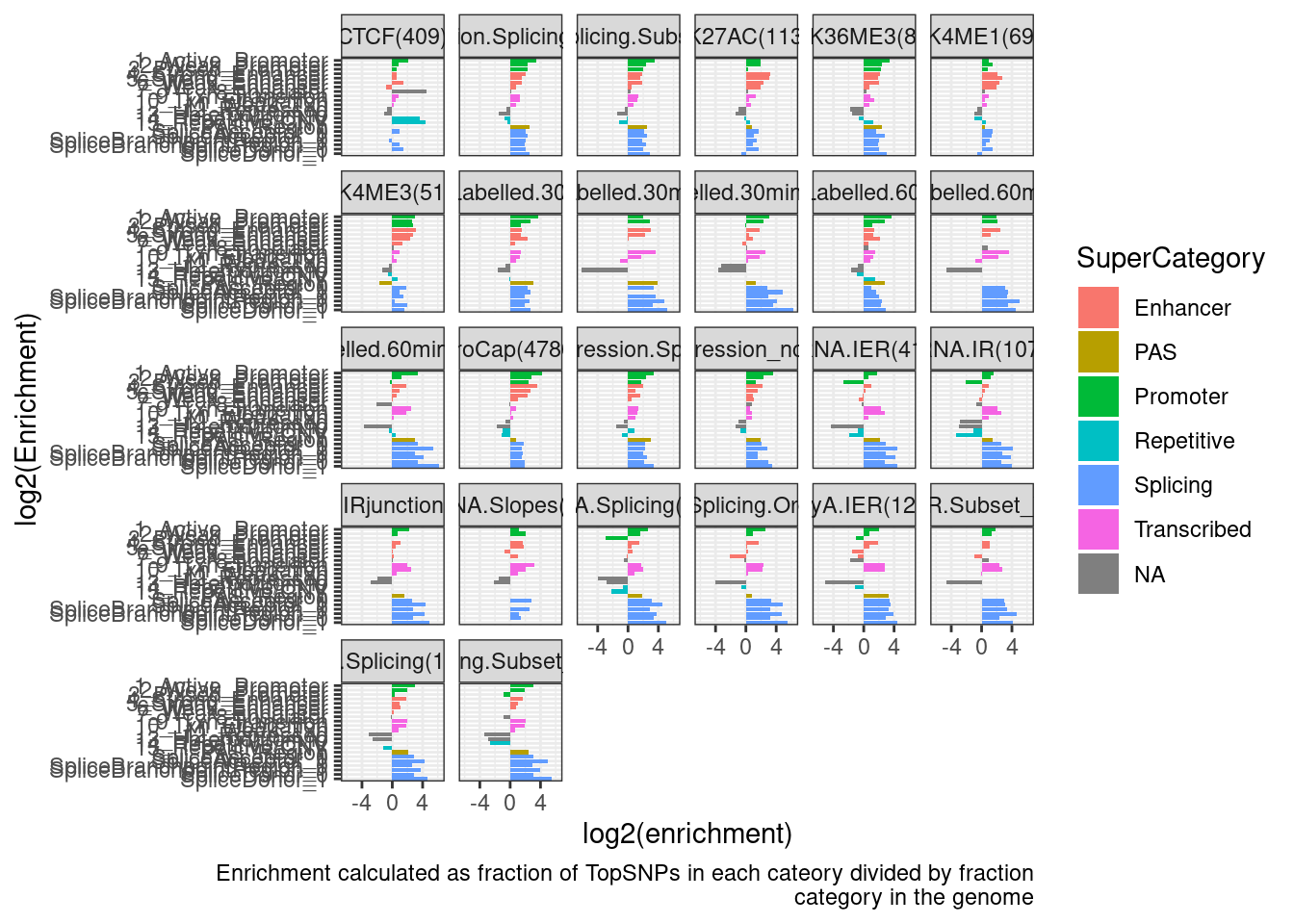

Yeah, this is kind of hard to interpret…

Let’s just focus on a few phenotypes of interest…

Simple.EnrichmentScores %>%
  filter(str_detect(PhenotypeClass, "chRNA")) %>%
  ggplot(aes(y=log2(enrichment), x=category)) +
  geom_col(aes(fill=SuperCategory)) +
  geom_text(aes(label=nn), size=3, color='red') +
  coord_flip() +
  scale_x_discrete(limits=rev) +
  facet_wrap(~PhenotypeClass_n) +
  theme_bw() +
  labs(x="log2(Enrichment)", caption=str_wrap("Enrichment calculated as fraction of TopSNPs in each cateory divided by fraction category in the genome. Numbers of QTLs in each category labelelled"))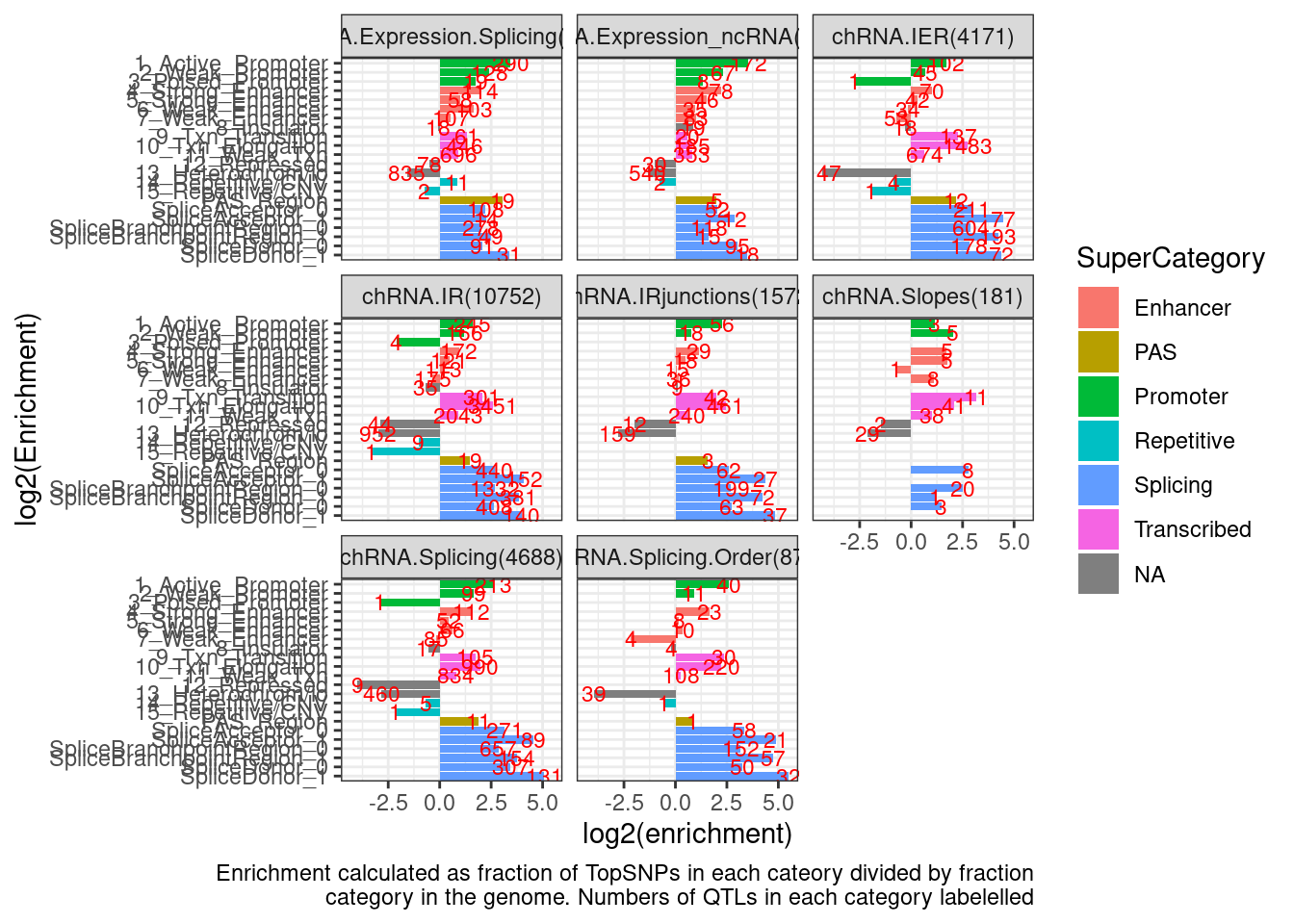

But I do see some notable things, like sQTLs enriched in splice sites compared to eQTLs. Let’s go back to doing head to head comparisons and making confidence intervals.

Different metrics for intron retention

3 methods: - IR.juncs: fraction of spliced junction reads out of splice+unspliced junction reads (splice-q) - IER: “Intron excision ratio”, ratio of intronic coverage over exonic coverage (splice-q) - IR: Ratio of intronic coverage to gene-wise median exonic coverage:

Let’s explore the p-val correlation for the three methods

diag_limitrange <- function(data, mapping, ...) { 
  ggplot(data = data, mapping = mapping, ...) + 
    geom_density(...) + 
    theme_bw()
}

upper_point <- function(data, mapping, ...) { 
  ggplot(data = data, mapping = mapping, ...) + 
    geom_point(..., alpha=0.05) + 
    geom_abline() +
    theme_bw()
}

qq <- function(data, mapping, ...) { 
  ggplot(data = data, mapping = mapping, ...) + 
    geom_point(aes(y=-log10(1-percent_rank(mapping)))) + 
    theme_bw()
}



PermutationPass.dat %>%
  filter(PhenotypeClass %in% c("chRNA.IER", "chRNA.IRjunctions", "chRNA.IR")) %>%
  ggplot(aes(x=adj_beta_pval)) +
  geom_histogram() +
  facet_wrap(~PhenotypeClass) +
  theme_bw() +
  labs(title="histogram of permutation pass P")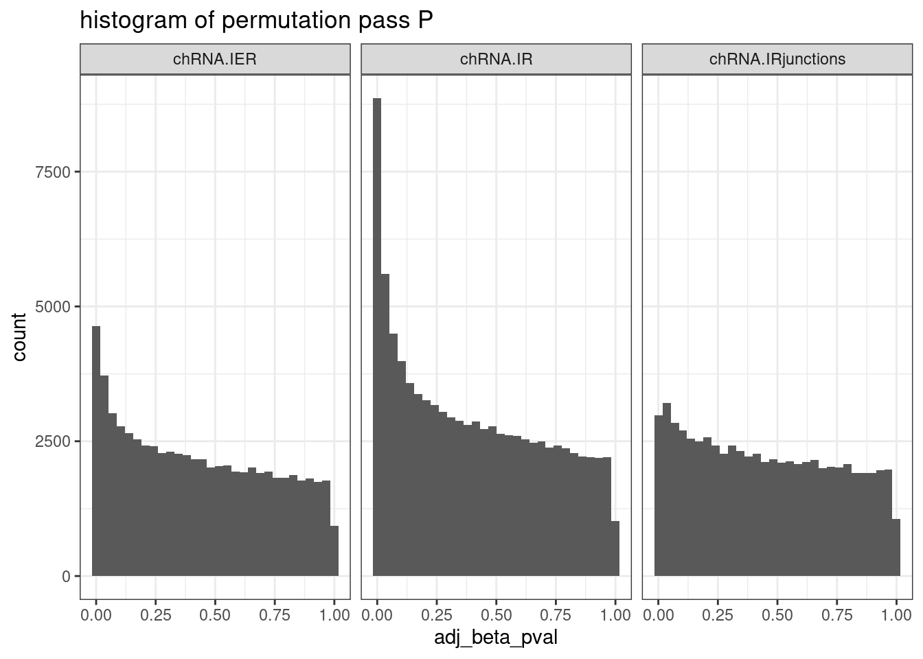

PermutationPass.dat$PhenotypeClass %>% unique()

 [1] "CTCF"                                "Expression.Splicing.Subset_YRI"     
 [3] "Expression.Splicing"                 "H3K27AC"                            
 [5] "H3K36ME3"                            "H3K4ME1"                            
 [7] "H3K4ME3"                             "MetabolicLabelled.30min.IER"        
 [9] "MetabolicLabelled.30min.IR"          "MetabolicLabelled.30min.IRjunctions"
[11] "MetabolicLabelled.30min.Splicing"    "MetabolicLabelled.30min"            
[13] "MetabolicLabelled.60min.IER"         "MetabolicLabelled.60min.IR"         
[15] "MetabolicLabelled.60min.IRjunctions" "MetabolicLabelled.60min.Splicing"   
[17] "MetabolicLabelled.60min"             "ProCap"                             
[19] "chRNA.Expression.Splicing"           "chRNA.Expression_cheRNA"            
[21] "chRNA.Expression_eRNA"               "chRNA.Expression_lncRNA"            
[23] "chRNA.Expression_ncRNA"              "chRNA.Expression_snoRNA"            
[25] "chRNA.IER"                           "chRNA.IR"                           
[27] "chRNA.IRjunctions"                   "chRNA.Slopes"                       
[29] "chRNA.Splicing.Order"                "chRNA.Splicing"                     
[31] "polyA.IER.Subset_YRI"                "polyA.IER"                          
[33] "polyA.IR.Subset_YRI"                 "polyA.IR"                           
[35] "polyA.IRjunctions"                   "polyA.Splicing.Subset_YRI"          
[37] "polyA.Splicing"                     

PermutationPass.dat %>%
  filter(PhenotypeClass=="chRNA.IR")

# A tibble: 91,126 × 25
   PhenotypeClass phe_id      phe_chr phe_from phe_to phe_strd n_var_in_cis
   <chr>          <chr>       <chr>      <dbl>  <dbl> <chr>           <dbl>
 1 chRNA.IR       IntID.52863 chr1      944804 945038 -                 173
 2 chRNA.IR       IntID.52986 chr1      945426 945514 -                 167
 3 chRNA.IR       IntID.53017 chr1      945657 946169 -                 167
 4 chRNA.IR       IntID.53078 chr1      946290 946398 -                 161
 5 chRNA.IR       IntID.53261 chr1      948236 948486 -                 156
 6 chRNA.IR       IntID.53340 chr1      948607 951123 -                 167
 7 chRNA.IR       IntID.53829 chr1      951242 951996 -                 152
 8 chRNA.IR       IntID.53899 chr1      952143 952408 -                 152
 9 chRNA.IR       IntID.53951 chr1      952604 953171 -                 153
10 chRNA.IR       IntID.54005 chr1      953292 953778 -                 153
# … with 91,116 more rows, and 18 more variables: dist_phe_var <dbl>,
#   var_id <chr>, var_chr <chr>, var_from <dbl>, var_to <dbl>, dof1 <dbl>,
#   dof2 <dbl>, bml1 <dbl>, bml2 <dbl>, nom_pval <dbl>, r_squared <dbl>,
#   slope <dbl>, slope_se <dbl>, adj_emp_pval <dbl>, adj_beta_pval <dbl>,
#   q <dbl>, grp_id <chr>, n_phe_in_grp <dbl>

P.dat <-PermutationPass.dat %>%
  filter(PhenotypeClass %in% c("chRNA.IER", "chRNA.IRjunctions", "chRNA.IR")) %>%
  dplyr::select(phe_id:phe_strd, PhenotypeClass, adj_beta_pval) %>%
  mutate(LogP = -log10(adj_beta_pval)) %>%
  pivot_wider(names_from = "PhenotypeClass", values_from = "LogP", id_cols=phe_chr:phe_strd) %>%
  dplyr::select(chRNA.IER, chRNA.IR, chRNA.IRjunctions)

P <- ggpairs(P.dat,
    # upper=list(continuous = my_fn),
    upper=list(continuous = wrap("cor", method = "spearman", hjust=0.7)),
    lower=list(continuous = upper_point),
    diag=list(continuous = "blankDiag")) +
  theme_classic()
  


SymetricMatrixLabels <- colnames(P.dat)
for (i in seq_along(SymetricMatrixLabels)){
    ToPlotForQQ <- P.dat %>%
        select(SymetricMatrixLabels[i]) %>%
        rename("LogP"=1) %>%
        mutate(ExpectedLogP = -log10(1-percent_rank(LogP)))
    P[i,i] <- ggplot(ToPlotForQQ) +
        geom_point(aes(x=ExpectedLogP, y=LogP)) +
        geom_abline()
        theme_bw() +
        theme(
        panel.grid.major.y = element_blank(),
        panel.grid.minor.y = element_blank()
        # axis.text.x = element_text(angle = 45, vjust = 0.5, hjust=1)
        )
}

P +
  labs("Comparing Pvals from three intron-retention quantification methods")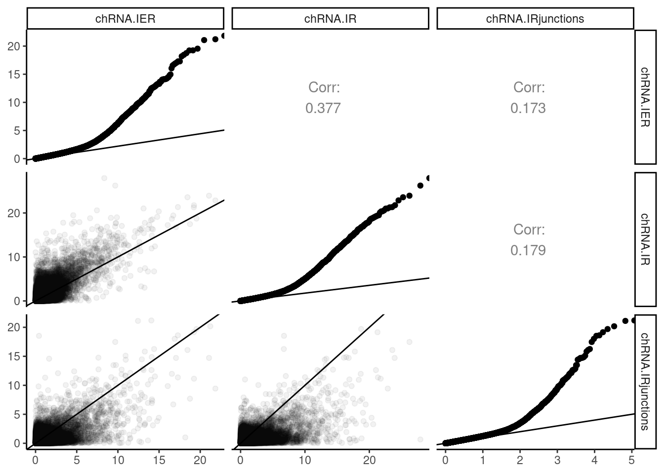

PermutationPass.dat %>%
  filter(PhenotypeClass %in% c("chRNA.IER", "chRNA.IRjunctions", "chRNA.IR")) %>%
  dplyr::select(phe_id:phe_strd, var_id, PhenotypeClass, q, slope) %>%
  pivot_wider(names_from = "PhenotypeClass", values_from = c("q", "slope"), id_cols=phe_chr:var_id) %>%
  drop_na() %>%
  filter(q_chRNA.IR < 0.1) %>%
  dplyr::select(contains("slope")) %>%
  ggpairs() +
  theme_bw()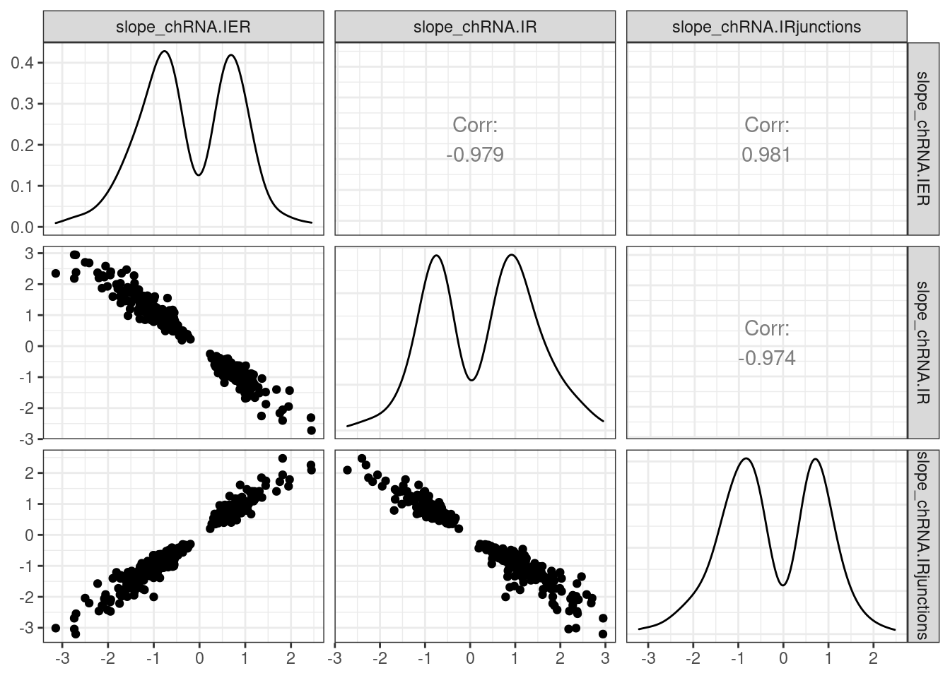

Ok, this verifies that I coded the chRNA.IR phenotype in such a way that a bigger number means more intron retention. The other metrics, IER and IR.junctions, are reversed so that a bigger number means less intron retention. Also, given the really high overlap between QTLs called using these different methods, it is clear to me that the previously observed effect of lots of intron retention QTLs with same direction effects as eQTL (more intron retention coinciding with higher exonic-gene expression) will not go away no matter which of the three methods I use. Yet, all of these three phenotypes are enriched for splice sites, about to a similar degree as standard leafcutter sQTLs. I should more carefully investigate this phenomena about intron retention and direction of effects…

Session information

sessionInfo()

R version 3.6.1 (2019-07-05)
Platform: x86_64-pc-linux-gnu (64-bit)
Running under: CentOS Linux 7 (Core)

Matrix products: default
BLAS/LAPACK: /software/openblas-0.2.19-el7-x86_64/lib/libopenblas_haswellp-r0.2.19.so

locale:
 [1] LC_CTYPE=en_US.UTF-8 LC_NUMERIC=C         LC_TIME=C           
 [4] LC_COLLATE=C         LC_MONETARY=C        LC_MESSAGES=C       
 [7] LC_PAPER=C           LC_NAME=C            LC_ADDRESS=C        
[10] LC_TELEPHONE=C       LC_MEASUREMENT=C     LC_IDENTIFICATION=C 

attached base packages:
[1] stats     graphics  grDevices utils     datasets  methods   base     

other attached packages:
 [1] GGally_1.4.0      data.table_1.14.2 forcats_0.4.0     stringr_1.4.0    
 [5] dplyr_1.0.9       purrr_0.3.4       readr_1.3.1       tidyr_1.2.0      
 [9] tibble_3.1.7      ggplot2_3.3.6     tidyverse_1.3.0  

loaded via a namespace (and not attached):
 [1] Rcpp_1.0.5         lubridate_1.7.4    assertthat_0.2.1   rprojroot_2.0.2   
 [5] digest_0.6.20      utf8_1.1.4         R6_2.4.0           cellranger_1.1.0  
 [9] plyr_1.8.4         backports_1.4.1    reprex_0.3.0       evaluate_0.15     
[13] highr_0.9          httr_1.4.4         pillar_1.7.0       rlang_1.0.5       
[17] readxl_1.3.1       rstudioapi_0.14    R.oo_1.22.0        R.utils_2.9.0     
[21] rmarkdown_1.13     labeling_0.3       munsell_0.5.0      broom_1.0.0       
[25] compiler_3.6.1     httpuv_1.5.1       modelr_0.1.8       xfun_0.31         
[29] pkgconfig_2.0.2    htmltools_0.5.3    tidyselect_1.1.2   workflowr_1.6.2   
[33] reshape_0.8.8      fansi_0.4.0        crayon_1.3.4       dbplyr_1.4.2      
[37] withr_2.5.0        later_0.8.0        R.methodsS3_1.7.1  grid_3.6.1        
[41] jsonlite_1.6       gtable_0.3.0       lifecycle_1.0.1    DBI_1.1.0         
[45] git2r_0.26.1       magrittr_1.5       scales_1.1.0       cli_3.3.0         
[49] stringi_1.4.3      farver_2.1.0       fs_1.5.2           promises_1.0.1    
[53] xml2_1.3.2         ellipsis_0.3.2     generics_0.1.3     vctrs_0.4.1       
[57] RColorBrewer_1.1-2 tools_3.6.1        glue_1.6.2         hms_0.5.3         
[61] fastmap_1.1.0      yaml_2.2.0         colorspace_1.4-1   rvest_0.3.5       
[65] knitr_1.39         haven_2.3.1