H3K4me3FromGruber
Last updated: 2020-08-21
Checks: 5 1
Knit directory: ChromatinSplicingQTLs/analysis/
This reproducible R Markdown analysis was created with workflowr (version 1.6.2). The Checks tab describes the reproducibility checks that were applied when the results were created. The Past versions tab lists the development history.
Great job! The global environment was empty. Objects defined in the global environment can affect the analysis in your R Markdown file in unknown ways. For reproduciblity it’s best to always run the code in an empty environment.
The command set.seed(20191126) was run prior to running the code in the R Markdown file. Setting a seed ensures that any results that rely on randomness, e.g. subsampling or permutations, are reproducible.
Great job! Recording the operating system, R version, and package versions is critical for reproducibility.
Nice! There were no cached chunks for this analysis, so you can be confident that you successfully produced the results during this run.
Great job! Using relative paths to the files within your workflowr project makes it easier to run your code on other machines.
Tracking code development and connecting the code version to the results is critical for reproducibility. To start using Git, open the Terminal and type git init in your project directory.
This project is not being versioned with Git. To obtain the full reproducibility benefits of using workflowr, please see ?wflow_start.
Introduction
This analysis is an example to demonstrate how I will set up Rmarkdowns for this project. See about for more description. In this example I will make a QQ-plot of H3K4me3 P-values (from Gruber et al), grouped by whether the SNP is an eQTL ( GEUVADIS data ). In the code directory, the snakemake has already downloaded and or processed the data from these publications. I expect that SNPs that are eQTLs will have smaller P-values for H3K4me3.
First load necessary libraries and read in data…
library(tidyverse)── Attaching packages ────────────────────────────────────────────────────── tidyverse 1.3.0 ──✔ ggplot2 3.2.1 ✔ purrr 0.3.4
✔ tibble 2.1.3 ✔ dplyr 0.8.3
✔ tidyr 1.1.0 ✔ stringr 1.4.0
✔ readr 1.3.1 ✔ forcats 0.4.0── Conflicts ───────────────────────────────────────────────────────── tidyverse_conflicts() ──
✖ dplyr::filter() masks stats::filter()
✖ dplyr::lag() masks stats::lag()library(knitr)
Grubert.H3K4me3.QTLs <- read.delim("../code/PlotGruberQTLs/Data/localQTLs_H3K4ME3.FDR0.1.hg38.bedpe", col.names=c("SNP_chr", "SNP_pos", "SNP_stop", "Peak_Chr", "Peak_start", "Peak_stop", "Name", "Score", "strand1", "stand2"), stringsAsFactors = F) %>%
separate(col = "Name", into=c("PEAKid","SNPrsid","beta","p.value","FDR_TH","pvalTH","pass.pvalTH","mod","peak.state"), sep = ";", convert = T) %>%
mutate(SNP_pos = as.numeric(SNP_pos))
head(Grubert.H3K4me3.QTLs) %>% kable()| SNP_chr | SNP_pos | SNP_stop | Peak_Chr | Peak_start | Peak_stop | PEAKid | SNPrsid | beta | p.value | FDR_TH | pvalTH | pass.pvalTH | mod | peak.state | Score | strand1 | stand2 |
|---|---|---|---|---|---|---|---|---|---|---|---|---|---|---|---|---|---|
| chr10 | 98266058 | 98266059 | chr10 | 98267895 | 98268846 | 1 | rs10748723 | 0.2032748 | 0.2292467 | 0.1 | 0.0009998 | fail | H3K4ME3 | TSS | . | . | . |
| chr10 | 98268012 | 98268013 | chr10 | 98267895 | 98268846 | 1 | rs10786407 | -0.1114408 | 0.6567359 | 0.1 | 0.0009998 | fail | H3K4ME3 | TSS | . | . | . |
| chr10 | 98268054 | 98268055 | chr10 | 98267895 | 98268846 | 1 | rs10883055 | -0.1188379 | 0.6095054 | 0.1 | 0.0009998 | fail | H3K4ME3 | TSS | . | . | . |
| chr10 | 98266369 | 98266370 | chr10 | 98267895 | 98268846 | 1 | rs11189529 | -0.6061942 | 0.0009072 | 0.1 | 0.0009998 | pass | H3K4ME3 | TSS | . | . | . |
| chr10 | 98266356 | 98266357 | chr10 | 98267895 | 98268846 | 1 | rs114440225 | -0.2236145 | 0.5527621 | 0.1 | 0.0009998 | fail | H3K4ME3 | TSS | . | . | . |
| chr10 | 98269803 | 98269804 | chr10 | 98267895 | 98268846 | 1 | rs1325500 | -0.5212768 | 0.0047903 | 0.1 | 0.0009998 | fail | H3K4ME3 | TSS | . | . | . |
GEUVADIS.eQTLs <- read.delim("../data/QTLBase.GEUVADIS.eQTLs.hg38.txt.gz", stringsAsFactors = F) %>%
  mutate(SNP_chr=paste0("chr",SNP_chr)) %>%
  filter(!SNP_chr == "chr6") %>% #blunt way to filter out MHC locus
  mutate(SNP_pos = as.numeric(SNP_pos))  %>%
  mutate(SNP=paste(SNP_chr, SNP_pos))

head(GEUVADIS.eQTLs) %>% kable()| SNP_chr | SNP_pos | Mapped_gene | Trait_chr | Trait_start | Trait_end | Pvalue | Sourceid | SNP |
|---|---|---|---|---|---|---|---|---|
| chr4 | 76939335 | NAAA | 4 | 76834813 | 76862166 | 0.0e+00 | 418 | chr4 76939335 |
| chr4 | 76939335 | CXCL10 | 4 | 76942271 | 76944650 | 0.0e+00 | 418 | chr4 76939335 |
| chr4 | 144902942 | GYPE | 4 | 144792017 | 144826716 | 0.0e+00 | 418 | chr4 144902942 |
| chr4 | 83899764 | SCD5 | 4 | 83550692 | 83719949 | 0.0e+00 | 418 | chr4 83899764 |
| chr4 | 88310523 | HSD17B11 | 4 | 88257667 | 88312340 | 3.1e-06 | 418 | chr4 88310523 |
| chr4 | 84144189 | PLAC8 | 4 | 84011201 | 84058228 | 1.0e-07 | 418 | chr4 84144189 |
Peruse data a little.
hist(Grubert.H3K4me3.QTLs$p.value)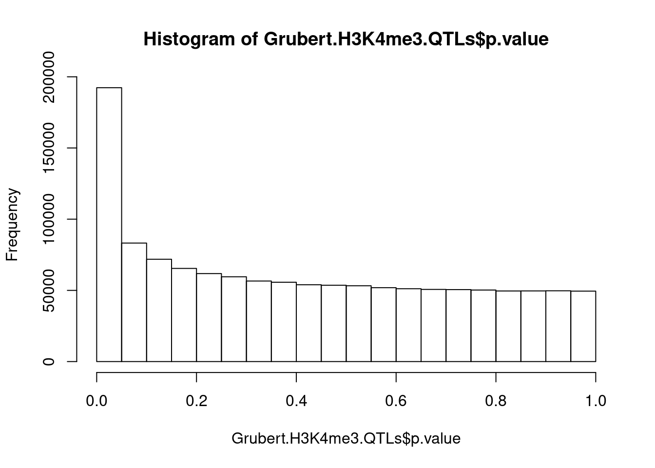
Ok, good look histogram of P-values for H3K4me3 QTLs. What about eQTLs from GEUVADIS which I downlaoded from QTLbase
hist(GEUVADIS.eQTLs$Pvalue)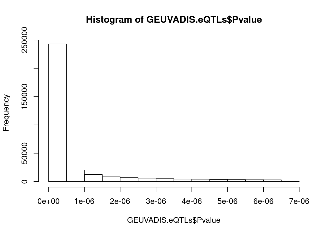
Ok.. those P-values are all very very small. It seems the P values from QTLbase are only for significant eQTLs. So now let’s make a QQ-plot for H3K4me3 QTL P-values, based on whether the snp is an eQTL.
H3K4me3_QQ <- Grubert.H3K4me3.QTLs %>%
  dplyr::select(p.value, SNP_chr, SNP_chr, SNP_pos) %>%
  filter(!SNP_chr == "chr6") %>%
  mutate(SNP=paste(SNP_chr, SNP_pos)) %>%
  mutate(SNPIsEqtl= SNP %in% GEUVADIS.eQTLs$SNP) %>%
  group_by(SNPIsEqtl) %>%
  mutate(ExpectedP=percent_rank(p.value)) %>%
  sample_n(400) %>% #Just sample 400 random points from each group to be quick
  ggplot(aes(x=-log10(ExpectedP), y=-log10(p.value), color=SNPIsEqtl)) +
  geom_point() +
  geom_abline() +
  theme_bw()
H3K4me3_QQ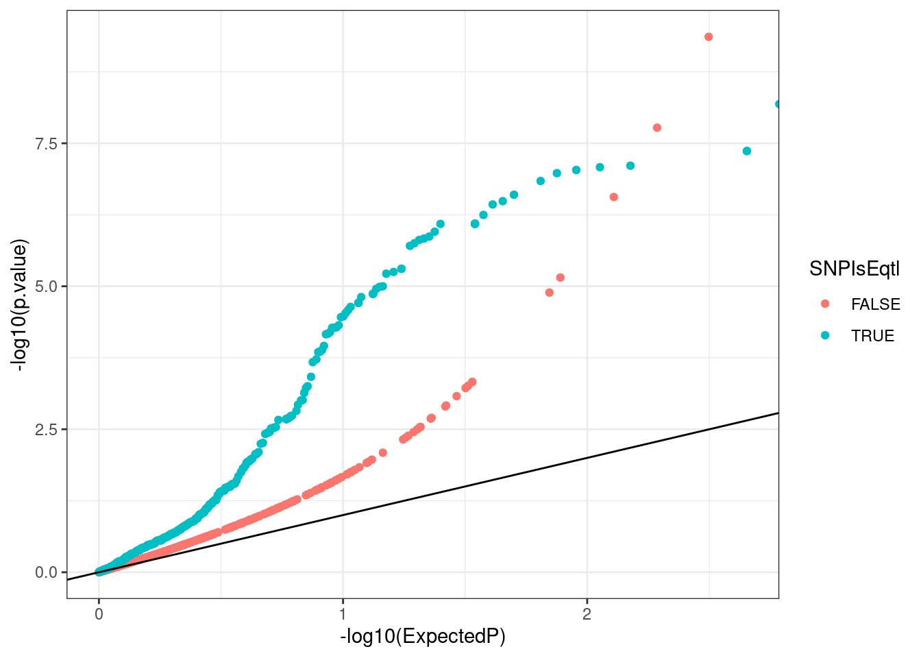
As expected, SNPs that are eQTLs have more significant P-value inflation for H3K4me3 genetic effects.
sessionInfo()R version 3.6.1 (2019-07-05)
Platform: x86_64-pc-linux-gnu (64-bit)
Running under: Scientific Linux 7.4 (Nitrogen)
Matrix products: default
BLAS/LAPACK: /software/openblas-0.2.19-el7-x86_64/lib/libopenblas_haswellp-r0.2.19.so
locale:
[1] LC_CTYPE=en_US.UTF-8 LC_NUMERIC=C
[3] LC_TIME=en_US.UTF-8 LC_COLLATE=en_US.UTF-8
[5] LC_MONETARY=en_US.UTF-8 LC_MESSAGES=en_US.UTF-8
[7] LC_PAPER=en_US.UTF-8 LC_NAME=C
[9] LC_ADDRESS=C LC_TELEPHONE=C
[11] LC_MEASUREMENT=en_US.UTF-8 LC_IDENTIFICATION=C
attached base packages:
[1] stats graphics grDevices utils datasets methods base
other attached packages:
[1] knitr_1.23 forcats_0.4.0 stringr_1.4.0 dplyr_0.8.3
[5] purrr_0.3.4 readr_1.3.1 tidyr_1.1.0 tibble_2.1.3
[9] ggplot2_3.2.1 tidyverse_1.3.0
loaded via a namespace (and not attached):
[1] tidyselect_1.1.0 xfun_0.8 haven_2.3.1 lattice_0.20-38
[5] colorspace_1.4-1 vctrs_0.3.1 generics_0.0.2 htmltools_0.3.6
[9] yaml_2.2.0 rlang_0.4.6 later_0.8.0 pillar_1.4.2
[13] withr_2.1.2 glue_1.3.1 DBI_1.1.0 dbplyr_1.4.2
[17] modelr_0.1.8 readxl_1.3.1 lifecycle_0.1.0 munsell_0.5.0
[21] gtable_0.3.0 workflowr_1.6.2 cellranger_1.1.0 rvest_0.3.5
[25] evaluate_0.14 labeling_0.3 httpuv_1.5.1 highr_0.8
[29] broom_0.5.2 Rcpp_1.0.3 promises_1.0.1 backports_1.1.4
[33] scales_1.1.0 jsonlite_1.6 farver_2.0.1 fs_1.3.1
[37] hms_0.5.3 digest_0.6.20 stringi_1.4.3 grid_3.6.1
[41] rprojroot_1.3-2 cli_1.1.0 tools_3.6.1 magrittr_1.5
[45] lazyeval_0.2.2 crayon_1.3.4 pkgconfig_2.0.2 ellipsis_0.2.0.1
[49] xml2_1.3.2 reprex_0.3.0 lubridate_1.7.4 rstudioapi_0.10
[53] assertthat_0.2.1 rmarkdown_1.13 httr_1.4.1 R6_2.4.0
[57] nlme_3.1-140 git2r_0.26.1 compiler_3.6.1