CheckTehranchiConcordance

Intro

Tehranchi et al used pooled chip-seq assay on YRI LCLs to assess allele-specific binding QTLs for 5 transcription factors. They found that the QTL SNPs over TF motif hits were largely concordant with predicted TF-binding effects from position weight matrix. In our data, I want to check how TF binding may effect other processes, like splicing, for which NFKB for example was recently shown to affect. To do this, first I downloaded TableS2 from Tehranchi et al, lifted over the QTL variants to hg38, searched for TF motif hits (motifs downloaded from JASPAR) for both alleles, and caculated the change in PWM score. I did this all using a script in the snakemake, and in this notebook I will explore the results…

library(tidyverse)
library(qvalue)

dat <- read_tsv("../code/scratch/ScanTFBS.txt.gz")

head(dat)

# A tibble: 6 x 9
  chrom  start   stop TF          P motif  Delta MaxAnyValue
  <chr>  <dbl>  <dbl> <chr>   <dbl> <chr>  <dbl>       <dbl>
1 chr1  777808 777809 NF-kB 0.0210  MA01…  11.0         6.85
2 chr1  777808 777809 PU.1  0.00763 MA01…  11.0         6.85
3 chr1  777809 777810 PU.1  0.00763 MA01…  15.2         6.85
4 chr1  922659 922660 Pou2… 0.0333  MA01…  -5.72       13.0 
5 chr1  922659 922660 Pou2… 0.0333  MA01… -12.8        14.5 
6 chr1  992360 992361 PU.1  0.0135  MA01…  12.1         4.01
# … with 1 more variable: hg38refIsHighbind <lgl>

dat$motif %>% unique()

 [1] "MA0105.4.NFKB1"  "MA0137.2.STAT1"  "MA0137.3.STAT1" 
 [4] "MA0778.1.NFKB2"  "MA0080.2.SPI1"   "MA0105.3.NFKB1" 
 [7] "MA0491.2.JUND"   "MA0105.2.NFKB1"  "MA0492.1.JUND"  
[10] "MA0785.1.POU2F1"

dat$TF %>% unique()

[1] "NF-kB"   "PU.1"    "Pou2f1"  "JunD"    "H3K4me3" "Stat1"  

Each row is a Tehranchi QTL with a TF PWM motif hit. Note that for each QTL, I searched across 10 different JASPAR motifs, since some of the different TF’s that were probed had more than one motif that I thought would be worthwhile checking. One of the first things I should do is condense SNPs for the best hit for the motifs for a single TF, and also select only the direct binding hits (where the QTL TF matches the motif TF)

MotifToTF <- c("MA0105.4.NFKB1"="NF-kB",
               "MA0137.2.STAT1"="Stat1",
               "MA0137.3.STAT1"="Stat1",
               "MA0778.1.NFKB2"="NF-kB",
               "MA0080.2.SPI1"="PU.1",
               "MA0105.3.NFKB1"="NF-kB",
               "MA0491.2.JUND"="JunD",
               "MA0785.1.POU2F1"="Pou2f1"
               )

dat.filtered <- dat %>%
  mutate(motif = recode(motif, !!!MotifToTF)) %>%
  filter(TF == motif) %>%
  group_by(chrom, start, TF) %>%
  arrange(desc(MaxAnyValue)) %>%
  distinct(chrom, start, TF, .keep_all = T) %>%
  ungroup()

The P values here are what is reported in TableS2 from Tehranchi. I think they are nominal P-values, and filtered for nominal Pvalue < 0.05.

dat.filtered$P %>% hist()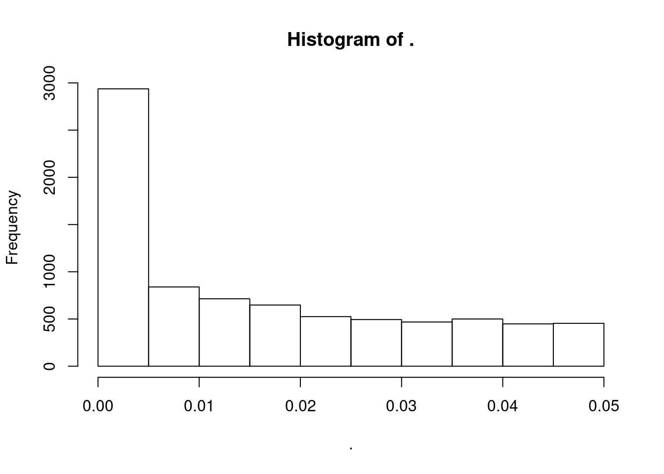

Based on the histogram, most of these QTLs are probably false positives, most of the Pvalue distribution mass is in a flat region. If we had the whole distribution of P-values it would be trivial to estimate FDR and filter out most of the false discoveries.

For now, let’s plot the concordance of deltaPWM (ref-alt) versus if the high binding allele was the ref by plotting histograms of the deltaPWM, colored by if TableS2 reports the the reference (lifted to hg38) is the high binding allele. So I would expect most of the true QTLs with a positive deltaPWM to also be where reference is the high binding allele.

dat.filtered %>%
  filter(!Delta==0) %>%
  ggplot(aes(x=Delta, fill=hg38refIsHighbind)) +
  geom_histogram() +
  facet_wrap(~TF, scales = "free") +
  theme_classic()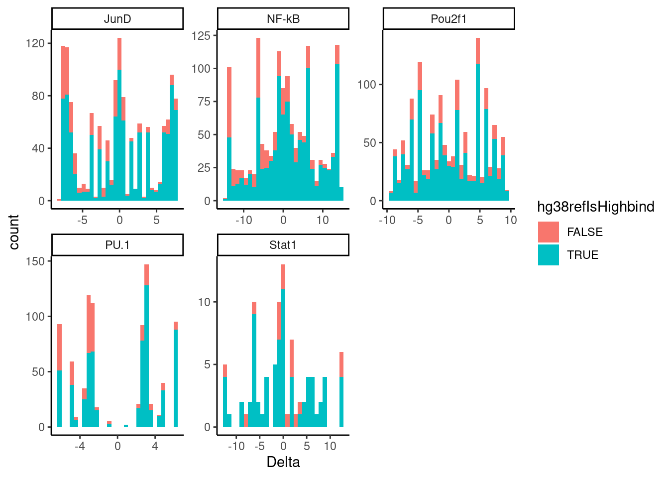

Not much concordance… But what happens if i use a more stringent Pvalue filter to filter out some of the false discoveries…

dat.filtered %>%
  filter(!Delta==0) %>%
  filter(P<0.001) %>%
  ggplot(aes(x=Delta, fill=hg38refIsHighbind)) +
  geom_histogram() +
  facet_wrap(~TF, scales = "free") +
  theme_classic()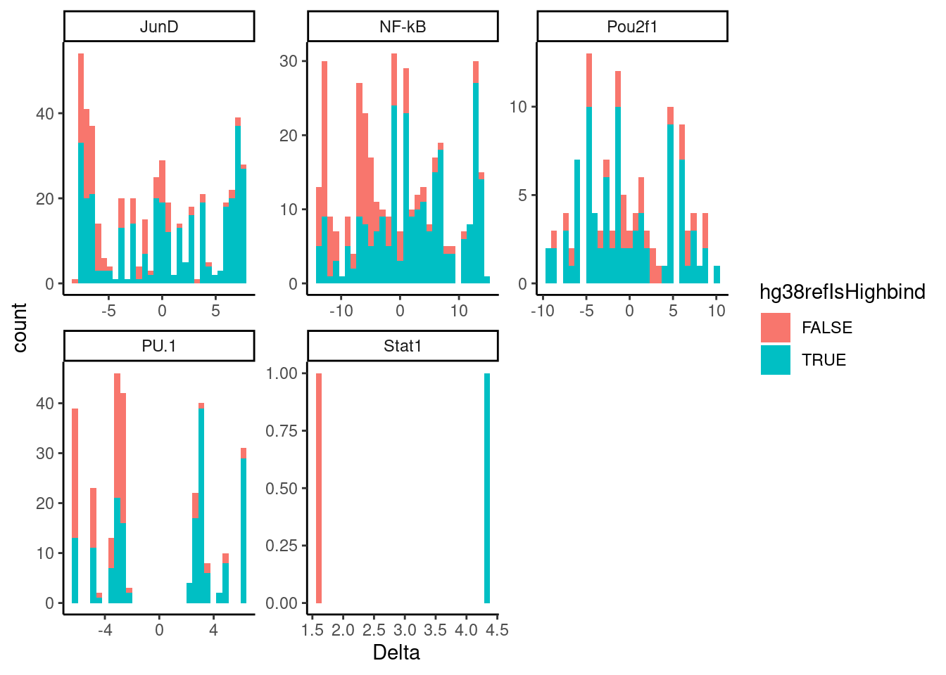

Ok this is a bit more believable. Maybe I should try estimating a FDR and filtering on an appropriate FDR threshold. First let’s plot the Pvalue distribition (at least up to 0.05) for each TF

dat.filtered %>%
  ggplot(aes(x=P)) +
  geom_histogram() +
  facet_wrap(~TF, scales = "free") +
  theme_classic()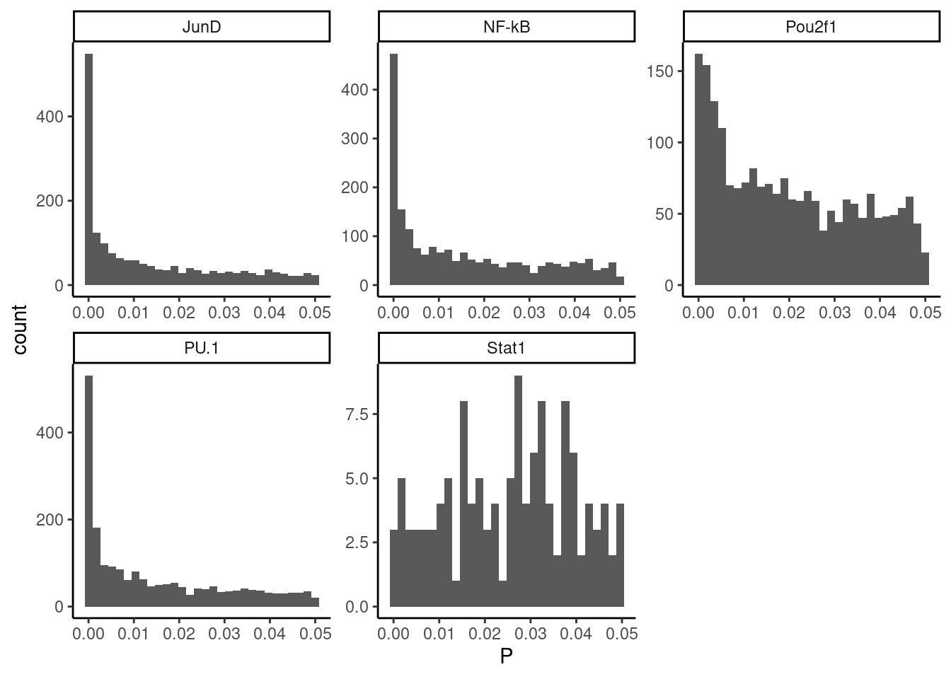

Ok I think I should just drop STAT1 from analysis, and for the others I will try to apply Storey’s q value FDR estimation approach somehow. How about we count the number of observations from 0.04 to 0.05 (mostly flat region, representing 1% of the interval from 0-1), then create 95X as many observations sampled randomly from uniform (from 0.05 to 1) to fill in the rest of the Pvalue distribution with these mock data. Then we can use qvalue package to estimate FDR.

MockPValsToFillIn <- dat.filtered %>%
  filter(!TF == "Stat1") %>%
  filter(P<0.05 & P>0.04) %>%
  select(TF) %>%
  uncount(95) %>%
  mutate(P = runif(nrow(.), 0.05, 1))

#Plot histogram with mock pvalues filled in
dat.filtered %>%
  filter(!TF == "Stat1") %>%
  bind_rows(MockPValsToFillIn) %>%
  ggplot(aes(x=P)) +
  geom_histogram() +
  facet_wrap(~TF, scales = "free") +
  theme_classic()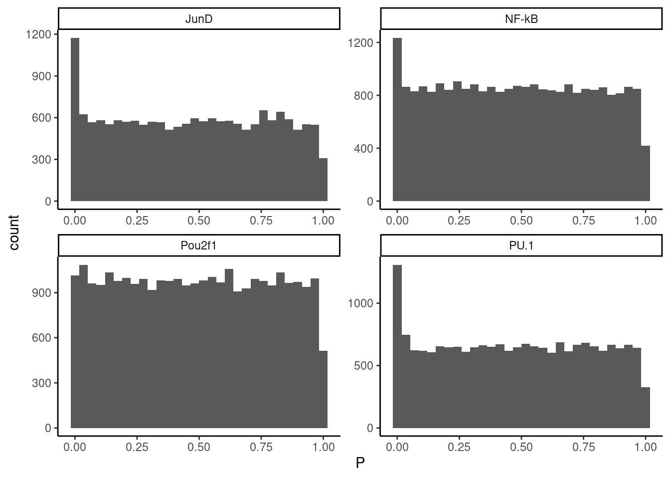

dat.filted.with.FDR <- dat.filtered %>%
  filter(!TF == "Stat1") %>%
  bind_rows(MockPValsToFillIn) %>%
  group_by(TF) %>%
  mutate(q = qvalue(P)$qvalues) %>%
  ungroup()

# Plot qvalues per TF.  Based on the histogram, Pou2f1 should have basically no QTLs that pass a stringent (10%) FDR threshold
dat.filted.with.FDR %>%
  ggplot(aes(x=q)) +
  geom_histogram() +
  facet_wrap(~TF, scales = "free") +
  theme_classic()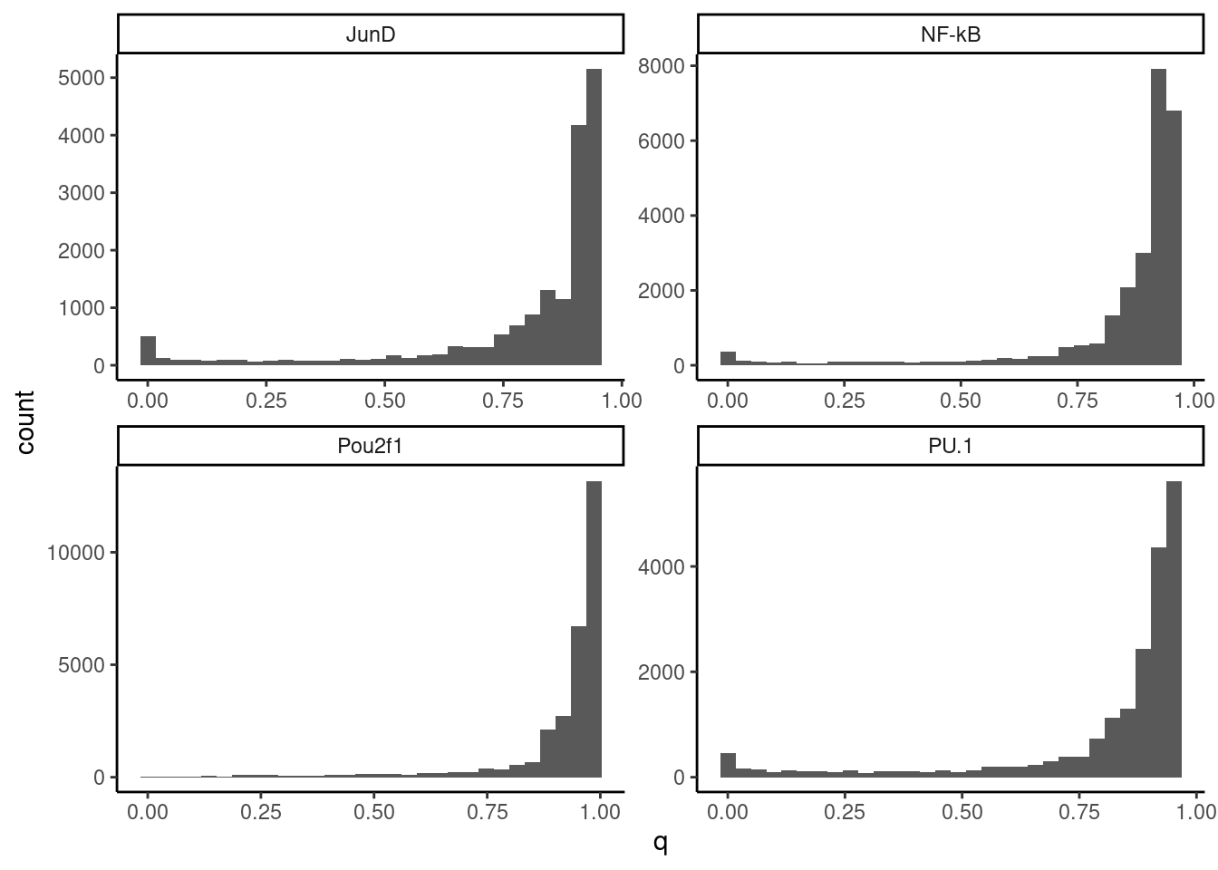

Ok great. I think that worked fine. Now let’s replot the concordance of deltaPWM versus observed high binding allele for FDR10% QTLs

dat.filted.with.FDR %>%
  filter(q < 0.1) %>%
  filter(!Delta==0) %>%
  ggplot(aes(x=Delta, fill=hg38refIsHighbind)) +
  geom_histogram() +
  facet_wrap(~TF, scales = "free") +
  theme_classic()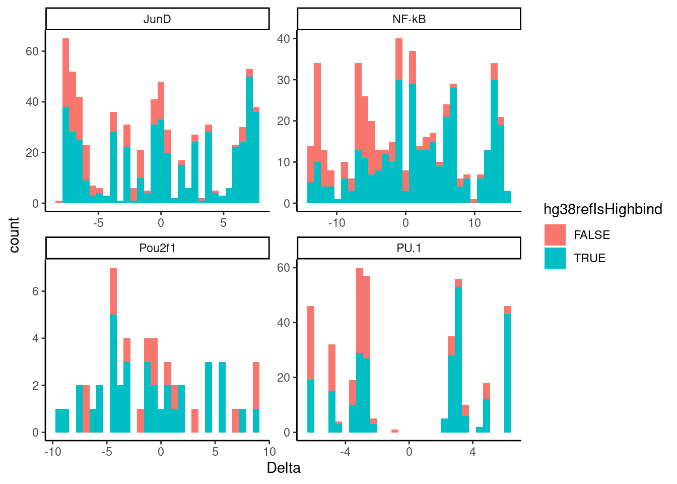

Ok that looks better. Let’s replot a different way, for simplicity:

dat.filted.with.FDR %>%
  filter(q < 0.1) %>%
  filter(!Delta==0) %>%
  mutate(IsRefenceAlleleHigherPWM = Delta>0) %>%
  count(IsRefenceAlleleHigherPWM, hg38refIsHighbind, TF) %>%
  ggplot(aes(x=IsRefenceAlleleHigherPWM, y=n, fill=hg38refIsHighbind)) +
  geom_col() +
  facet_wrap(~TF, scales = "free") +
  labs(x="Is RefAllele higher predicted binding (PWM)", y="Number TF-binding QTLs", fill="Is RefAllele higher observed binding") +
  theme_classic()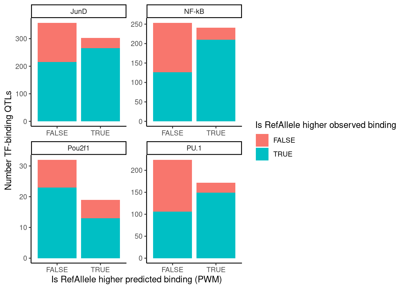

Most of the Pou2f1 might still be false positives, and there weren’t that many QTLs for that TF to begin with… Let’s just drop that from futher analysis. and in general there may still be some bias towards reference allele, perhaps due to mapping biases or something of the sort… But I think I am still picking up on a little signal in that when the referenceAllele has a higher PWM, it is more likely the higher binding allele. Let’s write out these TF QTLs to a new file, and consider quantifying splicing in-around these TF sites.

dat.filted.with.FDR %>%
  filter(!TF == "Pou2f1") %>%
  filter(q < 0.1) %>%
  filter(!Delta==0) %>%
  select(chrom, start, stop, DeltaPWM=Delta, P, TF) %>%
  arrange(chrom, start, stop) %>%
  write_tsv("../data/Tehranchi_PrimaryTFBinding-QTLs.bed.gz")

Session information

sessionInfo()

R version 3.6.1 (2019-07-05)
Platform: x86_64-pc-linux-gnu (64-bit)
Running under: Scientific Linux 7.4 (Nitrogen)

Matrix products: default
BLAS/LAPACK: /software/openblas-0.2.19-el7-x86_64/lib/libopenblas_haswellp-r0.2.19.so

locale:
 [1] LC_CTYPE=en_US.UTF-8       LC_NUMERIC=C              
 [3] LC_TIME=en_US.UTF-8        LC_COLLATE=en_US.UTF-8    
 [5] LC_MONETARY=en_US.UTF-8    LC_MESSAGES=en_US.UTF-8   
 [7] LC_PAPER=en_US.UTF-8       LC_NAME=C                 
 [9] LC_ADDRESS=C               LC_TELEPHONE=C            
[11] LC_MEASUREMENT=en_US.UTF-8 LC_IDENTIFICATION=C       

attached base packages:
[1] stats     graphics  grDevices utils     datasets  methods   base     

other attached packages:
 [1] qvalue_2.16.0   forcats_0.4.0   stringr_1.4.0   dplyr_0.8.3    
 [5] purrr_0.3.4     readr_1.3.1     tidyr_1.1.0     tibble_2.1.3   
 [9] ggplot2_3.3.5   tidyverse_1.3.0

loaded via a namespace (and not attached):
 [1] tidyselect_1.1.0 xfun_0.8         reshape2_1.4.3   splines_3.6.1   
 [5] haven_2.3.1      lattice_0.20-38  colorspace_1.4-1 vctrs_0.3.1     
 [9] generics_0.0.2   htmltools_0.3.6  yaml_2.2.0       utf8_1.1.4      
[13] rlang_0.4.10     later_0.8.0      pillar_1.4.2     withr_2.4.1     
[17] glue_1.3.1       DBI_1.1.0        dbplyr_1.4.2     modelr_0.1.8    
[21] readxl_1.3.1     plyr_1.8.4       lifecycle_0.1.0  munsell_0.5.0   
[25] gtable_0.3.0     workflowr_1.6.2  cellranger_1.1.0 rvest_0.3.5     
[29] evaluate_0.14    labeling_0.3     knitr_1.23       httpuv_1.5.1    
[33] fansi_0.4.0      broom_0.5.2      Rcpp_1.0.5       promises_1.0.1  
[37] backports_1.1.4  scales_1.1.0     jsonlite_1.6     farver_2.1.0    
[41] fs_1.3.1         hms_0.5.3        digest_0.6.20    stringi_1.4.3   
[45] grid_3.6.1       rprojroot_2.0.2  cli_2.2.0        tools_3.6.1     
[49] magrittr_1.5     crayon_1.3.4     pkgconfig_2.0.2  xml2_1.3.2      
[53] reprex_0.3.0     lubridate_1.7.4  rstudioapi_0.10  assertthat_0.2.1
[57] rmarkdown_1.13   httr_1.4.1       R6_2.4.0         nlme_3.1-140    
[61] git2r_0.26.1     compiler_3.6.1