Introduction

I’ve been making heatmaps to communicate the fraction of xQTLs (eg eQTLs/sQTLs/chromatinQTLs) that colocalize with yQTLs. There are many slightly different methods I’ve been using to make this heatmap, with slightly different interpretations. In this notebook, I will make lots of those heatmaps to compare the different methods.

Here is a list of the different methods I have been using, with the names I am calling these methods. Note that for all of these methods I can consider using different statistical thresholds for calling something a QTL, so in this notebook I’ll explore that too.

• Pi1: “What is the pi1 statistic for yQTLs (ascertainment phenotype), in xQTLs (discovery phenotype)”. I can use different FDR thresholds for x (discovery phenotype)
• ColocalizationRate: “What fraction of xQTLs have at least one colocalizing yQTL”.
• ColocalizationRateAmongAttempted: “When there is both a xQTL and yQTL around the same gene, how often do they colocalize”
• SpearmanCorrealtionThreshold: What fraction of xQTLs have at least one yQTL with correlated association signal (spearman correlation coef > Treshold)
• SpearmanCorrealtionThresholdAmongAttempted: When there is both a xQTL and yQTL around the same gene, how often do they have correlation association signals (spearman correlation coef > Treshold)

library(tidyverse)
library(viridis)
library(gplots)
library(data.table)
library(qvalue)
library(purrr)
library(GGally)
library(pROC)

# pi0est function breaks sometimes. this wrapper function returns 1 when that happens
CalculatePi1 <- function (dat.in, ...) {
  return(tryCatch(1-pi0est(dat.in$Pvals.For.Pi1, ...)$pi0, error=function(e) 1))
}

pi1

First let’s read in data for Pi1 method

FilesChunks <- paste0("../code/scratch/PairwisePi1Traits.P.", 1:10, ".txt.gz")


dat <- lapply(FilesChunks, fread, sep='\t') %>%
  bind_rows()

RecodeDat <- read_tsv("../data/Phenotypes_recode_for_Plotting.txt")

RecodeVec <- RecodeDat %>%
  select(PC, ShorterAlias) %>%
  deframe()

RecodeIncludePCs <- RecodeDat %>%
  filter(Include) %>%
  pull(PC)

colnames(dat)

 [1] "PC1"                      "P1"                      
 [3] "GeneLocus"                "p_permutation.x"         
 [5] "singletrait_topvar.x"     "singletrait_topvar_chr.x"
 [7] "singletrait_topvar_pos.x" "FDR.x"                   
 [9] "PC2"                      "P2"                      
[11] "p_permutation.y"          "singletrait_topvar.y"    
[13] "singletrait_topvar_chr.y" "singletrait_topvar_pos.y"
[15] "FDR.y"                    "trait.x.p.in.y"          

I also need to simulate the null distribution to deal with the one to many problem…

MaxSampleSizeToCreateANull <- 250
NSamplesToEstimateDistribution <- 10000
NullSimulatedTestStats <- matrix(nrow=MaxSampleSizeToCreateANull, ncol=NSamplesToEstimateDistribution)
rownames(NullSimulatedTestStats) <- paste0("runif_samplesize", 1:MaxSampleSizeToCreateANull)
colnames(NullSimulatedTestStats) <- paste0("Sample_", 1:NSamplesToEstimateDistribution)


for (i in 1:MaxSampleSizeToCreateANull){
  SampleSizeFromUniform <- i
  SampledDat <- matrix(runif(SampleSizeFromUniform*NSamplesToEstimateDistribution), nrow=NSamplesToEstimateDistribution)
  SampleDatNullTestStatistics <- -log10(apply(SampledDat, 1, min))
  NullSimulatedTestStats[i,] <- SampleDatNullTestStatistics
}


NullSimulatedTestStats %>%
  as.data.frame() %>%
  rownames_to_column("runif_samplesize") %>%
  slice(1:20) %>%
  # mutate(runif_samplesize = as.numeric(str_remove(runif_samplesize, "runif_samplesize"))) %>%
  gather(key="Sample", value="value", -runif_samplesize) %>%
  ggplot(aes(x=value, color=runif_samplesize)) +
  geom_density() +
  theme_bw()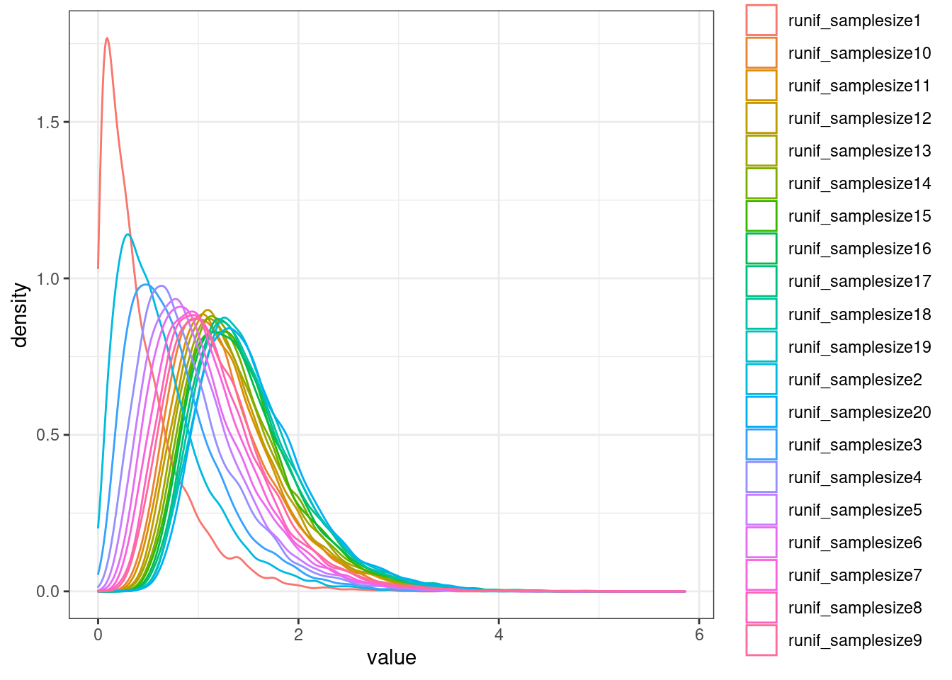

ecdf.functions <- apply(NullSimulatedTestStats, 1, ecdf)
ecdf.functions[[1]](1)

[1] 0.9036

Now calculate pi1

dat.split <- dat %>%
  filter(PC1 %in% RecodeIncludePCs) %>%
  filter(PC2 %in% RecodeIncludePCs) %>%
  mutate(PC1 = recode(PC1, !!!RecodeVec)) %>%
  mutate(PC2 = recode(PC2, !!!RecodeVec)) %>%
  group_by(PC1, P1, PC2) %>%
  mutate(test.stat.obs = -log10(min(trait.x.p.in.y))) %>%
  ungroup() %>%
  add_count(PC1, P1, PC2) %>%
  filter(n<=100) %>%
  group_by(PC1, PC2) %>%
  rowwise() %>%
  mutate(Pvals.For.Pi1 = 1-ecdf.functions[[n]](test.stat.obs)) %>%
  ungroup() %>%
  select(PC1, PC2, Pvals.For.Pi1) %>%
  filter(!PC1==PC2) %>%
  split(paste(.$PC1, .$PC2, sep = ";"))

dat.pi1 <- lapply(dat.split, CalculatePi1) %>%
  unlist() %>%
  data.frame(pi1=.) %>%
  rownames_to_column("PC1_PC2") %>%
  separate(PC1_PC2, into=c("PC1", "PC2"), sep=';')

pi.heatmap <- ggplot(dat.pi1, aes(x=PC1, y=PC2, fill=pi1)) +
  geom_raster() +
  geom_text(aes(label=signif(pi1*100, 2)), color="blue") +
  scale_fill_viridis(option="A", direction = -1, limits=c(0,1)) +
  coord_flip() +
  theme_classic() +
  theme(axis.text.x = element_text(angle = 90, vjust = 0.5, hjust=1)) +
  labs(x="Discovery QTL phenotype", y="Phenotype assessed for overlap")
pi.heatmap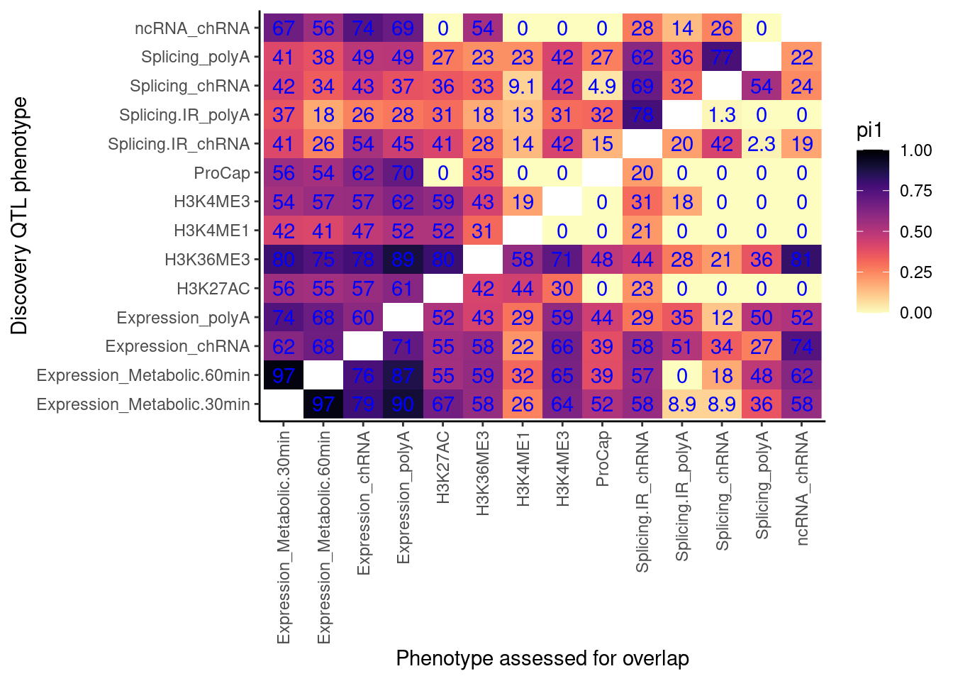 

Ok, there are some 0 values… Let’s check the P value distribution as histogram for these cells in the heatmap to see what’s up with pi1 estimation…

dat.split %>%
  bind_rows(.id="ID") %>%
  # filter(PC1 == "ProCap" & PC2 == "H3K4ME3") %>%
  ggplot(aes(x=Pvals.For.Pi1)) +
  geom_histogram() +
  facet_wrap(~ID, scales = "free_y") +
  theme_bw()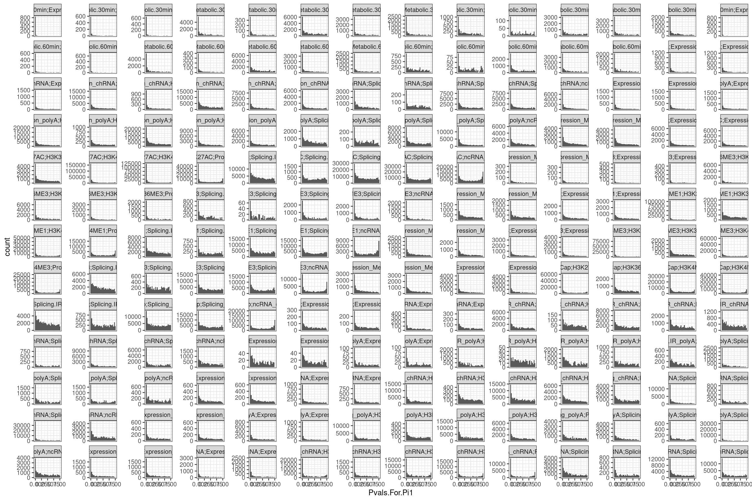

Ok by in large the p value histograms look good. let’s zoom in on one of the problematic histograms.

dat.split %>%
  bind_rows(.id="ID") %>%
  filter(PC1 == "ProCap" & PC2 == "H3K4ME3") %>%
  pull(Pvals.For.Pi1) %>%
  hist(breaks=100)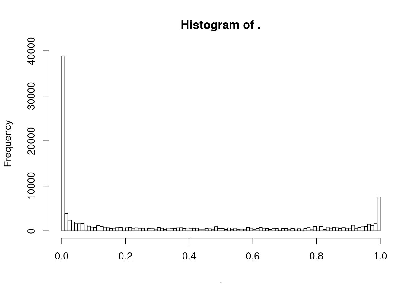

Ok, I could see how pi0est function might have trouble with this histogram. Let’s play with the methods parameter to see how it effects things.

dat.split %>%
  bind_rows(.id="ID") %>%
  filter(PC1 == "ProCap" & PC2 == "H3K4ME3") %>%
  pull(Pvals.For.Pi1) %>%
  pi0est(pi0.method="smoother")

$pi0
[1] 1

$pi0.lambda
 [1] 0.6268863 0.6020165 0.5937425 0.5969455 0.6001775 0.6078990 0.6177524
 [8] 0.6269954 0.6424722 0.6605468 0.6846282 0.7169067 0.7496413 0.8149586
[15] 0.8954897 0.9921968 1.1268392 1.4137042 2.1635114

$lambda
 [1] 0.05 0.10 0.15 0.20 0.25 0.30 0.35 0.40 0.45 0.50 0.55 0.60 0.65 0.70 0.75
[16] 0.80 0.85 0.90 0.95

$pi0.smooth
 [1] 0.5694685 0.5696858 0.5704027 0.5723214 0.5763434 0.5835632 0.5952669
 [8] 0.6129310 0.6382021 0.6728370 0.7186174 0.7772207 0.8500475 0.9380003
[15] 1.0412060 1.1588122 1.2888099 1.4278979 1.5716760

dat.split %>%
  bind_rows(.id="ID") %>%
  filter(PC1 == "ProCap" & PC2 == "H3K4ME3") %>%
  pull(Pvals.For.Pi1) %>%
  pi0est(pi0.method="bootstrap")

$pi0
[1] 0.6001775

$pi0.lambda
 [1] 0.6268863 0.6020165 0.5937425 0.5969455 0.6001775 0.6078990 0.6177524
 [8] 0.6269954 0.6424722 0.6605468 0.6846282 0.7169067 0.7496413 0.8149586
[15] 0.8954897 0.9921968 1.1268392 1.4137042 2.1635114

$lambda
 [1] 0.05 0.10 0.15 0.20 0.25 0.30 0.35 0.40 0.45 0.50 0.55 0.60 0.65 0.70 0.75
[16] 0.80 0.85 0.90 0.95

$pi0.smooth
NULL

Ok I think the key is to use the pi0.method="bootstrap" parameter for the pi0est function. That seems to yield pi0 estimations that are more in line with what I would estimate by eye from the histogram. This publication has some detials on the difference between these two methods for estimating \(\pi_0\). My understanding in brief, is that the ‘smooth’ method uses spline fitting to estimate the \(\lambda\) parameter which defines exactly what p-value to define as 100% null tests, and the p-values less than \(\lambda\) are a mixture of null and non-null tests. If \(\lambda\) is over-estimated, then pi0 will be downwardly biased, however, it is a bias/variance tradeoff… So the smoothing fits a smooth curve to estimate \(\lambda\), assuming the the p-value distribution has the least mass at 1 (thereby making the \(\pi_0\) very sensitive to fluctuations at the right edge of the P-value histogram), whereas the bootstrap method randomly samples from the P-value vector to find an optimal balance between variance and bias for estimating \(\lambda\). In our cases where the P-value distribution is (slightly concerningly) heavy near 1 for some trait pairs, the smooth method gives wonky results, and the bootsrap method is much closer to what a human would estimate \(\pi_0\) just from eye-balling the P-value distribution.

I think the reason the P-value distribution is a bit odd for some histograms with some extra mass near one is because for cases where there are many-to-one traits mapping and I take the minimum, sometimes the many traits are not significant and also not independent, so the resulting test statistic is inflated compared to my simulated null which is drawn from truly independent samples. In general, this will may make results a tad conservative.

Anyway, let’s try remaking the heatmap and see what changed with this bootstrap method for estimating pi1.

lapply(dat.split, CalculatePi1, pi0.method="bootstrap") %>%
  unlist() %>%
  data.frame(pi1=.) %>%
  rownames_to_column("PC1_PC2") %>%
  separate(PC1_PC2, into=c("PC1", "PC2"), sep=';') %>%
ggplot(aes(x=PC1, y=PC2, fill=pi1)) +
  geom_raster() +
  geom_text(aes(label=signif(pi1*100, 2)), color="blue") +
  scale_fill_viridis(option="A", direction = -1, limits=c(0,1)) +
  coord_flip() +
  theme_classic() +
  theme(axis.text.x = element_text(angle = 90, vjust = 0.5, hjust=1)) +
  labs(x="Discovery QTL phenotype", y="Phenotype assessed for overlap")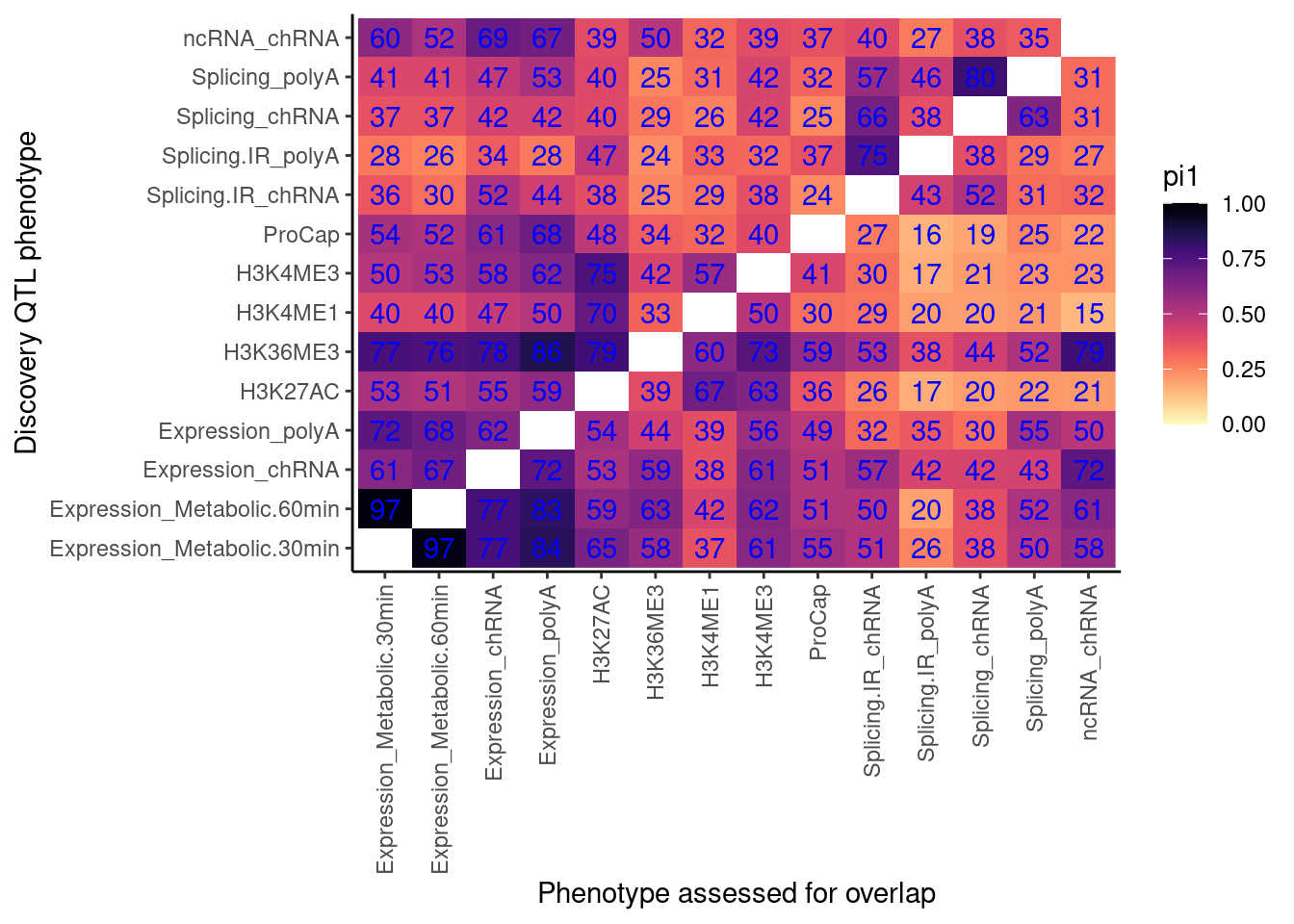

That looks better. Now let’s recode the activiting promoter marks to either distal promoter, host-gene promoter, or distal enhancer. First read in mapping of peaks to TSS

PeaksToTSS <- Sys.glob("../code/Misc/PeaksClosestToTSS/*_assigned.tsv.gz") %>%
  setNames(str_replace(., "../code/Misc/PeaksClosestToTSS/(.+?)_assigned.tsv.gz", "\\1")) %>%
  lapply(read_tsv) %>%
  bind_rows(.id="ChromatinMark") %>%
  mutate(GenePeakPair = paste(gene, peak, sep = ";")) %>%
  distinct(ChromatinMark, peak, gene, .keep_all=T)

GeneWindows <- dat$GeneLocus %>% unique()
TSSGenes <- PeaksToTSS$gene %>% unique()

length(GeneWindows)

[1] 13800

length(TSSGenes)

[1] 28091

intersect(GeneWindows, TSSGenes) %>% length()

[1] 12903

dat.split.added.union.activating.marks <- dat %>%
  filter(PC1 %in% RecodeIncludePCs) %>%
  filter(PC2 %in% RecodeIncludePCs) %>%
  mutate(PC1 = recode(PC1, !!!RecodeVec)) %>%
  mutate(PC2 = recode(PC2, !!!RecodeVec)) %>%
  mutate(PC1 = case_when(
    paste(GeneLocus, P1, sep=";") %in% PeaksToTSS$GenePeakPair ~ "ActivatingMark_HostGenePromoter",
    P1 %in% PeaksToTSS$peak ~ "ActivatingMark_OtherGenePromoter",
    PC1 %in% c("H3K4ME1", "H3K4ME3", "H3K27AC") ~ "ActivatingMark_Enhancer",
    TRUE ~ PC1
  )) %>%
  mutate(PC2 = case_when(
    paste(GeneLocus, P2, sep=";") %in% PeaksToTSS$GenePeakPair ~ "ActivatingMark_HostGenePromoter",
    P2 %in% PeaksToTSS$peak ~ "ActivatingMark_OtherGenePromoter",
    PC2 %in% c("H3K4ME1", "H3K4ME3", "H3K27AC") ~ "ActivatingMark_Enhancer",
    TRUE ~ PC2
  ))

dat.split.added.union.activating.marks <-
  bind_rows(dat.split.added.union.activating.marks, 
    (dat.split.added.union.activating.marks %>% filter(str_detect(PC1, "ActivatingMark")) %>%
    mutate(PC1 = case_when(
      str_detect(PC1, "ActivatingMark") ~ "AnyActivatingMark",
      TRUE ~ PC1
    ))),
    (dat.split.added.union.activating.marks %>% filter(str_detect(PC2, "ActivatingMark")) %>%
    mutate(PC2 = case_when(
      str_detect(PC2, "ActivatingMark") ~ "AnyActivatingMark",
      TRUE ~ PC2
    )))) %>%
  group_by(PC1, P1, PC2) %>%
  mutate(test.stat.obs = -log10(min(trait.x.p.in.y))) %>%
  ungroup() %>%
  add_count(PC1, P1, PC2) %>%
  filter(n<=250) %>%
  group_by(PC1, PC2) %>%
  rowwise() %>%
  mutate(Pvals.For.Pi1 = 1-ecdf.functions[[n]](test.stat.obs)) %>%
  ungroup() %>%
  select(PC1, PC2, Pvals.For.Pi1) %>%
  filter(!PC1==PC2) %>%
  split(paste(.$PC1, .$PC2, sep = ";"))


lapply(dat.split.added.union.activating.marks, CalculatePi1, pi0.method="bootstrap") %>%
  unlist() %>%
  data.frame(pi1=.) %>%
  rownames_to_column("PC1_PC2") %>%
  separate(PC1_PC2, into=c("PC1", "PC2"), sep=';') %>%
  # filter(!(PC1=="ActivatingMark" | PC2 == "ActivatingMark") ) %>%
  mutate(TextColor = case_when(
    pi1 >= 0.7 ~ "white",
    TRUE ~ "black"
  )) %>%
ggplot(aes(x=PC1, y=PC2, fill=pi1, color=TextColor)) +
  geom_raster() +
  geom_text(aes(label=signif(pi1*100, 2))) +
  scale_color_identity() +
  scale_fill_viridis(option="A", direction = -1, limits=c(0,1)) +
  coord_flip() +
  theme_classic() +
  theme(axis.text.x = element_text(angle = 90, vjust = 0.5, hjust=1)) +
  labs(x="Discovery QTL phenotype", y="Phenotype assessed for overlap")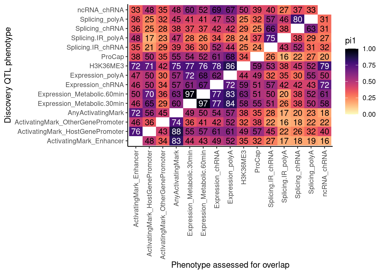

Some of these pi1 estimates don’t make sense. When discovery QTL is “ActivatingMark_*“, pi1 assessed in”AnyActivatingMark" should be 100%… Let’s check the histograms…

dat.split.added.union.activating.marks %>%
  bind_rows(.id="ID") %>%
  filter(PC2 == "AnyActivatingMark") %>%
  split(paste(.$PC1, .$PC2, sep = ";")) %>%
  lapply(CalculatePi1, lambda=0.5, pi0.method="bootstrap") %>%
  unlist() %>%
  data.frame(pi1=.)

                                                         pi1
ActivatingMark_Enhancer;AnyActivatingMark          0.8318326
ActivatingMark_HostGenePromoter;AnyActivatingMark  0.8733038
ActivatingMark_OtherGenePromoter;AnyActivatingMark 0.7430970
Expression_Metabolic.30min;AnyActivatingMark       0.5855742
Expression_Metabolic.60min;AnyActivatingMark       0.6085198
Expression_chRNA;AnyActivatingMark                 0.5549810
Expression_polyA;AnyActivatingMark                 0.5580077
H3K36ME3;AnyActivatingMark                         0.7095374
ProCap;AnyActivatingMark                           0.5314758
Splicing.IR_chRNA;AnyActivatingMark                0.3916971
Splicing.IR_polyA;AnyActivatingMark                0.4455069
Splicing_chRNA;AnyActivatingMark                   0.3747645
Splicing_polyA;AnyActivatingMark                   0.4190953
ncRNA_chRNA;AnyActivatingMark                      0.4601645

QvalueObj <- dat.split.added.union.activating.marks %>%
  bind_rows(.id="ID") %>%
  filter(PC1 == "ActivatingMark_Enhancer" & PC2 == "AnyActivatingMark") %>%
  pull(Pvals.For.Pi1) %>%
  pi0est(pi0.method="bootstrap")

plot(QvalueObj$lambda, QvalueObj$pi0.lambda)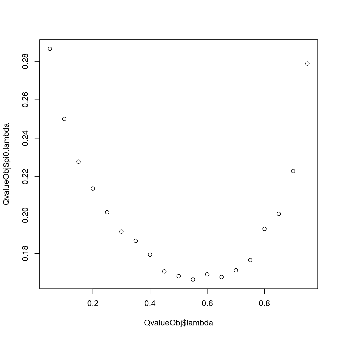

dat.split.added.union.activating.marks %>%
  bind_rows(.id="ID") %>%
  filter(str_detect(PC1, "ActivatingMark") & str_detect(PC2, "ActivatingMark")) %>%
  ggplot(aes(x=Pvals.For.Pi1)) +
  geom_histogram() +
  facet_wrap(~ID, scales = "free_y") +
  theme_bw()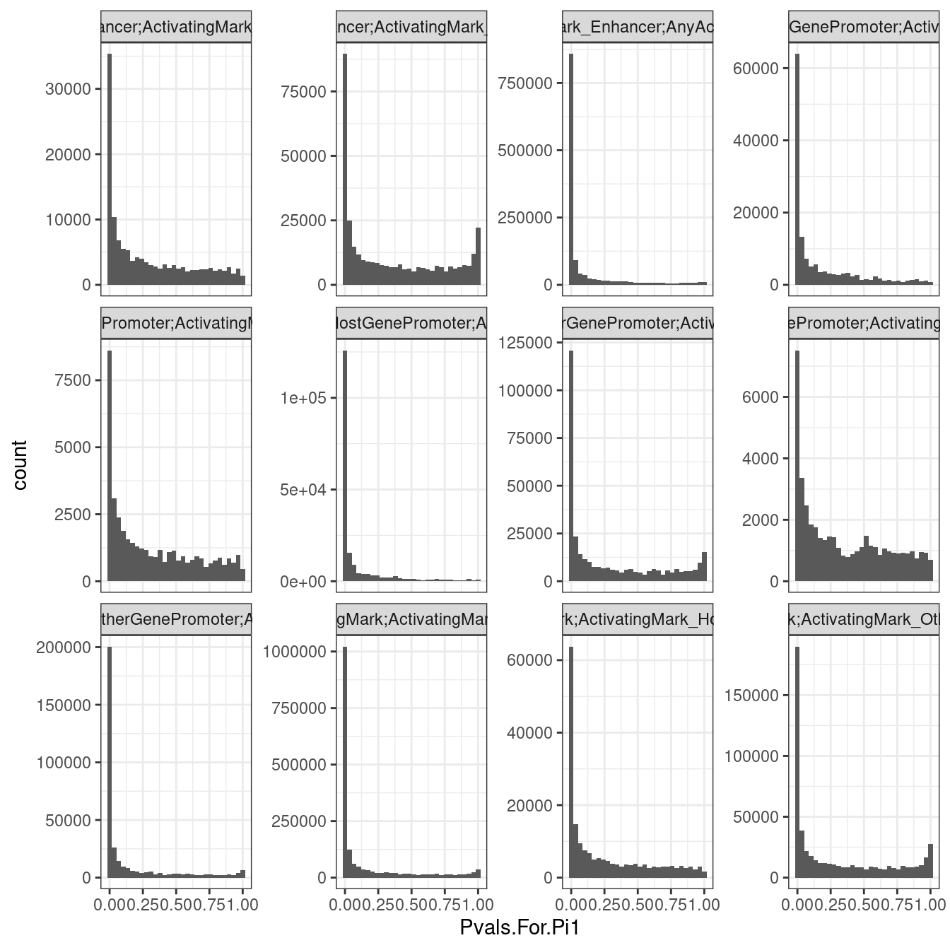

dat.split.added.union.activating.marks %>%
  bind_rows(.id="ID") %>%
  filter(PC1=="Expression_Metabolic.30min", str_detect(PC2, "ActivatingMark")) %>%
  ggplot(aes(x=Pvals.For.Pi1)) +
  geom_histogram() +
  facet_wrap(~ID, scales = "free_y") +
  theme_bw()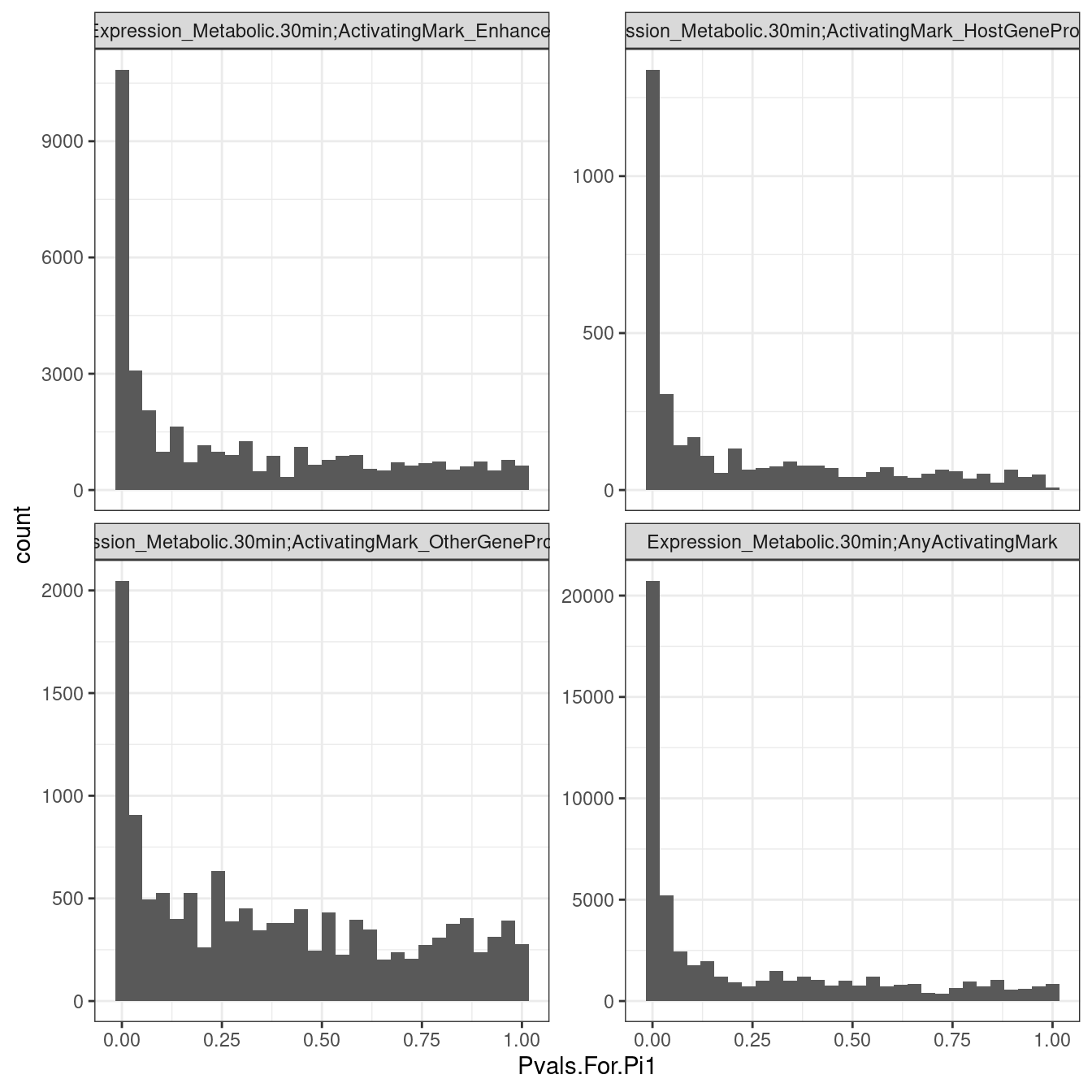

Hmm, I suspect this is another problem like I described before where there are many non-signifant non-independent tests that make the Pvalue distribution a tad conservative when there is a one-to-many phenotype mapping. I note that Metabolic.30min vs Metabolic.60min don’t seem to have this problem, as the pi1 staistic is near 100%, and it doesn’t have a the one-to-many mapping problem. Well I am not too concerned for now, I will just have to remember that when there are many ascertainment phenotypes that get tested against each discovery, that the pi1 estimates may be a bit convervatice (smaller than truth).

Ok now make the plot with different FDR thresholds:

# Make a function to re-use

CalculatePi1Matrix <- function(dat, DiscoveryFDR=0.1){
  dat.split.added.union.activating.marks <- dat %>%
    filter(FDR.x <= DiscoveryFDR) %>%
    filter(PC1 %in% RecodeIncludePCs) %>%
    filter(PC2 %in% RecodeIncludePCs) %>%
    mutate(PC1 = recode(PC1, !!!RecodeVec)) %>%
    mutate(PC2 = recode(PC2, !!!RecodeVec)) %>%
    mutate(PC1 = case_when(
      paste(GeneLocus, P1, sep=";") %in% PeaksToTSS$GenePeakPair ~ "ActivatingMark_HostGenePromoter",
      P1 %in% PeaksToTSS$peak ~ "ActivatingMark_OtherGenePromoter",
      PC1 %in% c("H3K4ME1", "H3K4ME3", "H3K27AC") ~ "ActivatingMark_Enhancer",
      TRUE ~ PC1
    )) %>%
    mutate(PC2 = case_when(
      paste(GeneLocus, P2, sep=";") %in% PeaksToTSS$GenePeakPair ~ "ActivatingMark_HostGenePromoter",
      P2 %in% PeaksToTSS$peak ~ "ActivatingMark_OtherGenePromoter",
      PC2 %in% c("H3K4ME1", "H3K4ME3", "H3K27AC") ~ "ActivatingMark_Enhancer",
      TRUE ~ PC2
    ))
  
  dat.split.added.union.activating.marks <-
    bind_rows(dat.split.added.union.activating.marks, 
      (dat.split.added.union.activating.marks %>% filter(str_detect(PC1, "ActivatingMark")) %>%
      mutate(PC1 = case_when(
        str_detect(PC1, "ActivatingMark") ~ "AnyActivatingMark",
        TRUE ~ PC1
      ))),
      (dat.split.added.union.activating.marks %>% filter(str_detect(PC2, "ActivatingMark")) %>%
      mutate(PC2 = case_when(
        str_detect(PC2, "ActivatingMark") ~ "AnyActivatingMark",
        TRUE ~ PC2
      )))) %>%
    group_by(PC1, P1, PC2) %>%
    mutate(test.stat.obs = -log10(min(trait.x.p.in.y))) %>%
    ungroup() %>%
    add_count(PC1, P1, PC2) %>%
    filter(n<=250) %>%
    group_by(PC1, PC2) %>%
    rowwise() %>%
    mutate(Pvals.For.Pi1 = 1-ecdf.functions[[n]](test.stat.obs)) %>%
    ungroup() %>%
    select(PC1, PC2, Pvals.For.Pi1) %>%
    filter(!PC1==PC2) %>%
    split(paste(.$PC1, .$PC2, sep = ";"))
  
  dat.pi1 <- lapply(dat.split.added.union.activating.marks, CalculatePi1, pi0.method="bootstrap") %>%
    unlist() %>%
    data.frame(pi1=.) %>%
    rownames_to_column("PC1_PC2") %>%
    separate(PC1_PC2, into=c("PC1", "PC2"), sep=';') %>%
    mutate(DiscoveryFDR = DiscoveryFDR) %>%
    mutate(TextColor = case_when(
      pi1 >= 0.7 ~ "white",
      TRUE ~ "black"
    ))
return(dat.pi1)
}

dat.pi.AtThresholds <- bind_rows(
  CalculatePi1Matrix(dat, DiscoveryFDR=0.1),
  CalculatePi1Matrix(dat, DiscoveryFDR=0.05),
  CalculatePi1Matrix(dat, DiscoveryFDR=0.01)
)

pi.heatmap <- ggplot(dat.pi.AtThresholds, aes(x=PC1, y=PC2, fill=pi1, color=TextColor)) +
  geom_raster() +
  geom_text(aes(label=signif(pi1*100, 2))) +
  scale_fill_viridis(option="A", direction = -1, limits=c(0,1)) +
  scale_color_identity() +
  facet_wrap(~DiscoveryFDR) +
  coord_flip() +
  theme_classic() +
  theme(axis.text.x = element_text(angle = 90, vjust = 0.5, hjust=1)) +
  labs(x="Discovery QTL phenotype", y="Phenotype assessed for overlap", "Pi1 of xQTL among Discovery QTL classes")
pi.heatmap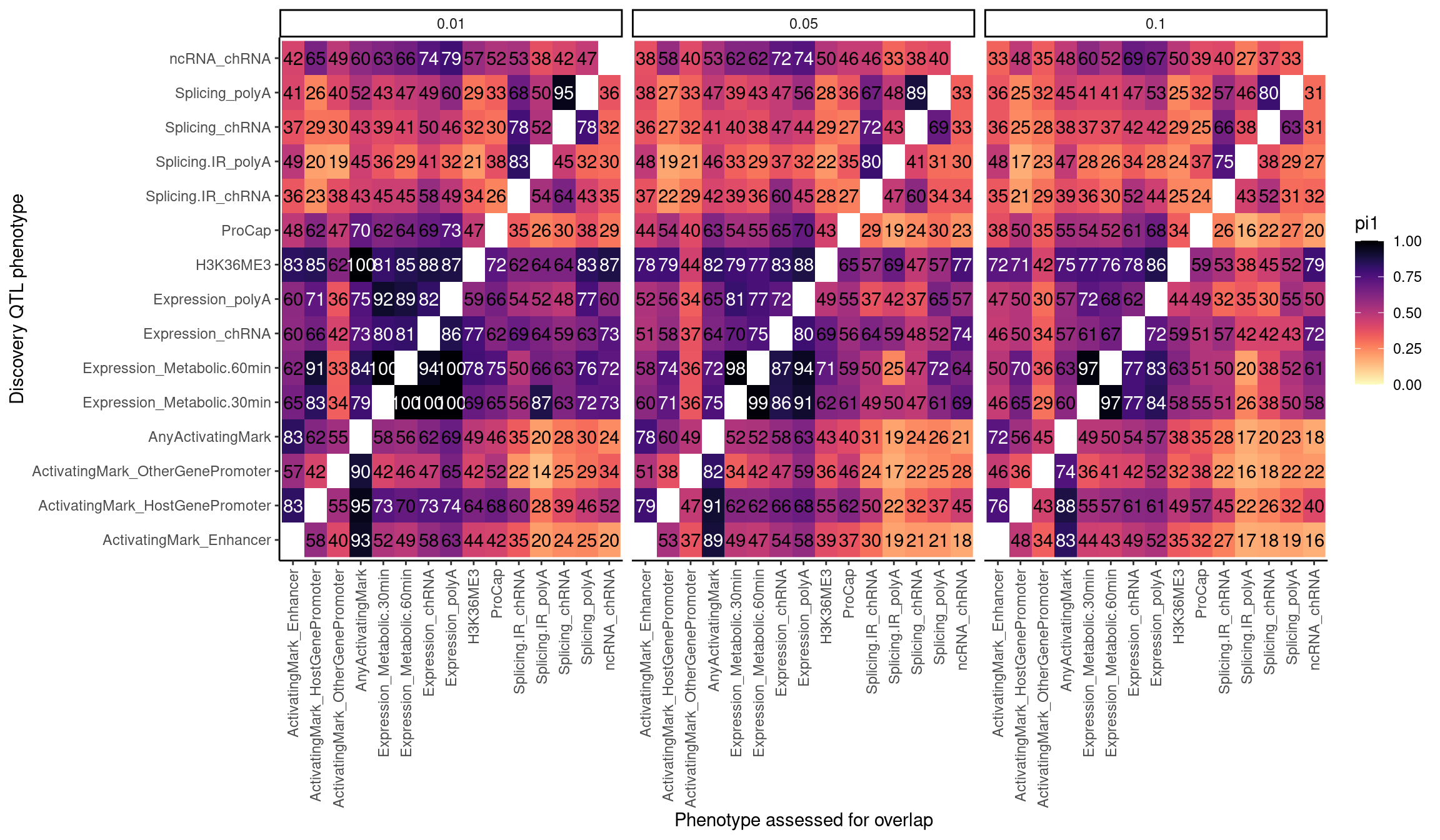

Consistent with the one-to-many explanation of pi1 being overly conservatice, when there are less phenotypes to map to one (ie when the 0.01 facet), the ActinvatingMark_* to AnyActivatingMark approaches 100%.

dat %>% pull(PC1) %>% unique()

 [1] "chRNA.Expression_cheRNA"             "chRNA.Expression_eRNA"              
 [3] "chRNA.Expression_lncRNA"             "chRNA.Expression_snoRNA"            
 [5] "chRNA.Expression.Splicing"           "chRNA.IER"                          
 [7] "chRNA.IRjunctions"                   "chRNA.IR"                           
 [9] "chRNA.Slopes"                        "chRNA.Splicing"                     
[11] "CTCF"                                "Expression.Splicing"                
[13] "Expression.Splicing.Subset_YRI"      "H3K27AC"                            
[15] "H3K36ME3"                            "H3K4ME1"                            
[17] "H3K4ME3"                             "MetabolicLabelled.30min.IER"        
[19] "MetabolicLabelled.30min.IRjunctions" "MetabolicLabelled.30min.IR"         
[21] "MetabolicLabelled.30min"             "MetabolicLabelled.30min.Splicing"   
[23] "MetabolicLabelled.60min.IER"         "MetabolicLabelled.60min.IRjunctions"
[25] "MetabolicLabelled.60min.IR"          "MetabolicLabelled.60min"            
[27] "MetabolicLabelled.60min.Splicing"    "polyA.IER"                          
[29] "polyA.IRjunctions"                   "polyA.IR"                           
[31] "polyA.IR.Subset_YRI"                 "polyA.Splicing"                     
[33] "polyA.Splicing.Subset_YRI"           "ProCap"                             

sessionInfo()

R version 3.6.1 (2019-07-05)
Platform: x86_64-pc-linux-gnu (64-bit)
Running under: CentOS Linux 7 (Core)

Matrix products: default
BLAS/LAPACK: /software/openblas-0.2.19-el7-x86_64/lib/libopenblas_haswellp-r0.2.19.so

locale:
 [1] LC_CTYPE=en_US.UTF-8 LC_NUMERIC=C         LC_TIME=C           
 [4] LC_COLLATE=C         LC_MONETARY=C        LC_MESSAGES=C       
 [7] LC_PAPER=C           LC_NAME=C            LC_ADDRESS=C        
[10] LC_TELEPHONE=C       LC_MEASUREMENT=C     LC_IDENTIFICATION=C 

attached base packages:
[1] stats     graphics  grDevices utils     datasets  methods   base     

other attached packages:
 [1] pROC_1.15.0       GGally_1.4.0      qvalue_2.16.0     data.table_1.14.2
 [5] gplots_3.0.1.1    viridis_0.5.1     viridisLite_0.3.0 forcats_0.4.0    
 [9] stringr_1.4.0     dplyr_1.0.9       purrr_0.3.4       readr_1.3.1      
[13] tidyr_1.2.0       tibble_3.1.7      ggplot2_3.3.6     tidyverse_1.3.0  

loaded via a namespace (and not attached):
 [1] httr_1.4.4         jsonlite_1.6       splines_3.6.1      R.utils_2.9.0     
 [5] modelr_0.1.8       gtools_3.9.2.2     assertthat_0.2.1   highr_0.9         
 [9] cellranger_1.1.0   yaml_2.2.0         pillar_1.7.0       backports_1.4.1   
[13] glue_1.6.2         digest_0.6.20      RColorBrewer_1.1-2 promises_1.0.1    
[17] rvest_0.3.5        colorspace_1.4-1   R.oo_1.22.0        htmltools_0.5.3   
[21] httpuv_1.5.1       plyr_1.8.4         pkgconfig_2.0.2    broom_1.0.0       
[25] haven_2.3.1        scales_1.1.0       gdata_2.18.0       later_0.8.0       
[29] git2r_0.26.1       farver_2.1.0       generics_0.1.3     ellipsis_0.3.2    
[33] withr_2.5.0        cli_3.3.0          magrittr_1.5       crayon_1.3.4      
[37] readxl_1.3.1       evaluate_0.15      R.methodsS3_1.7.1  fs_1.5.2          
[41] fansi_0.4.0        xml2_1.3.2         tools_3.6.1        hms_0.5.3         
[45] lifecycle_1.0.1    munsell_0.5.0      reprex_0.3.0       compiler_3.6.1    
[49] caTools_1.17.1.2   rlang_1.0.5        grid_3.6.1         rstudioapi_0.14   
[53] labeling_0.3       bitops_1.0-6       rmarkdown_1.13     gtable_0.3.0      
[57] DBI_1.1.0          reshape_0.8.8      reshape2_1.4.3     R6_2.4.0          
[61] gridExtra_2.3      lubridate_1.7.4    knitr_1.39         fastmap_1.1.0     
[65] utf8_1.1.4         workflowr_1.6.2    rprojroot_2.0.2    KernSmooth_2.23-15
[69] stringi_1.4.3      Rcpp_1.0.5         vctrs_0.4.1        dbplyr_1.4.2      
[73] tidyselect_1.1.2   xfun_0.31