20191001_GtexAnnotations
Ben Fair
10/1/2019
Last updated: 2019-10-03
Checks: 6 1
Knit directory: Comparative_eQTL/analysis/
This reproducible R Markdown analysis was created with workflowr (version 1.4.0). The Checks tab describes the reproducibility checks that were applied when the results were created. The Past versions tab lists the development history.
The R Markdown is untracked by Git. To know which version of the R Markdown file created these results, you’ll want to first commit it to the Git repo. If you’re still working on the analysis, you can ignore this warning. When you’re finished, you can run wflow_publish to commit the R Markdown file and build the HTML.
Great job! The global environment was empty. Objects defined in the global environment can affect the analysis in your R Markdown file in unknown ways. For reproduciblity it’s best to always run the code in an empty environment.
The command set.seed(20190319) was run prior to running the code in the R Markdown file. Setting a seed ensures that any results that rely on randomness, e.g. subsampling or permutations, are reproducible.
Great job! Recording the operating system, R version, and package versions is critical for reproducibility.
Nice! There were no cached chunks for this analysis, so you can be confident that you successfully produced the results during this run.
Great job! Using relative paths to the files within your workflowr project makes it easier to run your code on other machines.
Great! You are using Git for version control. Tracking code development and connecting the code version to the results is critical for reproducibility. The version displayed above was the version of the Git repository at the time these results were generated.
Note that you need to be careful to ensure that all relevant files for the analysis have been committed to Git prior to generating the results (you can use wflow_publish or wflow_git_commit). workflowr only checks the R Markdown file, but you know if there are other scripts or data files that it depends on. Below is the status of the Git repository when the results were generated:
Ignored files:
    Ignored:    .DS_Store
    Ignored:    .Rhistory
    Ignored:    .Rproj.user/
    Ignored:    analysis/.DS_Store
    Ignored:    analysis/20190521_eQTL_CrossSpeciesEnrichment_cache/
    Ignored:    analysis_temp/.DS_Store
    Ignored:    code/.DS_Store
    Ignored:    code/snakemake_workflow/.DS_Store
    Ignored:    data/.DS_Store
    Ignored:    data/PastAnalysesDataToKeep/.DS_Store
    Ignored:    docs/.DS_Store
    Ignored:    docs/assets/.DS_Store

Untracked files:
    Untracked:  analysis/20191001_GtexAnnotations.Rmd
    Untracked:  analysis_temp/20190716_VarianceInsteadOfEgenes_2.Rmd
    Untracked:  docs/figure/20190930_OverdispersionEstimates.Rmd/

Unstaged changes:
    Deleted:    analysis/20190716_VarianceInsteadOfEgenes_2.Rmd
    Modified:   analysis/20190930_OverdispersionEstimates.Rmd
Note that any generated files, e.g. HTML, png, CSS, etc., are not included in this status report because it is ok for generated content to have uncommitted changes.
There are no past versions. Publish this analysis with wflow_publish() to start tracking its development.
From my dataset of gene expression measurements across 39 chimp individuals (RNA-seq from heart tissue) and ~39 human individuals (~50 RNA-seq sampels randomly chosen from human GTEx datasets, then culled to exclude outliers and lowly sequenced samples) I am interested in quantifying gene expression dispersion within each population. I had previously made the observation that gene expression overdispersion is well correlated (\(R^2\approx0.5\)) between the two species, even after regressing out the fact that variance is correlated to expression (due to both biological and statstical reasons). This amount of correlation is higher than I would have guessed, given how small the overlap is between eGenes that I could detect. However, I still don’t have a sense of what I should have expected. To gain some intuition on this, I would like to use other GTEx tissues to estimate gene-wise overdispersion parameters, and compare the correlation across tissues. First, let’s peruse the GTEx samples available to us, to pick ~40 reasonable samples per tissue for this analysis.
library(tidyverse)

Samples <- read.table("../data/GTExAnnotations/GTEx_Analysis_v8_Annotations_SampleAttributesDS.txt", header=T, sep='\t', quote="")
Subjects <- read.table("../data/GTExAnnotations/GTEx_Analysis_v8_Annotations_SubjectPhenotypesDS.txt", header=T, sep='\t')
GtexColors <- read.table("../data/GTEx_Analysis_TissueColorCodes.txt", sep='\t', header=T, stringsAsFactors = F) %>% mutate(HEX=paste0("#",Color.code))

TissueColorVector <- GtexColors$HEX
names(TissueColorVector)<-GtexColors$Tissue

#Num samples per tissue. Note that I may want to filter out some samples to draw from ones where experimental protocols (like RNA extraction method) were kept reasonably constant
Samples %>%
  filter(SMAFRZE=="RNASEQ") %>%
  count(SMTSD,SMNABTCHT) %>%
  filter(SMTSD %in% GtexColors$Tissue) %>% mutate(sum=sum(n)) %>%
  ggplot(aes(x=SMTSD, y=n, fill=SMTSD, color=SMNABTCHT)) +
    geom_col(show.legend = T) +
    ylab("Number Samples") +
    theme_bw() +
    scale_fill_manual(values=TissueColorVector, guide=FALSE) +
    theme(axis.text.x = element_text(angle = 90, hjust = 1, vjust=0.5)) +
    theme(legend.position="top") +
    guides(color=guide_legend(nrow=2,byrow=TRUE))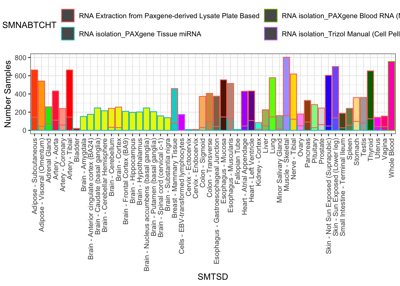
#Histogram of mapping rate
hist(Samples$SMMAPRT)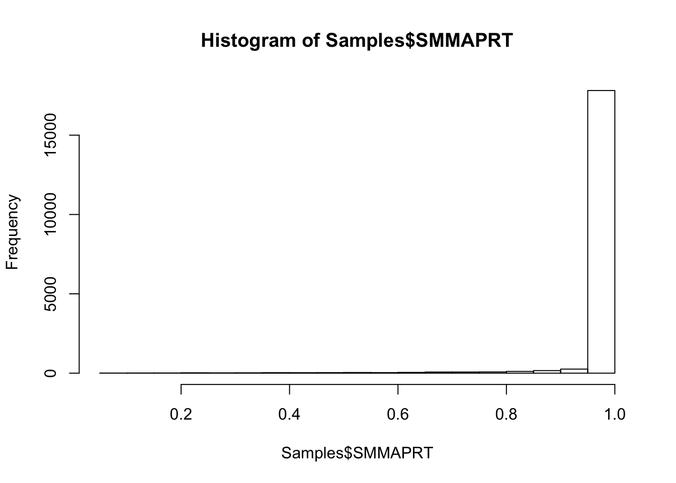
#Histogram of rRNA mapping rate
hist(Samples$SMRRNART)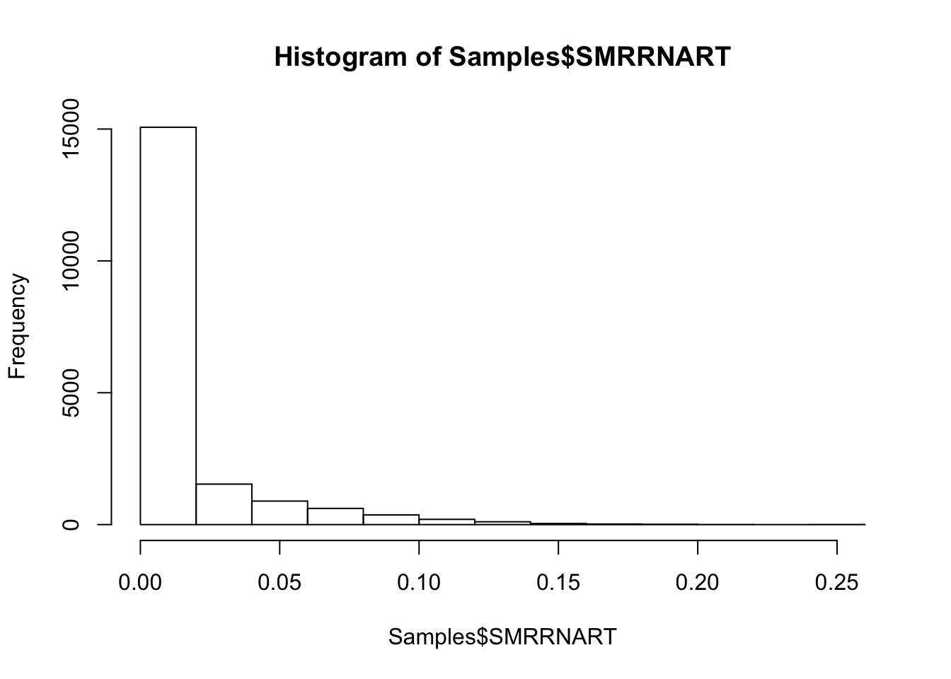
#Histogram of exonic mapping rate
hist(Samples$SMEXNCRT)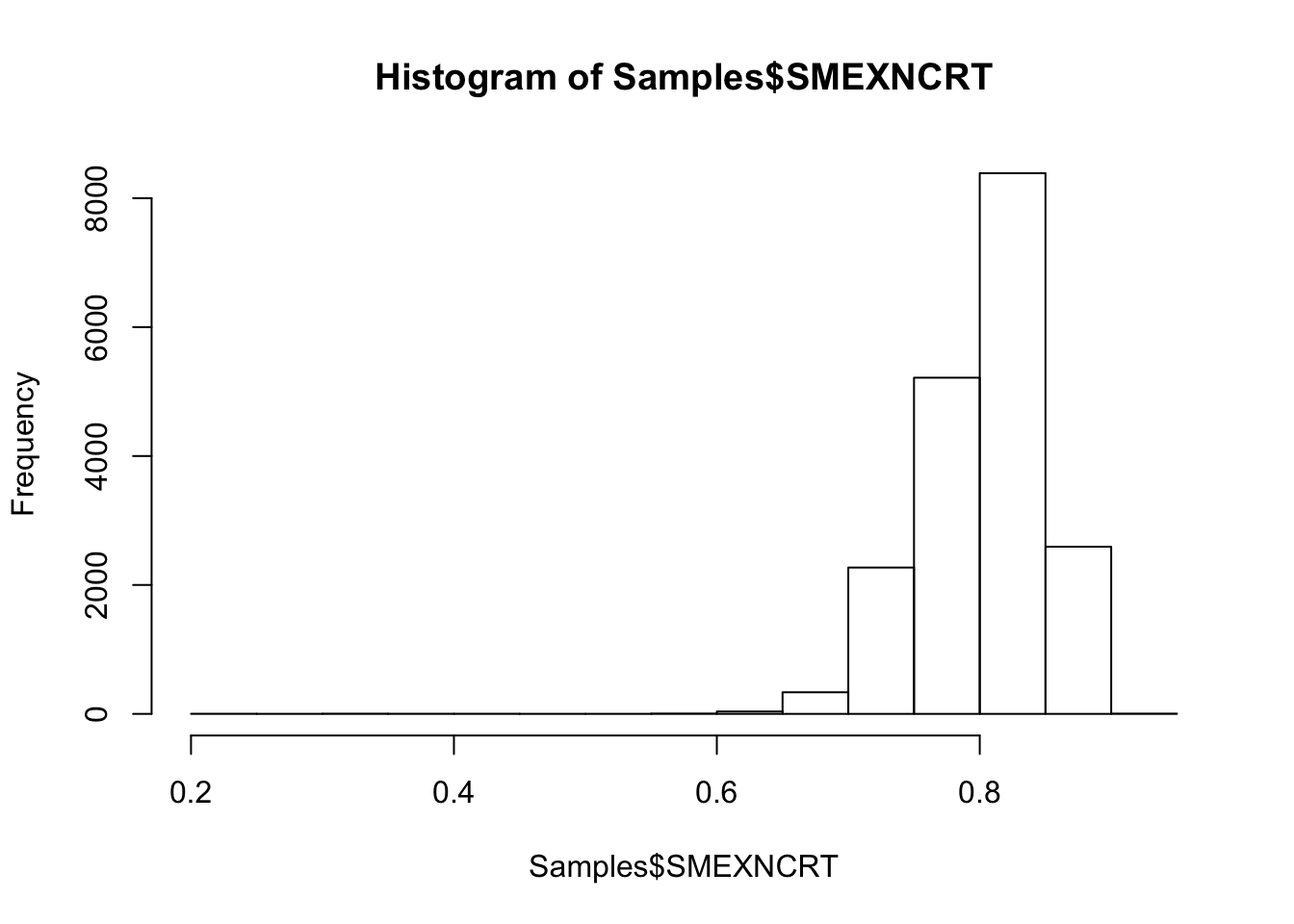
#Histogram of mapped library size
hist(log10(Samples$SMMPPD))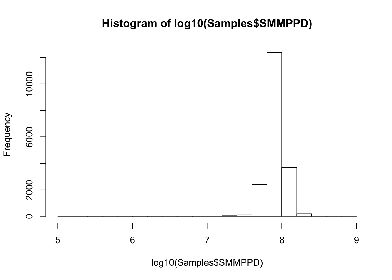
#RIN score
hist(Samples$SMRIN)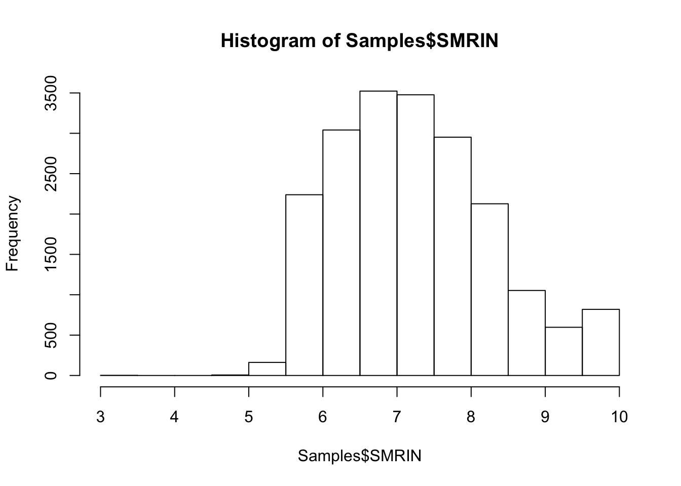
#types of library preps
table(Samples$SMGEBTCHT)
                Affymetrix Expression
                                  837
                             ChIP-Seq
                                  356
                            DroNc-seq
                                   20
   Exome Express (Agilent SureSelect)
                                  100
       Illumina Human Exome SNP Array
                                  189
              Illumina OMNI SNP Array
                                  462
PCR-Free 30x Coverage WGS v1 (HiSeqX)
                                  249
    PCR+ 30x Coverage WGS (HiSeq2000)
                                   79
 PCR+ 30x Coverage WGS v1 (HiSeq2000)
                                    1
    PCR+ 30x Coverage WGS v1 (HiSeqX)
                                    1
    PCR+ 30x Coverage WGS v2 (HiSeqX)
                                  579
                              RIP-Seq
                                  226
   Standard Exome Sequencing v2 (ICE)
                                   80
   Standard Exome Sequencing v3 (ICE)
                                  510
   Standard Exome Sequencing v5 (ICE)
                                  315
                             Tech Dev
                                   24
      Tech Dev - Large Insert RNA-seq
                                   65
                            TruSeq.v1
                                18858
#types of nucleic acid preps
table(Samples$SMNABTCHT)
                                                   376
DNA Extraction from Paxgene-derived Lysate Plate Based
                                                   117
      DNA Isolation from Tissue via QIAgen Spin Column
                                                    87
      DNA Isolation of Compromised Blood with Autopure
                                                    30
  DNA isolation_Whole Blood_QIAGEN Puregene (Autopure)
                                                    40
    DNA isolation_Whole Blood_QIAGEN Puregene (Manual)
                                                  2285
RNA Extraction from Paxgene-derived Lysate Plate Based
                                                 11760
              RNA isolation_PAXgene Blood RNA (Manual)
                                                   933
                    RNA isolation_PAXgene Tissue miRNA
                                                  6387
             RNA isolation_Trizol Manual (Cell Pellet)
                                                   936
#sample type. RNASEQ type was deemed suitable for GTEx v8 eQTL calling
table(Samples$SMAFRZE)
        EXCLUDE    OMNI  RNASEQ     WES     WGS
    602    2700     450   17382     979     838
#Now let's randomly pick ~40 samples that are TruSeq.v1 and have coverage comparable to my ChimpSamples (~70M mapped reads), and are similar in other metrics (RNA Extraction from Paxgene-derived Lysate Plate Based).
Mode <- function(x) {
ux <- unique(x)
ux[which.max(tabulate(match(x, ux)))]
}
# Apply filters, like keeping RNA-extraction method consistent within tissue, minimum mapping rate, etc.
SamplesFilteredForTissuesSuitableForAnalysis <- Samples %>%
mutate(IndidualID=gsub("GTEX-(\\w+)-.+", "\\1", SAMPID, perl=T)) %>%
# filter(SMNABTCHT %in% c("RNA Extraction from Paxgene-derived Lysate Plate Based")) %>%
filter(SMAFRZE=="RNASEQ") %>%
group_by(SMTSD) %>%
mutate(c=Mode(SMNABTCHT)) %>%
filter(quantile(SMMPPD, 0.1)<SMMPPD &
quantile(SMMAPRT, 0.1)<SMMAPRT &
quantile(SMRIN, 0.1)<SMRIN) %>%
ungroup() %>%
filter(SMNABTCHT==c) %>%
add_count(SMTSD, name="CountBeforeSampling") %>%
filter(SMTSD %in% GtexColors$Tissue) %>%
filter(CountBeforeSampling>40)
# Acceptable samples to draw from.
SamplesFilteredForTissuesSuitableForAnalysis %>%
group_by(SMTSD) %>%
count(SMTSD, SMNABTCHT) %>%
ggplot(aes(x=SMTSD, y=n, fill=SMTSD, color=SMNABTCHT)) +
geom_col(show.legend = T) +
ylab("Number Samples") +
theme_bw() +
scale_fill_manual(values=TissueColorVector, guide=FALSE) +
theme(axis.text.x = element_text(angle = 90, hjust = 1, vjust=0.5)) +
theme(legend.position="top") +
guides(color=guide_legend(nrow=2,byrow=TRUE))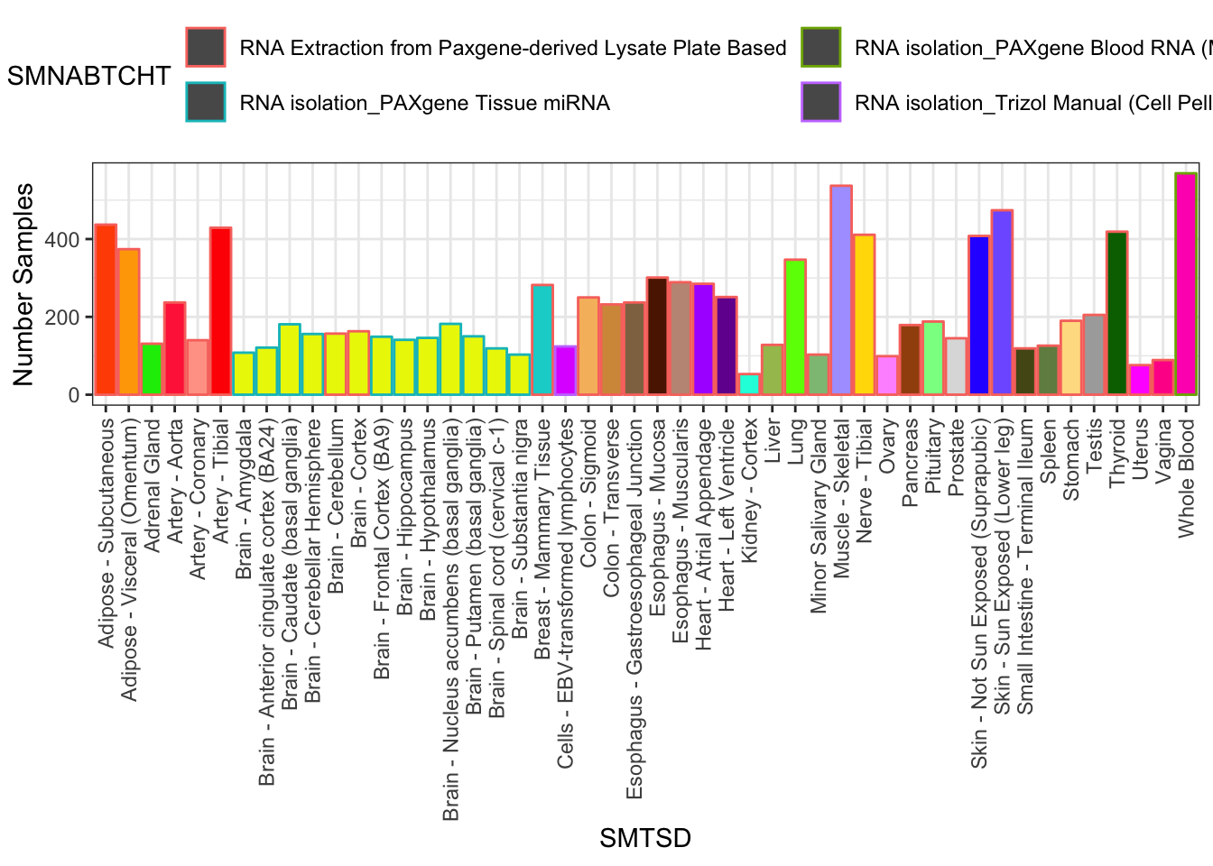
# Samples drawn at random to keep sample size consistent
set.seed(0)
SuitableSubsample <- SamplesFilteredForTissuesSuitableForAnalysis  %>%
  group_by(SMTSD) %>%
  sample_n(40) %>% ungroup()
SuitableSubsample %>%
  count(SMTSD, SMNABTCHT) %>%
  ggplot(aes(x=SMTSD, y=n, fill=SMTSD, color=SMNABTCHT)) +
    geom_col(show.legend = T) +
    ylab("Number Samples") +
    theme_bw() +
    scale_fill_manual(values=TissueColorVector, guide=FALSE) +
    theme(axis.text.x = element_text(angle = 90, hjust = 1, vjust=0.5)) +
    theme(legend.position="top") +
    guides(color=guide_legend(nrow=2,byrow=TRUE))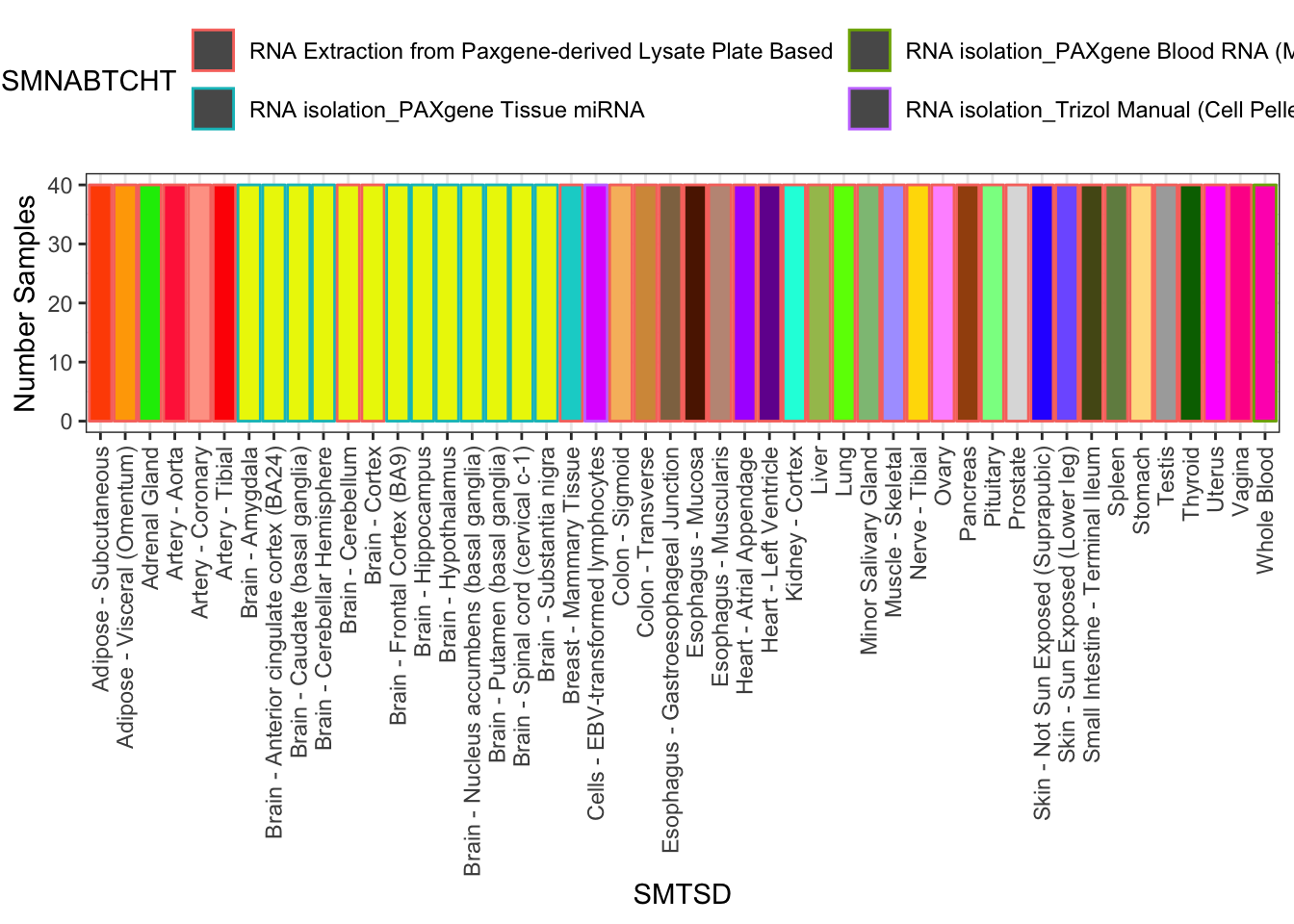
#How many tissues exist for this analysis
SuitableSubsample %>% distinct(SMTSD) %>% dim()
[1] 48 1# How many times do the same individuals show up in multiple tissues for this subsample?
SuitableSubsample %>% select(SAMPID, SMTSD, IndidualID) %>%
count(IndidualID) %>% pull(n) %>% hist(ylab="#individuals with X tissues in subsample")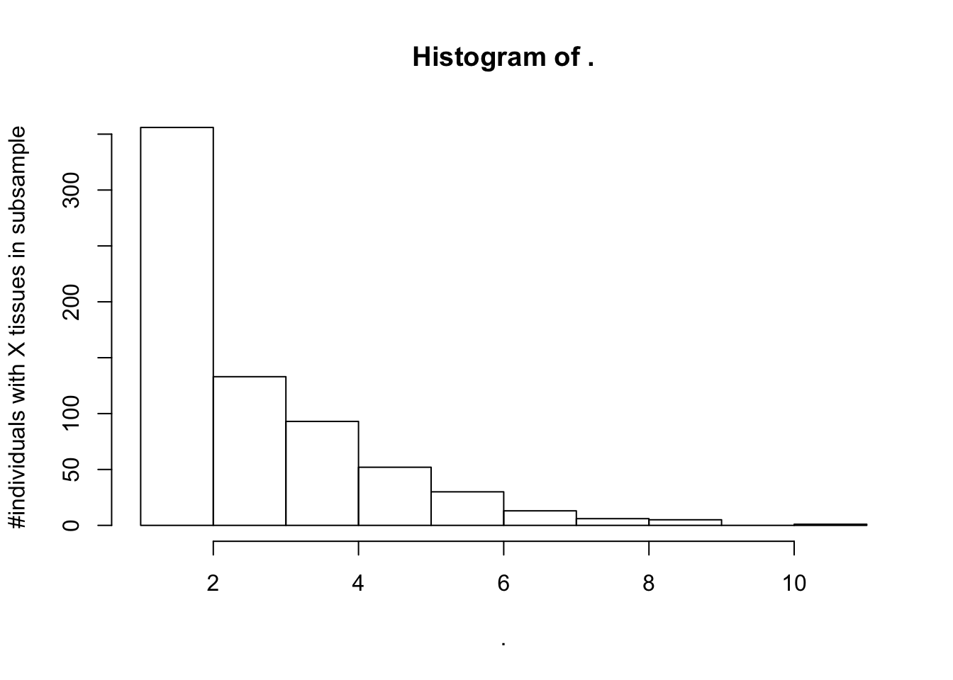
#Could be worth also making a subsample of the same 40 people for all tissues.
#Unfortunately that wouldn't be possible. Would need to consider less tissues, or less individuals.
SamplesFilteredForTissuesSuitableForAnalysis %>%
  count(IndidualID) %>% pull(n) %>% hist(ylab="#individuals with X tissues in subsample")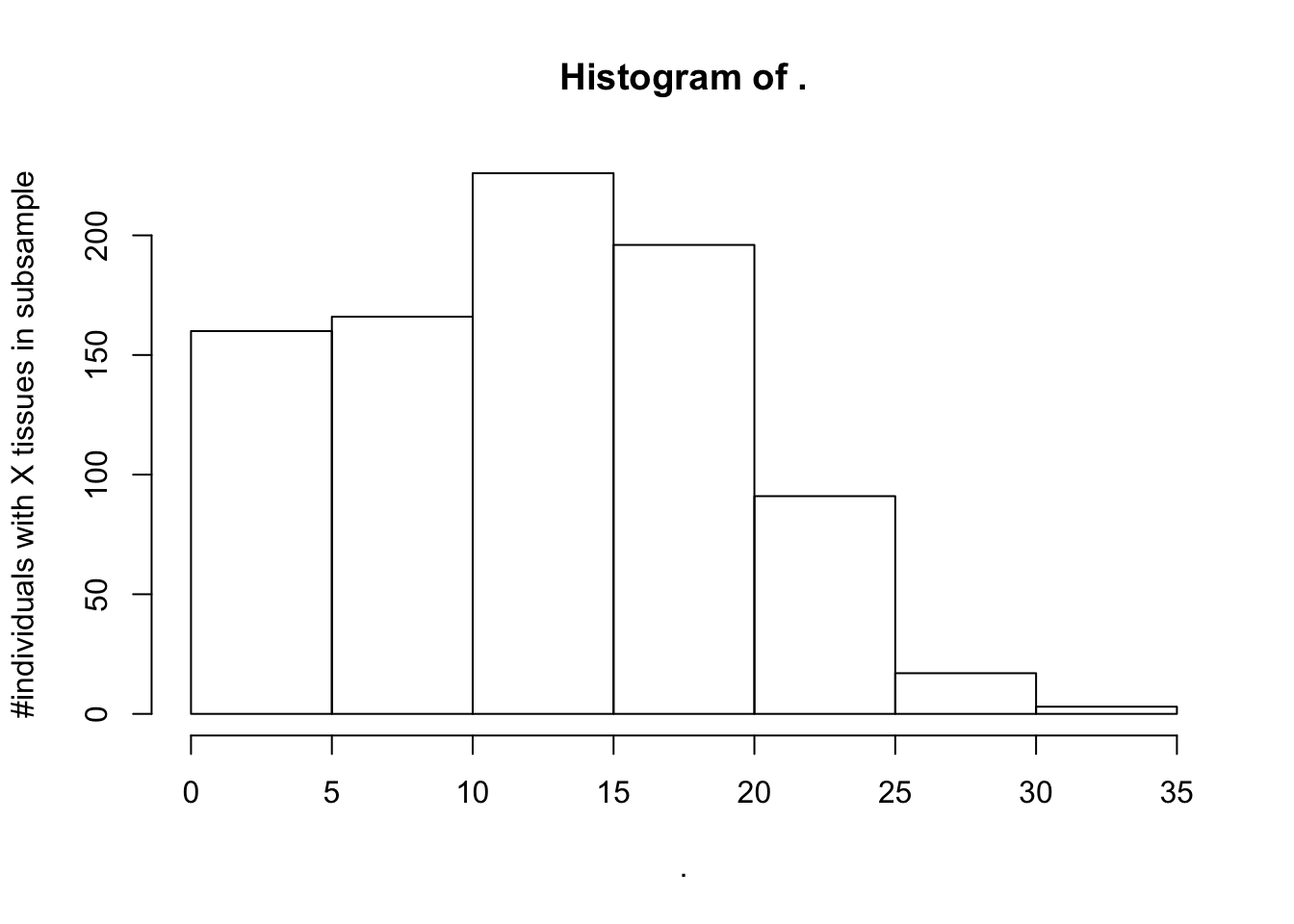
SuitableSubsample %>% select(SAMPID, SMTSD, IndidualID) %>%
  write.table("../data/OverdispersionGTExAnalysisSampleList.txt", sep="\t", quote=F, row.names = F)
sessionInfo()R version 3.5.1 (2018-07-02)
Platform: x86_64-apple-darwin15.6.0 (64-bit)
Running under: macOS 10.14
Matrix products: default
BLAS: /Library/Frameworks/R.framework/Versions/3.5/Resources/lib/libRblas.0.dylib
LAPACK: /Library/Frameworks/R.framework/Versions/3.5/Resources/lib/libRlapack.dylib
locale:
[1] en_US.UTF-8/en_US.UTF-8/en_US.UTF-8/C/en_US.UTF-8/en_US.UTF-8
attached base packages:
[1] stats graphics grDevices utils datasets methods base
other attached packages:
[1] forcats_0.4.0 stringr_1.4.0 dplyr_0.8.1 purrr_0.3.2
[5] readr_1.3.1 tidyr_0.8.3 tibble_2.1.3 ggplot2_3.1.1
[9] tidyverse_1.2.1
loaded via a namespace (and not attached):
[1] Rcpp_1.0.1 cellranger_1.1.0 plyr_1.8.4 pillar_1.4.1
[5] compiler_3.5.1 git2r_0.25.2 workflowr_1.4.0 tools_3.5.1
[9] digest_0.6.19 lubridate_1.7.4 jsonlite_1.6 evaluate_0.14
[13] nlme_3.1-140 gtable_0.3.0 lattice_0.20-38 pkgconfig_2.0.2
[17] rlang_0.3.4 cli_1.1.0 rstudioapi_0.10 yaml_2.2.0
[21] haven_2.1.0 xfun_0.7 withr_2.1.2 xml2_1.2.0
[25] httr_1.4.0 knitr_1.23 hms_0.4.2 generics_0.0.2
[29] fs_1.3.1 rprojroot_1.3-2 grid_3.5.1 tidyselect_0.2.5
[33] glue_1.3.1 R6_2.4.0 readxl_1.3.1 rmarkdown_1.13
[37] modelr_0.1.4 magrittr_1.5 backports_1.1.4 scales_1.0.0
[41] htmltools_0.3.6 rvest_0.3.4 assertthat_0.2.1 colorspace_1.4-1
[45] labeling_0.3 stringi_1.4.3 lazyeval_0.2.2 munsell_0.5.0
[49] broom_0.5.2 crayon_1.3.4