20190606_eGene_conservation
Ben Fair
6/6/2019
Last updated: 2019-08-06
Checks: 7 0
Knit directory: Comparative_eQTL/analysis/
This reproducible R Markdown analysis was created with workflowr (version 1.4.0). The Checks tab describes the reproducibility checks that were applied when the results were created. The Past versions tab lists the development history.
Great! Since the R Markdown file has been committed to the Git repository, you know the exact version of the code that produced these results.
Great job! The global environment was empty. Objects defined in the global environment can affect the analysis in your R Markdown file in unknown ways. For reproduciblity it’s best to always run the code in an empty environment.
The command set.seed(20190319) was run prior to running the code in the R Markdown file. Setting a seed ensures that any results that rely on randomness, e.g. subsampling or permutations, are reproducible.
Great job! Recording the operating system, R version, and package versions is critical for reproducibility.
Nice! There were no cached chunks for this analysis, so you can be confident that you successfully produced the results during this run.
Great job! Using relative paths to the files within your workflowr project makes it easier to run your code on other machines.
Great! You are using Git for version control. Tracking code development and connecting the code version to the results is critical for reproducibility. The version displayed above was the version of the Git repository at the time these results were generated.
Note that you need to be careful to ensure that all relevant files for the analysis have been committed to Git prior to generating the results (you can use wflow_publish or wflow_git_commit). workflowr only checks the R Markdown file, but you know if there are other scripts or data files that it depends on. Below is the status of the Git repository when the results were generated:
Ignored files:
    Ignored:    .DS_Store
    Ignored:    .Rhistory
    Ignored:    .Rproj.user/
    Ignored:    analysis/.DS_Store
    Ignored:    analysis/20190521_eQTL_CrossSpeciesEnrichment_cache/
    Ignored:    analysis_temp/.DS_Store
    Ignored:    code/.DS_Store
    Ignored:    code/snakemake_workflow/.DS_Store
    Ignored:    code/snakemake_workflow/rules/.eQTL_analysis.smk.swp
    Ignored:    data/.DS_Store
    Ignored:    data/PastAnalysesDataToKeep/.DS_Store
    Ignored:    docs/.DS_Store
    Ignored:    docs/assets/.DS_Store

Unstaged changes:
    Modified:   analysis/20190521_eQTL_CrossSpeciesEnrichment.Rmd
    Modified:   analysis/20190627_DiffContactsEgenes.Rmd
    Modified:   analysis/20190708_DiffContactsEgenes_CisWindowControlled.Rmd
    Modified:   analysis/20190716_VarianceInsteadOfEgenes.Rmd
    Modified:   analysis/index.Rmd
    Modified:   code/snakemake_workflow/Session.vim
    Modified:   code/snakemake_workflow/rules/eQTL_analysis.smk
Note that any generated files, e.g. HTML, png, CSS, etc., are not included in this status report because it is ok for generated content to have uncommitted changes.
These are the previous versions of the R Markdown and HTML files. If you’ve configured a remote Git repository (see ?wflow_git_remote), click on the hyperlinks in the table below to view them.
| File | Version | Author | Date | Message |
|---|---|---|---|---|
| Rmd | f469d6a | Benjmain Fair | 2019-07-16 | new analyses |
| Rmd | 22eda3a | Benjmain Fair | 2019-06-12 | update site |
| html | 22eda3a | Benjmain Fair | 2019-06-12 | update site |
library(plyr)
library(tidyverse)
library(knitr)
library(data.table)
library(ggpmisc)
library("clusterProfiler")
library("org.Hs.eg.db")
library(gridExtra)
# library(ggpubr)
Here the dataset is eQTLs called from a model with the following pre-testing filters/transformations/checks:
- cis-window=250kB
- MAF>10%
- genes tested must have >6 reads in 80% of samples
- lmm with genetic relatedness matrix produced by gemma
- Gene expression is standardized and normalized
- 10PCs added as covariates
- FDR estimated by Storey’s qvalue
- Pvalues well calibrated under a permutated null
First, Read in the data…
eQTLs <- read.table(gzfile("../data/PastAnalysesDataToKeep/20190521_eQTLs_250kB_10MAF.txt.gz"), header=T)
kable(head(eQTLs))| snps | gene | beta | statistic | pvalue | FDR | qvalue |
|---|---|---|---|---|---|---|
| ID.1.126459696.ACCCTAGTAAG.A | ENSPTRG00000001061 | 3.570039 | 12.50828 | 0 | 3.5e-06 | 3.5e-06 |
| ID.1.126465687.TTGT.A | ENSPTRG00000001061 | 3.570039 | 12.50828 | 0 | 3.5e-06 | 3.5e-06 |
| ID.1.126465750.TG.CT | ENSPTRG00000001061 | 3.570039 | 12.50828 | 0 | 3.5e-06 | 3.5e-06 |
| ID.1.126465756.T.C | ENSPTRG00000001061 | 3.570039 | 12.50828 | 0 | 3.5e-06 | 3.5e-06 |
| ID.1.126465766.C.A | ENSPTRG00000001061 | 3.570039 | 12.50828 | 0 | 3.5e-06 | 3.5e-06 |
| ID.1.126465774.G.A | ENSPTRG00000001061 | 3.570039 | 12.50828 | 0 | 3.5e-06 | 3.5e-06 |
# List of chimp tested genes
ChimpTestedGenes <- rownames(read.table('../output/ExpressionMatrix.un-normalized.txt.gz', header=T, check.names=FALSE, row.names = 1))

ChimpToHumanGeneMap <- read.table("../data/Biomart_export.Hsap.Ptro.orthologs.txt.gz", header=T, sep='\t', stringsAsFactors = F)
kable(head(ChimpToHumanGeneMap))| Gene.stable.ID | Transcript.stable.ID | Chimpanzee.gene.stable.ID | Chimpanzee.gene.name | Chimpanzee.protein.or.transcript.stable.ID | Chimpanzee.homology.type | X.id..target.Chimpanzee.gene.identical.to.query.gene | X.id..query.gene.identical.to.target.Chimpanzee.gene | dN.with.Chimpanzee | dS.with.Chimpanzee | Chimpanzee.orthology.confidence..0.low..1.high. |
|---|---|---|---|---|---|---|---|---|---|---|
| ENSG00000198888 | ENST00000361390 | ENSPTRG00000042641 | MT-ND1 | ENSPTRP00000061407 | ortholog_one2one | 94.6541 | 94.6541 | 0.0267 | 0.5455 | 1 |
| ENSG00000198763 | ENST00000361453 | ENSPTRG00000042626 | MT-ND2 | ENSPTRP00000061406 | ortholog_one2one | 96.2536 | 96.2536 | 0.0185 | 0.7225 | 1 |
| ENSG00000210127 | ENST00000387392 | ENSPTRG00000042642 | MT-TA | ENSPTRT00000076396 | ortholog_one2one | 100.0000 | 100.0000 | NA | NA | NA |
| ENSG00000198804 | ENST00000361624 | ENSPTRG00000042657 | MT-CO1 | ENSPTRP00000061408 | ortholog_one2one | 98.8304 | 98.8304 | 0.0065 | 0.5486 | 1 |
| ENSG00000198712 | ENST00000361739 | ENSPTRG00000042660 | MT-CO2 | ENSPTRP00000061402 | ortholog_one2one | 97.7974 | 97.7974 | 0.0106 | 0.5943 | 1 |
| ENSG00000228253 | ENST00000361851 | ENSPTRG00000042653 | MT-ATP8 | ENSPTRP00000061400 | ortholog_one2one | 94.1176 | 94.1176 | 0.0325 | 0.3331 | 1 |
# Of this ortholog list, how many genes are one2one
table(ChimpToHumanGeneMap$Chimpanzee.homology.type)
ortholog_many2many  ortholog_one2many   ortholog_one2one
              2278              19917             140351
OneToOneMap <- ChimpToHumanGeneMap %>%
filter(Chimpanzee.homology.type=="ortholog_one2one") %>%
distinct(Chimpanzee.gene.stable.ID, .keep_all = TRUE)
# Read gtex heart egene list
# Only consider those that were tested in both species and are one2one orthologs
GtexHeartEgenes <- read.table("../data/Heart_Left_Ventricle.v7.egenes.txt.gz", header=T, sep='\t', stringsAsFactors = F) %>%
mutate(gene_id_stable = gsub(".\\d+$","",gene_id)) %>%
filter(gene_id_stable %in% OneToOneMap$Gene.stable.ID) %>%
mutate(chimp_id = plyr::mapvalues(gene_id_stable, OneToOneMap$Gene.stable.ID, OneToOneMap$Chimpanzee.gene.stable.ID, warn_missing = F)) %>%
filter(chimp_id %in% ChimpTestedGenes)
ChimpToHuman.ID <- function(Chimp.ID){
#function to convert chimp ensembl to human ensembl gene ids
return(
plyr::mapvalues(Chimp.ID, OneToOneMap$Chimpanzee.gene.stable.ID, OneToOneMap$Gene.stable.ID, warn_missing = F)
)}Now compare with GTEx by making 2x2 contigency table (eGene/not-eGene in Chimp/human). The odds ratio from this table is symetrical.
HumanFDR <- 0.1
ChimpFDR <- 0.1

#Get chimp eQTLs
Chimp_eQTLs <- eQTLs %>%
  filter(qvalue<ChimpFDR)

# Count chimp eGenes
length(unique(Chimp_eQTLs$gene))
[1] 336# Count human eGenes
length(GtexHeartEgenes %>% filter(qval< HumanFDR) %>% pull(chimp_id))[1] 5410# Count number genes tested in both species (already filtered for 1to1 orthologs)
length(GtexHeartEgenes$gene_id_stable)[1] 11586The number of human eGenes is huge (about half of all tested genes) and GTEx over-powered compared to chimp. With huge power, everything is an eGene and the eGene classification becomes devoid of meaningful information. So I will play with different ways to classify human eGenes.
#Change FDR thresholds or take top N eGenes by qvalue
HumanTopN <- 600
HumanFDR <- 0.1
ChimpFDR <- 0.1

# Filter human eGenes by qval threshold
HumanSigGenes <- GtexHeartEgenes %>% filter(qval<HumanFDR) %>% pull(chimp_id)

# Filter human eGenes by topN qval
HumanSigGenes <- GtexHeartEgenes %>% top_n(-HumanTopN, qval) %>% pull(chimp_id)

# Filter human eGeness by qval threshold then topN betas
# HumanSigGenes <- GtexHeartEgenes %>% filter(qval<HumanFDR) %>% top_n(1000, abs(slope)) %>% pull(chimp_id)

HumanNonSigGenes <- GtexHeartEgenes %>%
  filter(!chimp_id %in% HumanSigGenes) %>%
  pull(chimp_id)

ChimpSigGenes <- GtexHeartEgenes %>%
  filter(chimp_id %in% Chimp_eQTLs$gene) %>%
  pull(chimp_id)

ChimpNonSigGenes <- GtexHeartEgenes %>%
  filter(! chimp_id %in% Chimp_eQTLs$gene) %>%
  pull(chimp_id)


ContigencyTable <- matrix( c( length(intersect(ChimpSigGenes,HumanSigGenes)),
                              length(intersect(HumanSigGenes,ChimpNonSigGenes)),
                              length(intersect(ChimpSigGenes,HumanNonSigGenes)),
                              length(intersect(ChimpNonSigGenes,HumanNonSigGenes))),
                           nrow = 2)

rownames(ContigencyTable) <- c("Chimp eGene", "Not Chimp eGene")
colnames(ContigencyTable) <- c("Human eGene", "Not human eGene")

#what is qval threshold for human eGene classification in this contigency table
print(GtexHeartEgenes %>% top_n(-HumanTopN, qval) %>% top_n(1, qval) %>% pull(qval))
[1] 5.83223e-12#Contigency table of one to one orthologs tested in both chimps and humans of whether significant in humans, or chimps, or both, or neither
ContigencyTable Human eGene Not human eGene
Chimp eGene 28 252
Not Chimp eGene 572 10734#One-sided Fisher test for greater overlap than expected by chance
fisher.test(ContigencyTable, alternative="greater")
    Fisher's Exact Test for Count Data

data:  ContigencyTable
p-value = 0.0006395
alternative hypothesis: true odds ratio is greater than 1
95 percent confidence interval:
 1.444504      Inf
sample estimates:
odds ratio
  2.084996
The above contingency table and one-sided fisher test indicated a greater-than-chance overlap between the sets of eGenes in chimp and human.
#Chimp eGenes vs non chimp eGenes
ToPlot <- GtexHeartEgenes %>%
  mutate(group = case_when(
        chimp_id %in% ChimpSigGenes ~ "chimp.eGene",
        !chimp_id %in% ChimpSigGenes ~ "not.chimp.eGene")) %>%
left_join(OneToOneMap, by=c("chimp_id"="Chimpanzee.gene.stable.ID")) %>%
mutate(dN.dS = dN.with.Chimpanzee/dS.with.Chimpanzee)
Chimp.dNdS.plot <- ggplot(ToPlot, aes(color=group,x=dN.dS)) +
  stat_ecdf(geom = "step") +
  ylab("Cumulative frequency") +
  xlab("dN/dS") +
  scale_x_continuous(trans='log10', limits=c(0.01,10)) +
  annotate("text", x = 1, y = 0.4, label = paste("Mann-Whitney\none-sided P =", signif(wilcox.test(data=ToPlot, dN.dS ~ group, alternative="greater")$p.value, 2) )) +
  theme_bw() +
  theme(legend.position = c(.80, .2), legend.title=element_blank())
Chimp.identity.plot <- ggplot(ToPlot, aes(color=group, x=100-X.id..query.gene.identical.to.target.Chimpanzee.gene)) +
  stat_ecdf(geom = "step") +
  scale_x_continuous(trans='log1p', limits=c(0,100), expand=expand_scale()) +
  ylab("Cumulative frequency") +
  xlab("Percent non-identitical amino acid between chimp and human") +
  annotate("text", x = 10, y = 0.4, label = paste("Mann-Whitney\none-sided P =", signif(wilcox.test(data=ToPlot, X.id..query.gene.identical.to.target.Chimpanzee.gene ~ group, alternative="less")$p.value, 2) )) +
  theme_bw() +
  theme(legend.position = c(.80, .2), legend.title=element_blank())

#Human eGenes vs non human eGenes
ToPlot <- GtexHeartEgenes %>%
  mutate(group = case_when(
        chimp_id %in% HumanSigGenes ~ "human.eGene",
        !chimp_id %in% HumanSigGenes ~ "not.human.eGene")) %>%
left_join(OneToOneMap, by=c("chimp_id"="Chimpanzee.gene.stable.ID")) %>%
mutate(dN.dS = dN.with.Chimpanzee/dS.with.Chimpanzee)
Human.dNdS.plot <- ggplot(ToPlot, aes(color=group,x=dN.dS)) +
  stat_ecdf(geom = "step") +
  ylab("Cumulative frequency") +
  xlab("dN/dS") +
  scale_x_continuous(trans='log10', limits=c(0.01,10)) +
  annotate("text", x = 1, y = 0.4, label = paste("Mann-Whitney\none-sided P =", signif(wilcox.test(data=ToPlot, dN.dS ~ group, alternative="greater")$p.value, 2) )) +
  theme_bw() +
  theme(legend.position = c(.80, .2), legend.title=element_blank())
Human.identity.plot <- ggplot(ToPlot, aes(color=group, x=100-X.id..query.gene.identical.to.target.Chimpanzee.gene)) +
  stat_ecdf(geom = "step") +
  scale_x_continuous(trans='log1p', limits=c(0,100), expand=expand_scale()) +
  ylab("Cumulative frequency") +
  xlab("Percent non-identitical amino acid between chimp and human") +
  annotate("text", x = 10, y = 0.4, label = paste("Mann-Whitney\none-sided P =", signif(wilcox.test(data=ToPlot, X.id..query.gene.identical.to.target.Chimpanzee.gene ~ group, alternative="less")$p.value, 2) )) +
  theme_bw() +
  theme(legend.position = c(.80, .2), legend.title=element_blank())

#Shared eGenes vs human-specific eGenes
ToPlot <- GtexHeartEgenes %>%
  mutate(group = case_when(
        chimp_id %in% intersect(HumanSigGenes, ChimpSigGenes) ~ "shared.eGene",
        chimp_id %in% setdiff(HumanSigGenes, ChimpSigGenes) ~ "human.specific.eGene")) %>%
  filter(chimp_id %in% union(intersect(HumanSigGenes, ChimpSigGenes), setdiff(HumanSigGenes, ChimpSigGenes)))%>%
left_join(OneToOneMap, by=c("chimp_id"="Chimpanzee.gene.stable.ID")) %>%
mutate(dN.dS = dN.with.Chimpanzee/dS.with.Chimpanzee)
Shared.human.dNdS.plot <- ggplot(ToPlot, aes(color=group,x=dN.dS)) +
  stat_ecdf(geom = "step") +
  ylab("Cumulative frequency") +
  xlab("dN/dS") +
  scale_x_continuous(trans='log10', limits=c(0.01,10)) +
  annotate("text", x = 1, y = 0.4, label = paste("Mann-Whitney\none-sided P =", signif(wilcox.test(data=ToPlot, dN.dS ~ group, alternative="less")$p.value, 2) )) +
  theme_bw() +
  theme(legend.position = c(.80, .2), legend.title=element_blank())
Shared.human.identity.plot <- ggplot(ToPlot, aes(color=group, x=100-X.id..query.gene.identical.to.target.Chimpanzee.gene)) +
  stat_ecdf(geom = "step") +
  scale_x_continuous(trans='log1p', limits=c(0,100), expand=expand_scale()) +
  ylab("Cumulative frequency") +
  xlab("Percent non-identitical amino acid between chimp and human") +
  annotate("text", x = 10, y = 0.4, label = paste("Mann-Whitney\none-sided P =", signif(wilcox.test(data=ToPlot, X.id..query.gene.identical.to.target.Chimpanzee.gene ~ group, alternative="greater")$p.value, 2) )) +
  theme_bw() +
  theme(legend.position = c(.80, .2), legend.title=element_blank())

#Shared eGenes vs chimp-specific eGenes
ToPlot <- GtexHeartEgenes %>%
  left_join(OneToOneMap, by=c("chimp_id"="Chimpanzee.gene.stable.ID")) %>%
mutate(dN.dS = dN.with.Chimpanzee/dS.with.Chimpanzee) %>%
mutate(group = case_when(
        chimp_id %in% intersect(HumanSigGenes, ChimpSigGenes) ~ "shared.eGene",
        chimp_id %in% setdiff(ChimpSigGenes, HumanSigGenes) ~ "chimp.specific.eGene")) %>%
dplyr::filter(chimp_id %in% union(intersect(HumanSigGenes, ChimpSigGenes), setdiff(ChimpSigGenes, HumanSigGenes)))
Shared.chimp.dNdS.plot <- ggplot(ToPlot, aes(color=group,x=dN.dS)) +
  stat_ecdf(geom = "step") +
  ylab("Cumulative frequency") +
  xlab("dN/dS") +
  scale_x_continuous(trans='log10', limits=c(0.01,10)) +
  annotate("text", x = 1, y = 0.4, label = paste("Mann-Whitney\none-sided P =", signif(wilcox.test(data=ToPlot, dN.dS ~ group, alternative="less")$p.value, 2) )) +
  theme_bw() +
  theme(legend.position = c(.80, .2), legend.title=element_blank())
Shared.chimp.identity.plot <- ggplot(ToPlot, aes(color=group, x=100-X.id..query.gene.identical.to.target.Chimpanzee.gene+0.001)) +
  stat_ecdf(geom = "step") +
  scale_x_continuous(trans='log1p', limits=c(0,100), expand=expand_scale()) +
  ylab("Cumulative frequency") +
  xlab("Percent non-identitical amino acid between chimp and human") +
  annotate("text", x = 10, y = 0.4, label = paste("Mann-Whitney\none-sided P =", signif(wilcox.test(data=ToPlot, X.id..query.gene.identical.to.target.Chimpanzee.gene ~ group, alternative="greater")$p.value, 2) )) +
  theme_bw() +
  theme(legend.position = c(.80, .2), legend.title=element_blank())

Chimp.dNdS.plot
Warning: Transformation introduced infinite values in continuous x-axisWarning: Removed 2951 rows containing non-finite values (stat_ecdf).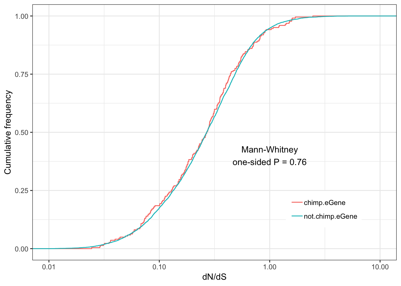
| Version | Author | Date |
|---|---|---|
| 22eda3a | Benjmain Fair | 2019-06-12 |
Chimp.identity.plot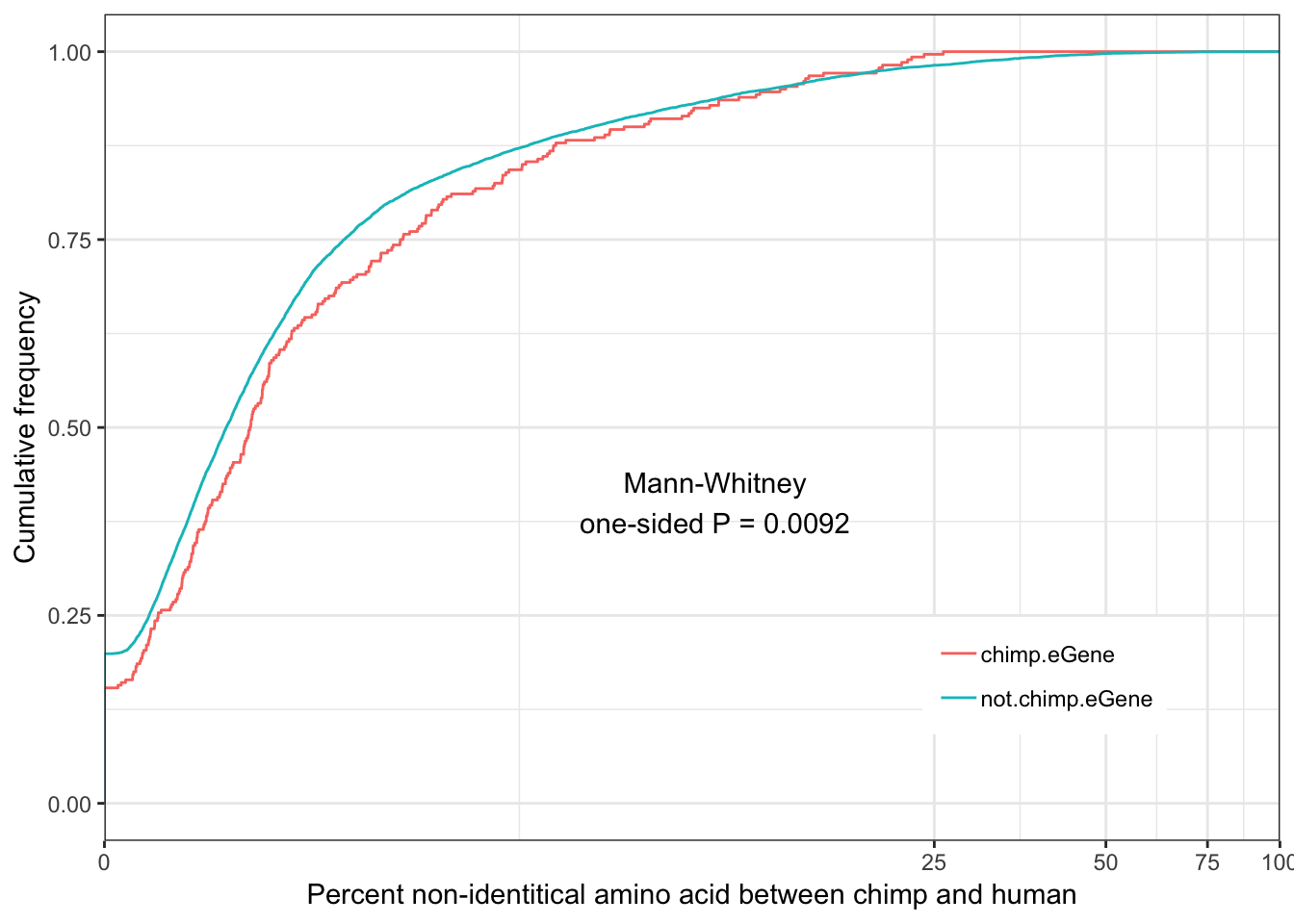
| Version | Author | Date |
|---|---|---|
| 22eda3a | Benjmain Fair | 2019-06-12 |
Human.dNdS.plotWarning: Transformation introduced infinite values in continuous x-axis
Warning: Removed 2951 rows containing non-finite values (stat_ecdf).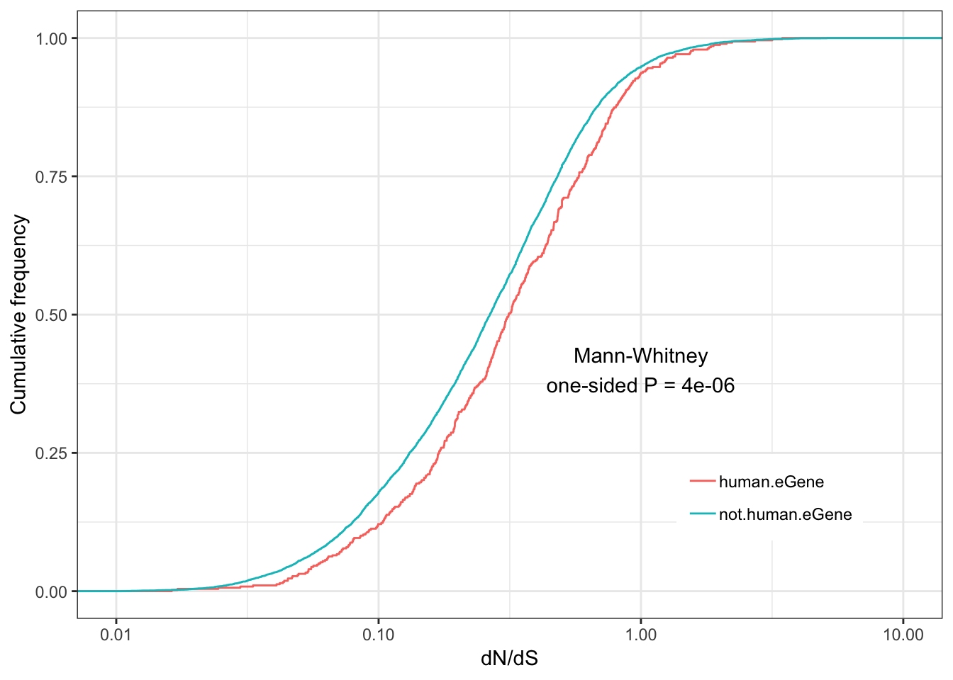
| Version | Author | Date |
|---|---|---|
| 22eda3a | Benjmain Fair | 2019-06-12 |
Human.identity.plot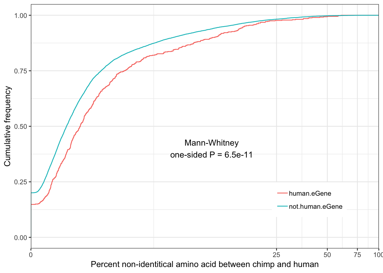
| Version | Author | Date |
|---|---|---|
| 22eda3a | Benjmain Fair | 2019-06-12 |
Shared.human.dNdS.plotWarning: Removed 122 rows containing non-finite values (stat_ecdf).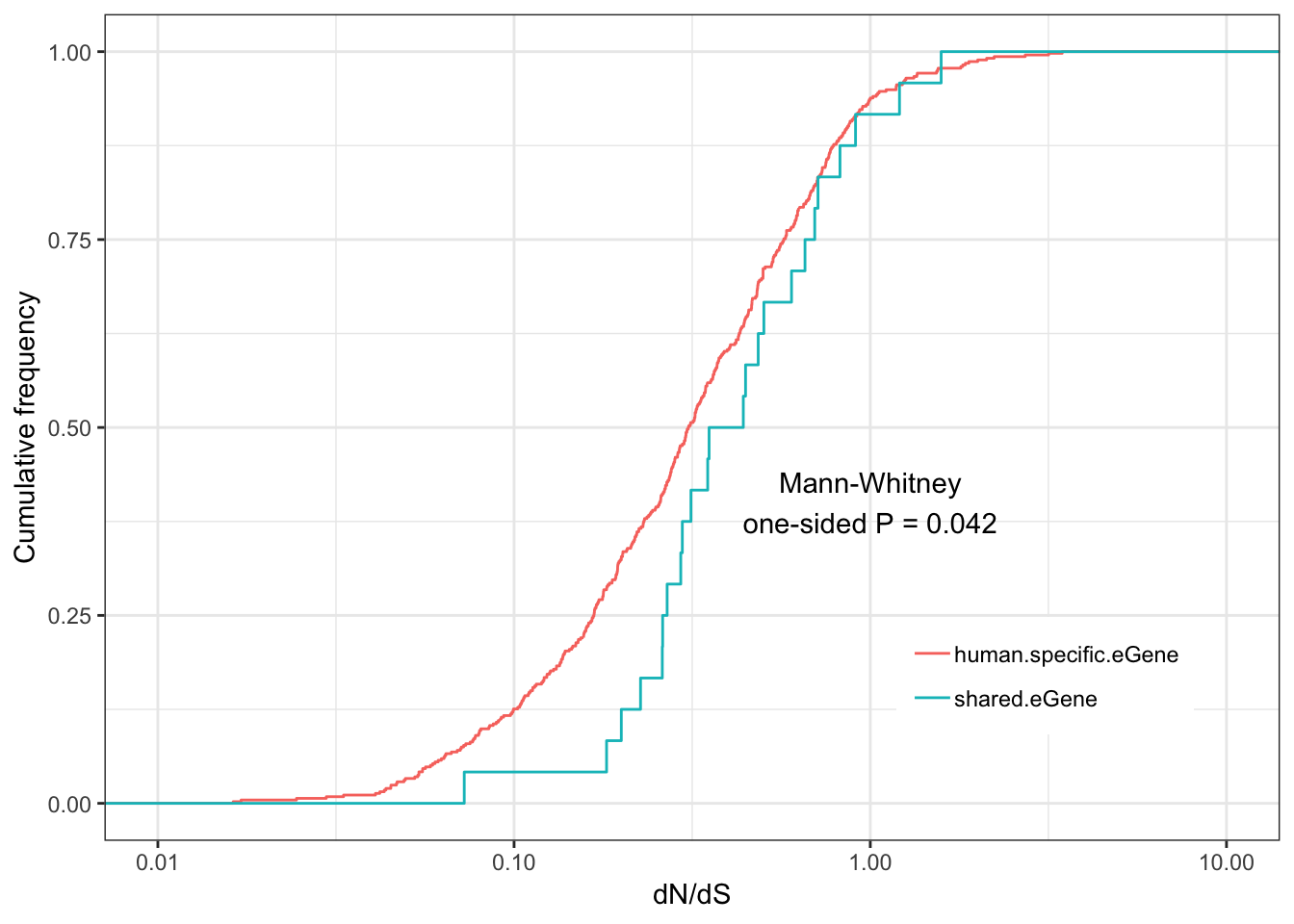
| Version | Author | Date |
|---|---|---|
| 22eda3a | Benjmain Fair | 2019-06-12 |
Shared.human.identity.plot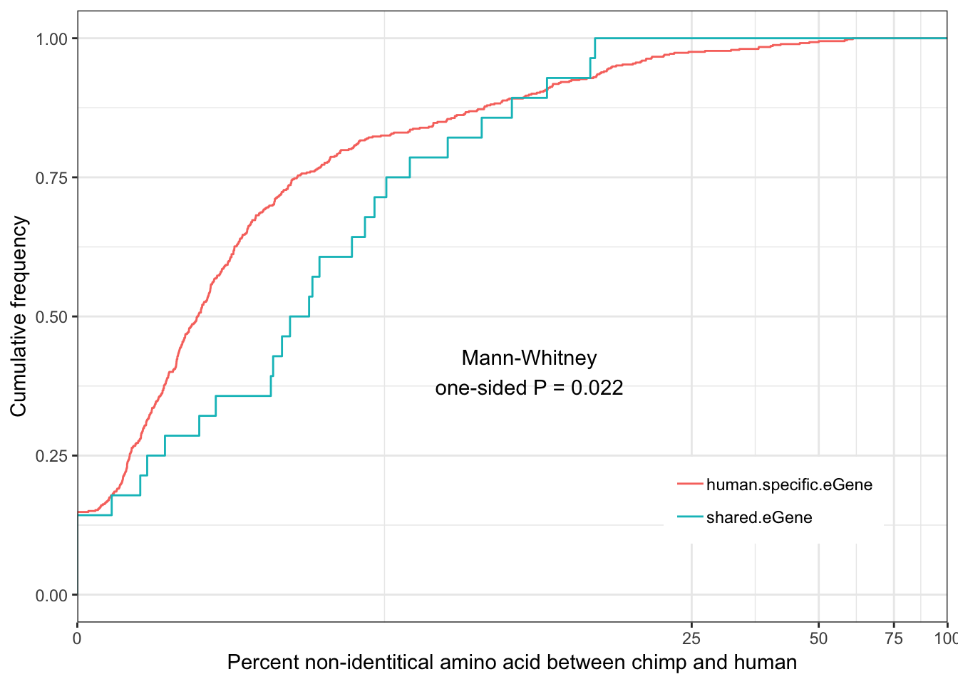
| Version | Author | Date |
|---|---|---|
| 22eda3a | Benjmain Fair | 2019-06-12 |
Shared.chimp.dNdS.plotWarning: Transformation introduced infinite values in continuous x-axisWarning: Removed 58 rows containing non-finite values (stat_ecdf).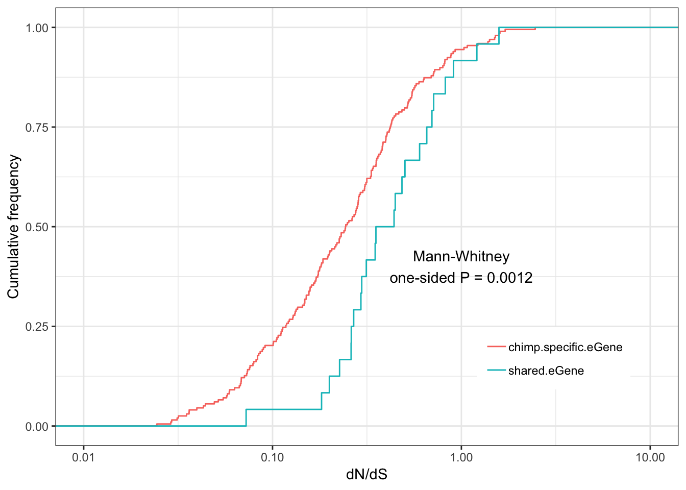
| Version | Author | Date |
|---|---|---|
| 22eda3a | Benjmain Fair | 2019-06-12 |
Shared.chimp.identity.plot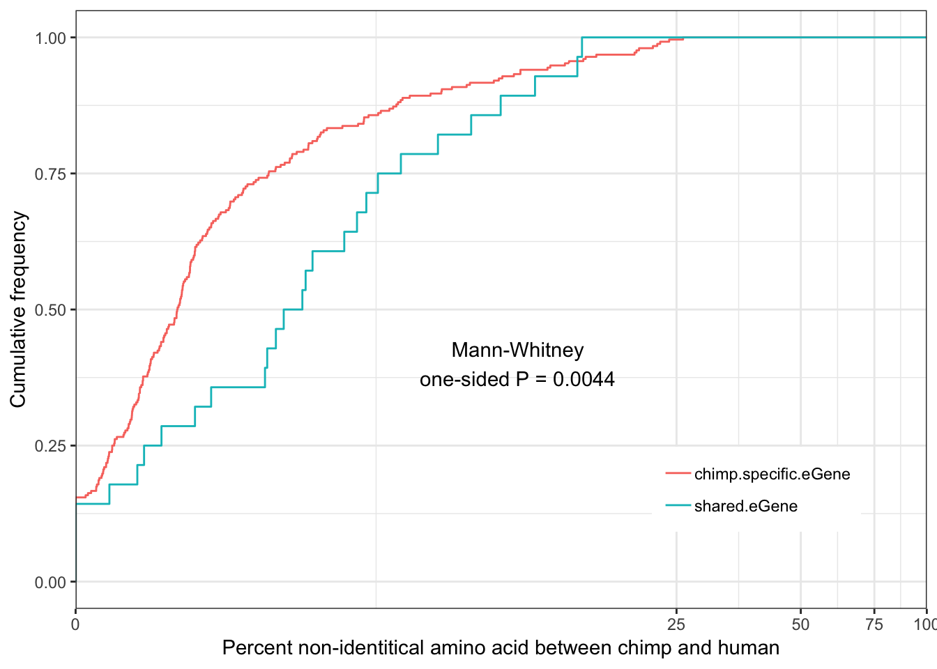
| Version | Author | Date |
|---|---|---|
| 22eda3a | Benjmain Fair | 2019-06-12 |
ToPlot <- GtexHeartEgenes %>%
  left_join(OneToOneMap, by=c("chimp_id"="Chimpanzee.gene.stable.ID"))
Some general and unsurprising conclusions:
eGenes are less conserved than non eGenes, and species shared eGenes are less conserved than species specific eGenes.
sessionInfo()R version 3.5.1 (2018-07-02)
Platform: x86_64-apple-darwin15.6.0 (64-bit)
Running under: macOS 10.14
Matrix products: default
BLAS: /Library/Frameworks/R.framework/Versions/3.5/Resources/lib/libRblas.0.dylib
LAPACK: /Library/Frameworks/R.framework/Versions/3.5/Resources/lib/libRlapack.dylib
locale:
[1] en_US.UTF-8/en_US.UTF-8/en_US.UTF-8/C/en_US.UTF-8/en_US.UTF-8
attached base packages:
[1] parallel stats4 stats graphics grDevices utils datasets
[8] methods base
other attached packages:
[1] gridExtra_2.3 org.Hs.eg.db_3.7.0 AnnotationDbi_1.44.0
[4] IRanges_2.16.0 S4Vectors_0.20.1 Biobase_2.42.0
[7] BiocGenerics_0.28.0 clusterProfiler_3.10.1 ggpmisc_0.3.1
[10] data.table_1.12.2 knitr_1.23 forcats_0.4.0
[13] stringr_1.4.0 dplyr_0.8.1 purrr_0.3.2
[16] readr_1.3.1 tidyr_0.8.3 tibble_2.1.3
[19] ggplot2_3.1.1 tidyverse_1.2.1 plyr_1.8.4
loaded via a namespace (and not attached):
[1] nlme_3.1-140 fs_1.3.1 enrichplot_1.2.0
[4] lubridate_1.7.4 bit64_0.9-7 progress_1.2.2
[7] RColorBrewer_1.1-2 httr_1.4.0 UpSetR_1.4.0
[10] rprojroot_1.3-2 tools_3.5.1 backports_1.1.4
[13] R6_2.4.0 DBI_1.0.0 lazyeval_0.2.2
[16] colorspace_1.4-1 withr_2.1.2 prettyunits_1.0.2
[19] tidyselect_0.2.5 bit_1.1-14 compiler_3.5.1
[22] git2r_0.25.2 cli_1.1.0 rvest_0.3.4
[25] xml2_1.2.0 labeling_0.3 triebeard_0.3.0
[28] scales_1.0.0 ggridges_0.5.1 digest_0.6.19
[31] rmarkdown_1.13 DOSE_3.8.2 pkgconfig_2.0.2
[34] htmltools_0.3.6 highr_0.8 rlang_0.3.4
[37] readxl_1.3.1 rstudioapi_0.10 RSQLite_2.1.1
[40] gridGraphics_0.4-1 generics_0.0.2 farver_1.1.0
[43] jsonlite_1.6 BiocParallel_1.16.6 GOSemSim_2.8.0
[46] magrittr_1.5 ggplotify_0.0.3 GO.db_3.7.0
[49] Matrix_1.2-17 Rcpp_1.0.1 munsell_0.5.0
[52] viridis_0.5.1 stringi_1.4.3 whisker_0.3-2
[55] yaml_2.2.0 ggraph_1.0.2 MASS_7.3-51.4
[58] qvalue_2.14.1 grid_3.5.1 blob_1.1.1
[61] ggrepel_0.8.1 DO.db_2.9 crayon_1.3.4
[64] lattice_0.20-38 cowplot_0.9.4 haven_2.1.0
[67] splines_3.5.1 hms_0.4.2 pillar_1.4.1
[70] fgsea_1.8.0 igraph_1.2.4.1 reshape2_1.4.3
[73] fastmatch_1.1-0 glue_1.3.1 evaluate_0.14
[76] modelr_0.1.4 urltools_1.7.3 tweenr_1.0.1
[79] cellranger_1.1.0 gtable_0.3.0 polyclip_1.10-0
[82] assertthat_0.2.1 xfun_0.7 ggforce_0.2.2
[85] europepmc_0.3 broom_0.5.2 viridisLite_0.3.0
[88] rvcheck_0.1.3 memoise_1.1.0 workflowr_1.4.0