20190617_ExpressionVarianceOfEgenes
Ben Fair
6/17/2019
Last updated: 2019-08-06
Checks: 7 0
Knit directory: Comparative_eQTL/analysis/
This reproducible R Markdown analysis was created with workflowr (version 1.4.0). The Checks tab describes the reproducibility checks that were applied when the results were created. The Past versions tab lists the development history.
Great! Since the R Markdown file has been committed to the Git repository, you know the exact version of the code that produced these results.
Great job! The global environment was empty. Objects defined in the global environment can affect the analysis in your R Markdown file in unknown ways. For reproduciblity it’s best to always run the code in an empty environment.
The command set.seed(20190319) was run prior to running the code in the R Markdown file. Setting a seed ensures that any results that rely on randomness, e.g. subsampling or permutations, are reproducible.
Great job! Recording the operating system, R version, and package versions is critical for reproducibility.
Nice! There were no cached chunks for this analysis, so you can be confident that you successfully produced the results during this run.
Great job! Using relative paths to the files within your workflowr project makes it easier to run your code on other machines.
Great! You are using Git for version control. Tracking code development and connecting the code version to the results is critical for reproducibility. The version displayed above was the version of the Git repository at the time these results were generated.
Note that you need to be careful to ensure that all relevant files for the analysis have been committed to Git prior to generating the results (you can use wflow_publish or wflow_git_commit). workflowr only checks the R Markdown file, but you know if there are other scripts or data files that it depends on. Below is the status of the Git repository when the results were generated:
Ignored files:
    Ignored:    .DS_Store
    Ignored:    .Rhistory
    Ignored:    .Rproj.user/
    Ignored:    analysis/.DS_Store
    Ignored:    analysis/20190521_eQTL_CrossSpeciesEnrichment_cache/
    Ignored:    analysis_temp/.DS_Store
    Ignored:    code/.DS_Store
    Ignored:    code/snakemake_workflow/.DS_Store
    Ignored:    code/snakemake_workflow/rules/.eQTL_analysis.smk.swp
    Ignored:    data/.DS_Store
    Ignored:    data/PastAnalysesDataToKeep/.DS_Store
    Ignored:    docs/.DS_Store
    Ignored:    docs/assets/.DS_Store

Unstaged changes:
    Modified:   analysis/20190521_eQTL_CrossSpeciesEnrichment.Rmd
    Modified:   analysis/20190627_DiffContactsEgenes.Rmd
    Modified:   analysis/20190708_DiffContactsEgenes_CisWindowControlled.Rmd
    Modified:   analysis/20190716_VarianceInsteadOfEgenes.Rmd
    Modified:   analysis/index.Rmd
    Modified:   code/snakemake_workflow/Session.vim
    Modified:   code/snakemake_workflow/rules/eQTL_analysis.smk
Note that any generated files, e.g. HTML, png, CSS, etc., are not included in this status report because it is ok for generated content to have uncommitted changes.
These are the previous versions of the R Markdown and HTML files. If you’ve configured a remote Git repository (see ?wflow_git_remote), click on the hyperlinks in the table below to view them.
| File | Version | Author | Date | Message |
|---|---|---|---|---|
| Rmd | c3dbe5a | Benjmain Fair | 2019-06-19 | update site |
| html | c3dbe5a | Benjmain Fair | 2019-06-19 | update site |
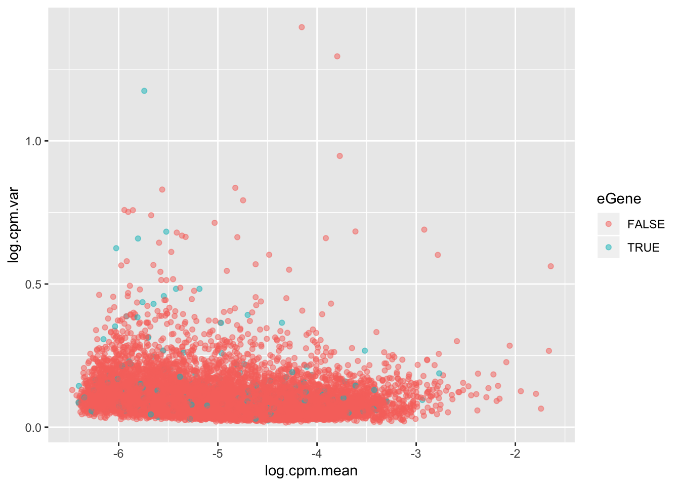
For my own understanding of what it means to be an eGene, I wanted to plot from my chimp data the variance in expression levels of eGenes vs non eGenes. This is an important component to if it is reasonable to intepret eGene character as a proxy for stabilizing selection and/or low expression variance genes.
The way I will go about this is looking at the original count table of CPM for all tested genes, and plot the mean/variance trend with eGenes as a different color.
library(tidyverse)

eQTLs <- read.table("../output/MatrixEQTL_sig_eqtls.txt", header=T)
CountTable <- as.matrix(read.table("../output/ExpressionMatrix.un-normalized.txt.gz", header=T))

ToPlot <- as.data.frame(CountTable) %>%
  rownames_to_column("gene") %>%
  mutate(log.cpm.mean=apply(CountTable,1,mean),
         log.cpm.var=apply(CountTable,1,var),
         eGene=(gene %in% eQTLs$gene)) %>%
  mutate(CV=log.cpm.mean/sqrt(log.cpm.var))

ToPlot %>%
  ggplot(aes(x=log.cpm.mean, y=log.cpm.var, color=eGene)) +
  geom_point(alpha=0.5)
| Version | Author | Date |
|---|---|---|
| c3dbe5a | Benjmain Fair | 2019-06-19 |
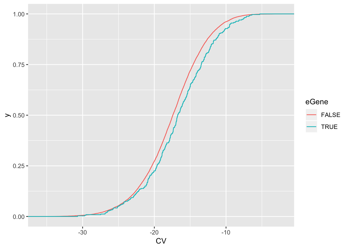
Maybe a different way to look at this trend will be more clear
wilcox.test(data=ToPlot, CV ~ eGene)
    Wilcoxon rank sum test with continuity correction

data:  CV by eGene
W = 1964800, p-value = 0.0008523
alternative hypothesis: true location shift is not equal to 0
ToPlot %>%
ggplot(aes(x=CV, color=eGene)) +
stat_ecdf(geom = "step")
| Version | Author | Date |
|---|---|---|
| c3dbe5a | Benjmain Fair | 2019-06-19 |
eGenes have higher coefficient of variation
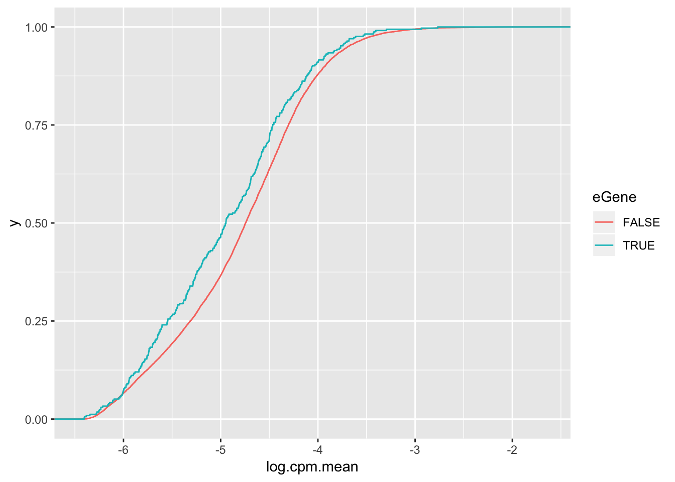
wilcox.test(data=ToPlot, log.cpm.mean ~ eGene)
    Wilcoxon rank sum test with continuity correction

data:  log.cpm.mean by eGene
W = 2470400, p-value = 0.0001234
alternative hypothesis: true location shift is not equal to 0
ToPlot %>%
ggplot(aes(x=log.cpm.mean, color=eGene)) +
stat_ecdf(geom = "step")
| Version | Author | Date |
|---|---|---|
| c3dbe5a | Benjmain Fair | 2019-06-19 |
but actually lower expression level
But all being said, the effect size is to the point where eGene character I think is only modest evidence for lack of stabilizing selection. Maybe the thing to do is to check the correlation between selection on coding regions (dN/dS or percent identity between two species) and the variance within a species to see if that signal is stronger than for eGene character.
ChimpToHumanGeneMap <- read.table("../data/Biomart_export.Hsap.Ptro.orthologs.txt.gz", header=T, sep='\t', stringsAsFactors = F)

# Of this ortholog list, how many genes are one2one
table(ChimpToHumanGeneMap$Chimpanzee.homology.type)
ortholog_many2many  ortholog_one2many   ortholog_one2one
              2278              19917             140351
OneToOneMap <- ChimpToHumanGeneMap %>%
filter(Chimpanzee.homology.type=="ortholog_one2one") %>%
distinct(Chimpanzee.gene.stable.ID, .keep_all = TRUE)
ChimpToHuman.ID <- function(Chimp.ID){
#function to convert chimp ensembl to human ensembl gene ids
return(
plyr::mapvalues(Chimp.ID, OneToOneMap$Chimpanzee.gene.stable.ID, OneToOneMap$Gene.stable.ID, warn_missing = F)
)}
ToPlotAdded <- ToPlot %>%
left_join(OneToOneMap, by=c("gene"="Chimpanzee.gene.stable.ID")) %>%
mutate(dN.dS = dN.with.Chimpanzee/dS.with.Chimpanzee,
rank = dense_rank(desc(CV))) %>%
mutate(TopN.Var.Genes=rank<300) %>%
ggplot(aes(x=100-X.id..query.gene.identical.to.target.Chimpanzee.gene, color=TopN.Var.Genes)) +
stat_ecdf(geom = "step") +
scale_x_continuous(trans='log1p')Surprising to me, chimp expression coefficient of variation (n=39) doesn’t separate dN/dS or percent identity better than chimp eGene classificiation. There are a couple things I should probably change about the above analysis to make it a more fair comparison to the eGene classificiation: I should be considering variation in TPM
sessionInfo()R version 3.5.1 (2018-07-02)
Platform: x86_64-apple-darwin15.6.0 (64-bit)
Running under: macOS 10.14
Matrix products: default
BLAS: /Library/Frameworks/R.framework/Versions/3.5/Resources/lib/libRblas.0.dylib
LAPACK: /Library/Frameworks/R.framework/Versions/3.5/Resources/lib/libRlapack.dylib
locale:
[1] en_US.UTF-8/en_US.UTF-8/en_US.UTF-8/C/en_US.UTF-8/en_US.UTF-8
attached base packages:
[1] stats graphics grDevices utils datasets methods base
other attached packages:
[1] forcats_0.4.0 stringr_1.4.0 dplyr_0.8.1 purrr_0.3.2
[5] readr_1.3.1 tidyr_0.8.3 tibble_2.1.3 ggplot2_3.1.1
[9] tidyverse_1.2.1
loaded via a namespace (and not attached):
[1] Rcpp_1.0.1 cellranger_1.1.0 plyr_1.8.4 pillar_1.4.1
[5] compiler_3.5.1 git2r_0.25.2 workflowr_1.4.0 tools_3.5.1
[9] digest_0.6.19 lubridate_1.7.4 jsonlite_1.6 evaluate_0.14
[13] nlme_3.1-140 gtable_0.3.0 lattice_0.20-38 pkgconfig_2.0.2
[17] rlang_0.3.4 cli_1.1.0 rstudioapi_0.10 yaml_2.2.0
[21] haven_2.1.0 xfun_0.7 withr_2.1.2 xml2_1.2.0
[25] httr_1.4.0 knitr_1.23 hms_0.4.2 generics_0.0.2
[29] fs_1.3.1 rprojroot_1.3-2 grid_3.5.1 tidyselect_0.2.5
[33] glue_1.3.1 R6_2.4.0 readxl_1.3.1 rmarkdown_1.13
[37] modelr_0.1.4 magrittr_1.5 whisker_0.3-2 backports_1.1.4
[41] scales_1.0.0 htmltools_0.3.6 rvest_0.3.4 assertthat_0.2.1
[45] colorspace_1.4-1 labeling_0.3 stringi_1.4.3 lazyeval_0.2.2
[49] munsell_0.5.0 broom_0.5.2 crayon_1.3.4