Check RNA-seq PCs
Ben Fair
3/20/2019
Last updated: 2019-07-24
Checks: 7 0
Knit directory: Comparative_eQTL/analysis/
This reproducible R Markdown analysis was created with workflowr (version 1.4.0). The Checks tab describes the reproducibility checks that were applied when the results were created. The Past versions tab lists the development history.
Great! Since the R Markdown file has been committed to the Git repository, you know the exact version of the code that produced these results.
Great job! The global environment was empty. Objects defined in the global environment can affect the analysis in your R Markdown file in unknown ways. For reproduciblity it’s best to always run the code in an empty environment.
The command set.seed(20190319) was run prior to running the code in the R Markdown file. Setting a seed ensures that any results that rely on randomness, e.g. subsampling or permutations, are reproducible.
Great job! Recording the operating system, R version, and package versions is critical for reproducibility.
Nice! There were no cached chunks for this analysis, so you can be confident that you successfully produced the results during this run.
Great job! Using relative paths to the files within your workflowr project makes it easier to run your code on other machines.
Great! You are using Git for version control. Tracking code development and connecting the code version to the results is critical for reproducibility. The version displayed above was the version of the Git repository at the time these results were generated.
Note that you need to be careful to ensure that all relevant files for the analysis have been committed to Git prior to generating the results (you can use wflow_publish or wflow_git_commit). workflowr only checks the R Markdown file, but you know if there are other scripts or data files that it depends on. Below is the status of the Git repository when the results were generated:
Ignored files:
    Ignored:    .DS_Store
    Ignored:    .Rhistory
    Ignored:    .Rproj.user/
    Ignored:    analysis/.DS_Store
    Ignored:    analysis/20190521_eQTL_CrossSpeciesEnrichment_cache/
    Ignored:    analysis_temp/.DS_Store
    Ignored:    code/.DS_Store
    Ignored:    code/snakemake_workflow/.DS_Store
    Ignored:    data/.DS_Store
    Ignored:    data/PastAnalysesDataToKeep/.DS_Store
    Ignored:    docs/.DS_Store
    Ignored:    docs/assets/.DS_Store

Untracked files:
    Untracked:  GSEA_eQTL.pdf
    Untracked:  Rplot01.pdf

Unstaged changes:
    Modified:   analysis/20190521_eQTL_CrossSpeciesEnrichment.Rmd
    Modified:   analysis/20190613_PowerAnalysis.Rmd
    Modified:   analysis/20190708_DiffContactsEgenes_CisWindowControlled.Rmd
    Modified:   analysis/20190716_VarianceInsteadOfEgenes.Rmd
Note that any generated files, e.g. HTML, png, CSS, etc., are not included in this status report because it is ok for generated content to have uncommitted changes.
These are the previous versions of the R Markdown and HTML files. If you’ve configured a remote Git repository (see ?wflow_git_remote), click on the hyperlinks in the table below to view them.
| File | Version | Author | Date | Message |
|---|---|---|---|---|
| Rmd | f469d6a | Benjmain Fair | 2019-07-16 | new analyses |
| Rmd | e592335 | Benjmain Fair | 2019-04-03 | build site |
| html | e592335 | Benjmain Fair | 2019-04-03 | build site |
library(plyr)
library(reshape2)
library(tidyverse)
library(readxl)
library(knitr)
library(ggrepel)
# Read in kinship data
YerkesKinship_from_pedigree <- as.data.frame(read_excel("../data/Metadata.xlsx", sheet="Yerkes.coan", col_types = c("text", "text", "numeric")))
kable(head(YerkesKinship_from_pedigree))| ind1 | ind2 | coeff |
|---|---|---|
| 200 | 200 | 0.5 |
| 204 | 200 | 0.0 |
| 295 | 200 | 0.0 |
| 299 | 200 | 0.0 |
| 317 | 200 | 0.0 |
| 338 | 200 | 0.0 |
Kinship_from_KING.WGS <- read.table("../output/PopulationStructure/king.kin", header=T, stringsAsFactors = F)
kable(head(Kinship_from_KING.WGS))| FID | ID1 | ID2 | N_SNP | Z0 | Phi | HetHet | IBS0 | Kinship | Error |
|---|---|---|---|---|---|---|---|---|---|
| Pan_troglodytes_ThisStudy | Little_R | MD_And | 4901461 | 1 | 0 | 0.042 | 0.0277 | -0.0526 | 0 |
| Pan_troglodytes_ThisStudy | Little_R | 4x373 | 4901461 | 1 | 0 | 0.045 | 0.0255 | -0.0250 | 0 |
| Pan_troglodytes_ThisStudy | Little_R | 4x523 | 4901461 | 1 | 0 | 0.046 | 0.0269 | -0.0206 | 0 |
| Pan_troglodytes_ThisStudy | Little_R | 4x0025 | 4901461 | 1 | 0 | 0.044 | 0.0262 | -0.0325 | 0 |
| Pan_troglodytes_ThisStudy | Little_R | 4x0043 | 4901461 | 1 | 0 | 0.043 | 0.0281 | -0.0548 | 0 |
| Pan_troglodytes_ThisStudy | Little_R | 4X0095 | 4901461 | 1 | 0 | 0.042 | 0.0296 | -0.0702 | 0 |
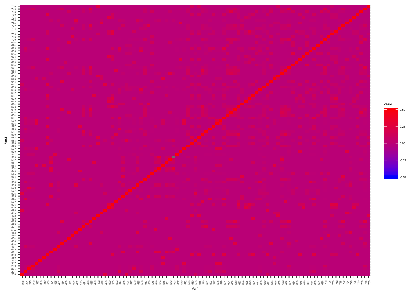
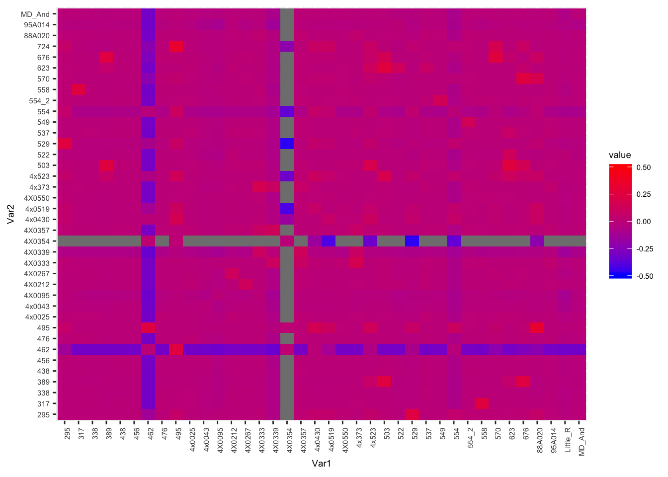
| Plot the kinship matrix obta | ined from Y | erkes ped | igree data | , as | well a | s the mat | rix obtai | ned from w | hole genome SNP data… |
Yerkes.Matrix <-acast(YerkesKinship_from_pedigree, ind1 ~ ind2, value.var="coeff", fill=0)
melt(Yerkes.Matrix) %>%
  ggplot(aes(x=Var1, y=Var2, fill=value)) +
    geom_tile() +
    scale_fill_gradient(low="blue", high="red", limits=c(-0.5, 0.5)) +
    theme(text = element_text(size=4), axis.text.x = element_text(angle=90, hjust=1))
| Version | Author | Date |
|---|---|---|
| e592335 | Benjmain Fair | 2019-04-03 |
WGS.Matrix <- acast(Kinship_from_KING.WGS, ID1 ~ ID2, value.var="Kinship", fill=0) + acast(Kinship_from_KING.WGS, ID2 ~ ID1, value.var="Kinship", fill=0)
melt(WGS.Matrix) %>%
  ggplot(aes(x=Var1, y=Var2, fill=value)) +
    geom_tile() +
    scale_fill_gradient(low="blue", high="red", limits=c(-0.5, 0.5)) +
    theme(text = element_text(size=7), axis.text.x = element_text(angle=90, hjust=1))
| Version | Author | Date |
|---|---|---|
| e592335 | Benjmain Fair | 2019-04-03 |
Let’s fix a known sample mislabel… 554_2 is actually 554. And 554 is actually unknown.
Kinship_from_KING.WGS$ID1 <- mapvalues(Kinship_from_KING.WGS$ID1, from=c("554_2"), to=c("554"))
Kinship_from_KING.WGS$ID2 <- mapvalues(Kinship_from_KING.WGS$ID2, from=c("554_2"), to=c("554"))
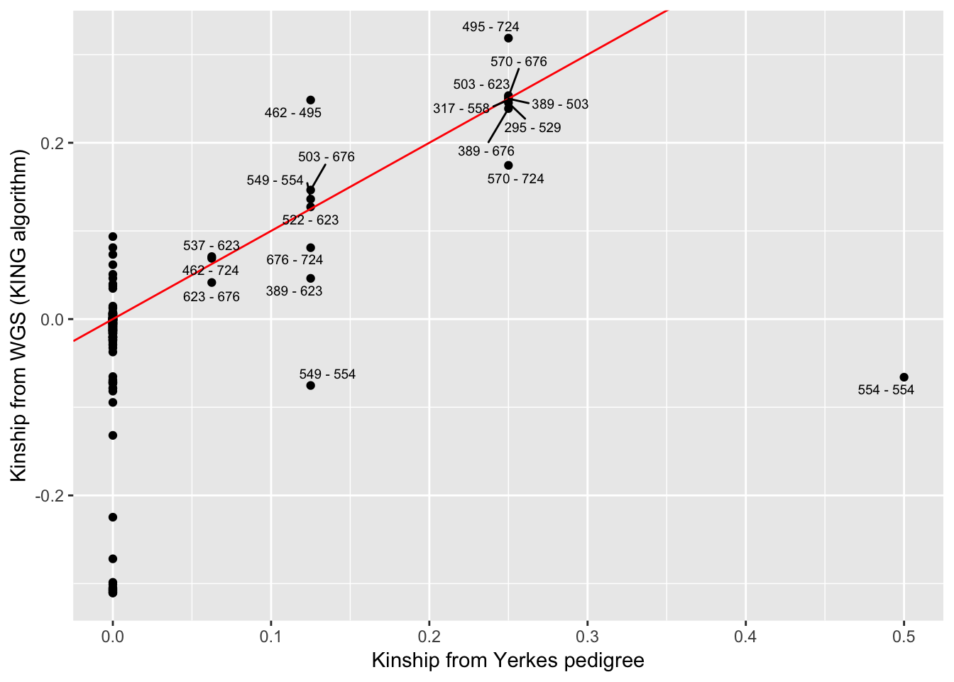
Now I want to correlate the kinship-coefficients from Yerkes pedigree to those from the whole genome SNP data (KING algorithm). Easiest way I could think to match up the pairwise kinship coefficients is to make a new field that is the sorted ID pair and then merge the Yerkes coefficient-table to the KING-table by the sorted ID pairs…
KSort <- Kinship_from_KING.WGS %>%
  mutate(Teams = paste(pmin(ID1, ID2), pmax(ID1, ID2), sep= " - "))
YSort <- YerkesKinship_from_pedigree %>%
  mutate(Teams = paste(pmin(ind1, ind2), pmax(ind1, ind2), sep= " - ")) %>%
  distinct(Teams, .keep_all=T)
# Merge and plot
Merged <- merge(KSort, YSort, by="Teams")
Merged$label <- Merged$Team
Merged$label[Merged$coeff==0] <- ""

ggplot(Merged, aes(x=coeff, y=Kinship, label=label)) +
  geom_point() +
  geom_abline(slope=1, intercept=0, color="red") +
  geom_text_repel(size=2.5) +
  xlab("Kinship from Yerkes pedigree") +
  ylab("Kinship from WGS (KING algorithm)")
| Version | Author | Date |
|---|---|---|
| e592335 | Benjmain Fair | 2019-04-03 |
# geom_jitter()The expected value of Kinships coefficients from KING seem to match pedigree info, with the exception of sample 554 (not to be confused with 554_2 which for purposes of matching KING coefficients to pedigree coefficients we relabelled as 554) which we had prior knowledge to be a mislabelled sample… Hence why 554 is unrelated to a point labelled 554 (actually 554_2). Assuming sample 554 came from Yerkes, we might be able to correlate its kinship coefficients to other Yerkes chimps to help identify it. Bryan Pavlovic already did this for me by looking at the kinship matrices by hand and concluded that 554 is most likely Booka, but here I will repeat that analysis…
# Find who 554 is related to from whole genome SNP data.
WGS.Matrix['554',] %>%
  sort(decreasing=T) %>%
  head() %>%
t() %>% kable()| 495 | 4x0430 | 295 | 4x0519 | 529 | 4x523 |
|---|---|---|---|---|---|
| 0.0936 | 0.0561 | 0.0463 | 0.0356 | 0.0348 | 0.0328 |
| …554 lo | oks relat | ed to 495 | (Amos), | perhaps 2 | nd or 3rd degree relationship |
# Find who to Amos is related from Yerkes Pedigree
Yerkes.Matrix['495',] %>%
  sort(decreasing=T) %>%
  head(20) %>%
t() %>% kable()| 495 | 724 | 462 | 646 | 650 | 535 | 726 | 200 | 204 | 295 | 299 | 317 | 338 | 380 | 389 | 421 | 425 | 431 | 434 | 438 |
|---|---|---|---|---|---|---|---|---|---|---|---|---|---|---|---|---|---|---|---|
| 0.5 | 0.25 | 0.125 | 0.125 | 0.125 | 0.0625 | 0.0625 | 0 | 0 | 0 | 0 | 0 | 0 | 0 | 0 | 0 | 0 | 0 | 0 | 0 |
| Can el | iminate | 495, 72 | 4, 462 a | s they a | re all al | so part o | f my c | ohort, | and n | ot rel | ated t | o 554. |
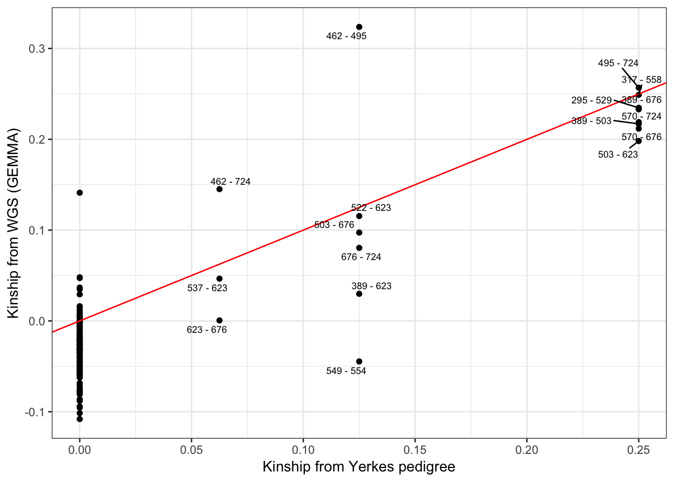
Update for presentation:
make same scatter plot (kinship estimated from wgs vs kinship from pedigree) based on the gemma-derived kinship matrix that i actually used for eqtl calling
SampleLabels <- read.table('../output/ForAssociationTesting.temp.fam', stringsAsFactors = F)$V2
GemmaMatrix <- as.matrix(read.table('../output/GRM.cXX.txt'))
colnames(GemmaMatrix) <- SampleLabels
row.names(GemmaMatrix) <- SampleLabels

KSort <- melt(GemmaMatrix) %>%
  mutate(ID1=as.character(Var1), ID2=as.character(Var2)) %>%
  mutate(Teams = paste(pmin(ID1, ID2), pmax(ID1, ID2), sep= " - ")) %>%
  distinct(Teams, .keep_all=T)
YSort <- YerkesKinship_from_pedigree %>%
  mutate(Teams = paste(pmin(ind1, ind2), pmax(ind1, ind2), sep= " - ")) %>%
  distinct(Teams, .keep_all=T)
# Merge and plot
Merged <- merge(KSort, YSort, by="Teams")
Merged$label <- Merged$Team
Merged$label[Merged$coeff==0] <- ""

Merged %>%
  filter(!ID1==ID2) %>%
ggplot(aes(x=coeff, y=value*2, label=label)) +
  geom_point() +
  geom_abline(slope=1, intercept=0, color="red") +
  geom_text_repel(size=2.5) +
  xlab("Kinship from Yerkes pedigree") +
  ylab("Kinship from WGS (GEMMA)") +
  theme_bw()
# geom_jitter()
sessionInfo()R version 3.5.1 (2018-07-02)
Platform: x86_64-apple-darwin15.6.0 (64-bit)
Running under: macOS 10.14
Matrix products: default
BLAS: /Library/Frameworks/R.framework/Versions/3.5/Resources/lib/libRblas.0.dylib
LAPACK: /Library/Frameworks/R.framework/Versions/3.5/Resources/lib/libRlapack.dylib
locale:
[1] en_US.UTF-8/en_US.UTF-8/en_US.UTF-8/C/en_US.UTF-8/en_US.UTF-8
attached base packages:
[1] stats graphics grDevices utils datasets methods base
other attached packages:
[1] ggrepel_0.8.1 knitr_1.23 readxl_1.3.1 forcats_0.4.0
[5] stringr_1.4.0 dplyr_0.8.1 purrr_0.3.2 readr_1.3.1
[9] tidyr_0.8.3 tibble_2.1.3 ggplot2_3.1.1 tidyverse_1.2.1
[13] reshape2_1.4.3 plyr_1.8.4
loaded via a namespace (and not attached):
[1] tidyselect_0.2.5 xfun_0.7 haven_2.1.0 lattice_0.20-38
[5] colorspace_1.4-1 generics_0.0.2 htmltools_0.3.6 yaml_2.2.0
[9] rlang_0.3.4 pillar_1.4.1 glue_1.3.1 withr_2.1.2
[13] modelr_0.1.4 munsell_0.5.0 gtable_0.3.0 workflowr_1.4.0
[17] cellranger_1.1.0 rvest_0.3.4 evaluate_0.14 labeling_0.3
[21] highr_0.8 broom_0.5.2 Rcpp_1.0.1 scales_1.0.0
[25] backports_1.1.4 jsonlite_1.6 fs_1.3.1 hms_0.4.2
[29] digest_0.6.19 stringi_1.4.3 grid_3.5.1 rprojroot_1.3-2
[33] cli_1.1.0 tools_3.5.1 magrittr_1.5 lazyeval_0.2.2
[37] crayon_1.3.4 whisker_0.3-2 pkgconfig_2.0.2 xml2_1.2.0
[41] lubridate_1.7.4 assertthat_0.2.1 rmarkdown_1.13 httr_1.4.0
[45] rstudioapi_0.10 R6_2.4.0 nlme_3.1-140 git2r_0.25.2
[49] compiler_3.5.1