20190424_Check_eQTLs
Last updated: 2019-05-02
Checks: 5 1
Knit directory: Comparative_eQTL/analysis/
This reproducible R Markdown analysis was created with workflowr (version 1.2.0). The Report tab describes the reproducibility checks that were applied when the results were created. The Past versions tab lists the development history.
The R Markdown file has unstaged changes. To know which version of the R Markdown file created these results, you’ll want to first commit it to the Git repo. If you’re still working on the analysis, you can ignore this warning. When you’re finished, you can run wflow_publish to commit the R Markdown file and build the HTML.
Great job! The global environment was empty. Objects defined in the global environment can affect the analysis in your R Markdown file in unknown ways. For reproduciblity it’s best to always run the code in an empty environment.
The command set.seed(20190319) was run prior to running the code in the R Markdown file. Setting a seed ensures that any results that rely on randomness, e.g. subsampling or permutations, are reproducible.
Great job! Recording the operating system, R version, and package versions is critical for reproducibility.
Nice! There were no cached chunks for this analysis, so you can be confident that you successfully produced the results during this run.
Great! You are using Git for version control. Tracking code development and connecting the code version to the results is critical for reproducibility. The version displayed above was the version of the Git repository at the time these results were generated.
Note that you need to be careful to ensure that all relevant files for the analysis have been committed to Git prior to generating the results (you can use wflow_publish or wflow_git_commit). workflowr only checks the R Markdown file, but you know if there are other scripts or data files that it depends on. Below is the status of the Git repository when the results were generated:
Ignored files:
    Ignored:    .DS_Store
    Ignored:    .Rhistory
    Ignored:    .Rproj.user/
    Ignored:    analysis/.DS_Store
    Ignored:    analysis_temp/.DS_Store
    Ignored:    data/.DS_Store
    Ignored:    data/PastAnalysesDataToKeep/.DS_Store
    Ignored:    docs/.DS_Store

Untracked files:
    Untracked:  analysis/20190502_Check_eQTLs.Rmd
    Untracked:  analysis_temp/20190412_Check_eQTLs.Rmd
    Untracked:  data/PastAnalysesDataToKeep/20190428_log10TPM.txt.gz
    Untracked:  docs/assets/
    Untracked:  docs/figure/20190426_CheckRNASeqPCs_2.Rmd/
    Untracked:  docs/figure/20190429_RNASeqSTAR_quantifications.Rmd/
    Untracked:  docs/figure/20190502_Check_eQTLs.Rmd/

Unstaged changes:
    Deleted:    analysis/20190412_Check_eQTLs.Rmd
    Modified:   analysis/20190428_Check_eQTLs.Rmd
Note that any generated files, e.g. HTML, png, CSS, etc., are not included in this status report because it is ok for generated content to have uncommitted changes.
These are the previous versions of the R Markdown and HTML files. If you’ve configured a remote Git repository (see ?wflow_git_remote), click on the hyperlinks in the table below to view them.
| File | Version | Author | Date | Message |
|---|---|---|---|---|
| Rmd | ece3b4a | Benjmain Fair | 2019-04-30 | added STAR v kallisto comparison |
library(tidyverse)
library(knitr)
library(data.table)
My second pass at eqtl mapping was as follows: Genotypes filtered for MAF>0.5 & GenotypingRate>0.9, HWE-pvalue<10e-7.5. ~9.5M variants passed these filter. Gene expression as log(TPM), filtering for genes with >0 TPM (transcript level TPM summed to get gene TPM) in all samples (~14000 genes passed this filter). TPM was then standardized across individuals and quantile normalized to a normal distribution across genes. Sample MD_And was dropped from analysis because it was previously shown to be an outlier that caused spurious associations. Association testing used the following linear mixed model for each cis-variant-gene-pair (cis definied as <1Mb from gene):
\[ Y =Wα+xβ+u+ε \]
where \(Y\) is gene expression as \(log(TPM)\), \(W\) covariates include first three genotype principal components (to account for population structure) as well as 3 RNA-seq PCs, Sex, an interceptm and 3 genotype PCs. \(x\) is coded as 0,1,2, \(U \sim MVN(0,\sigma^2 K)\) where \(K\) an centered kinship matrix made from gemma software.
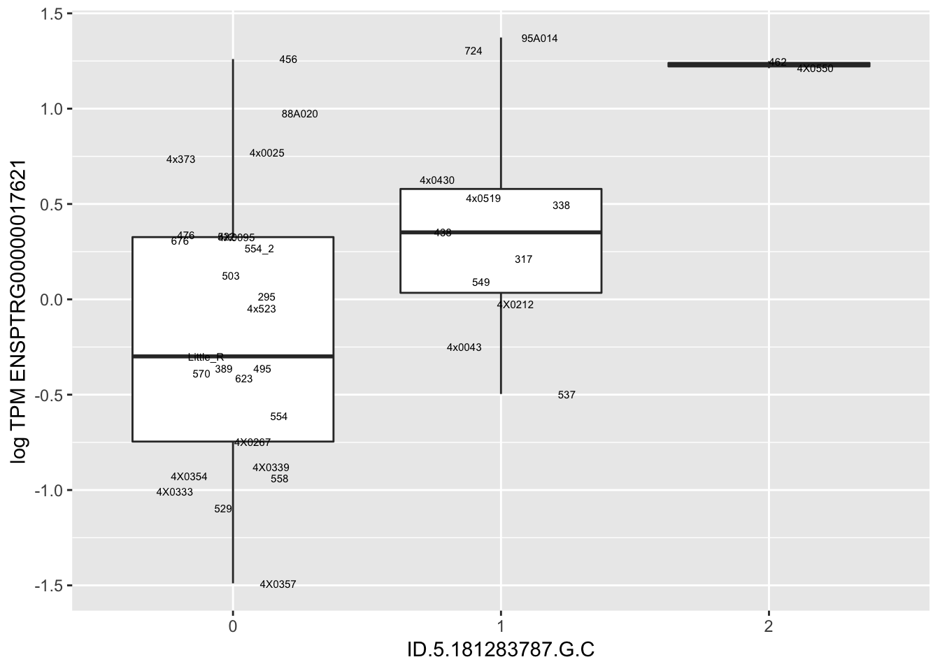
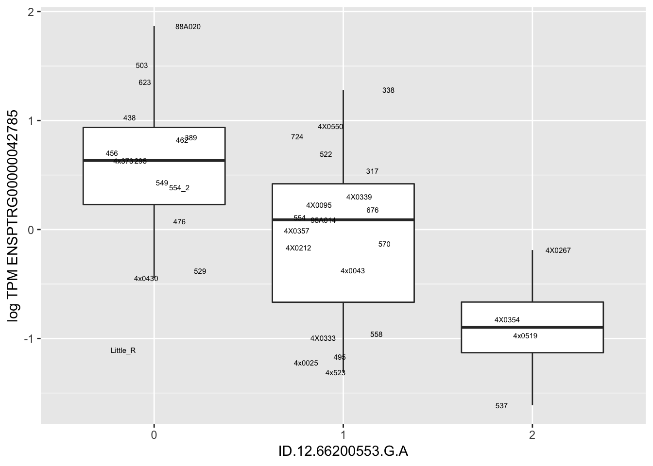
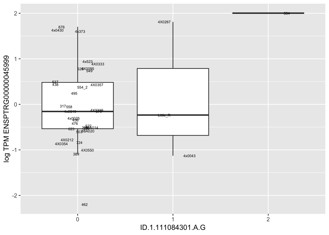
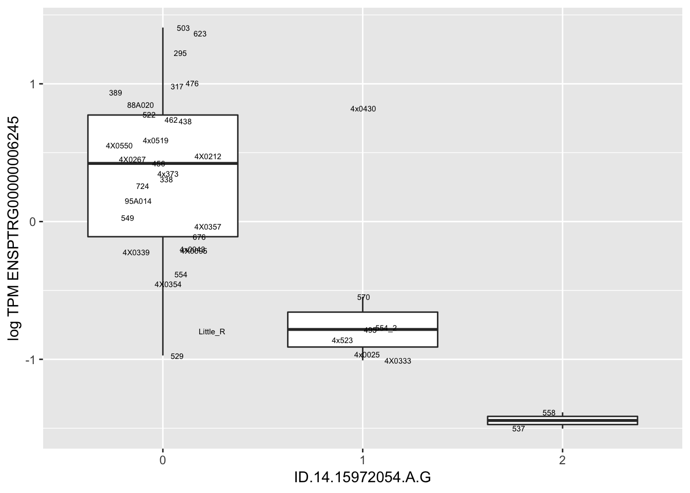
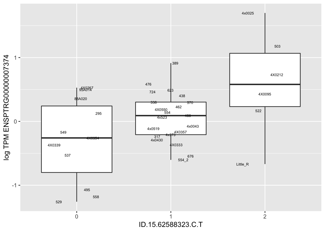
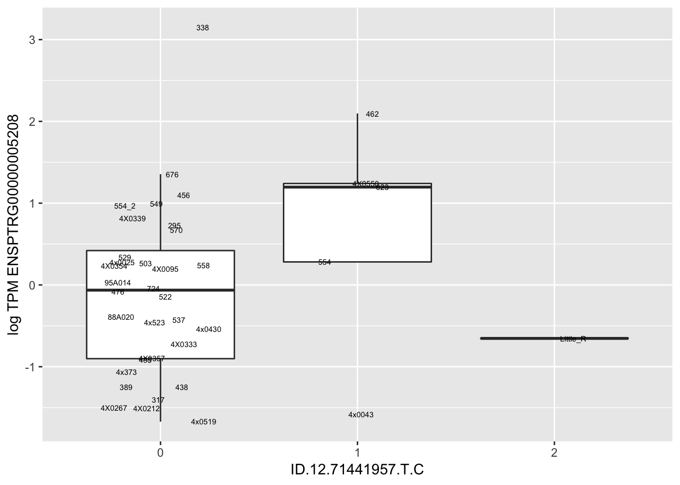
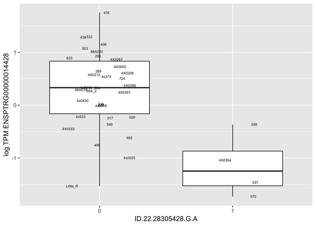
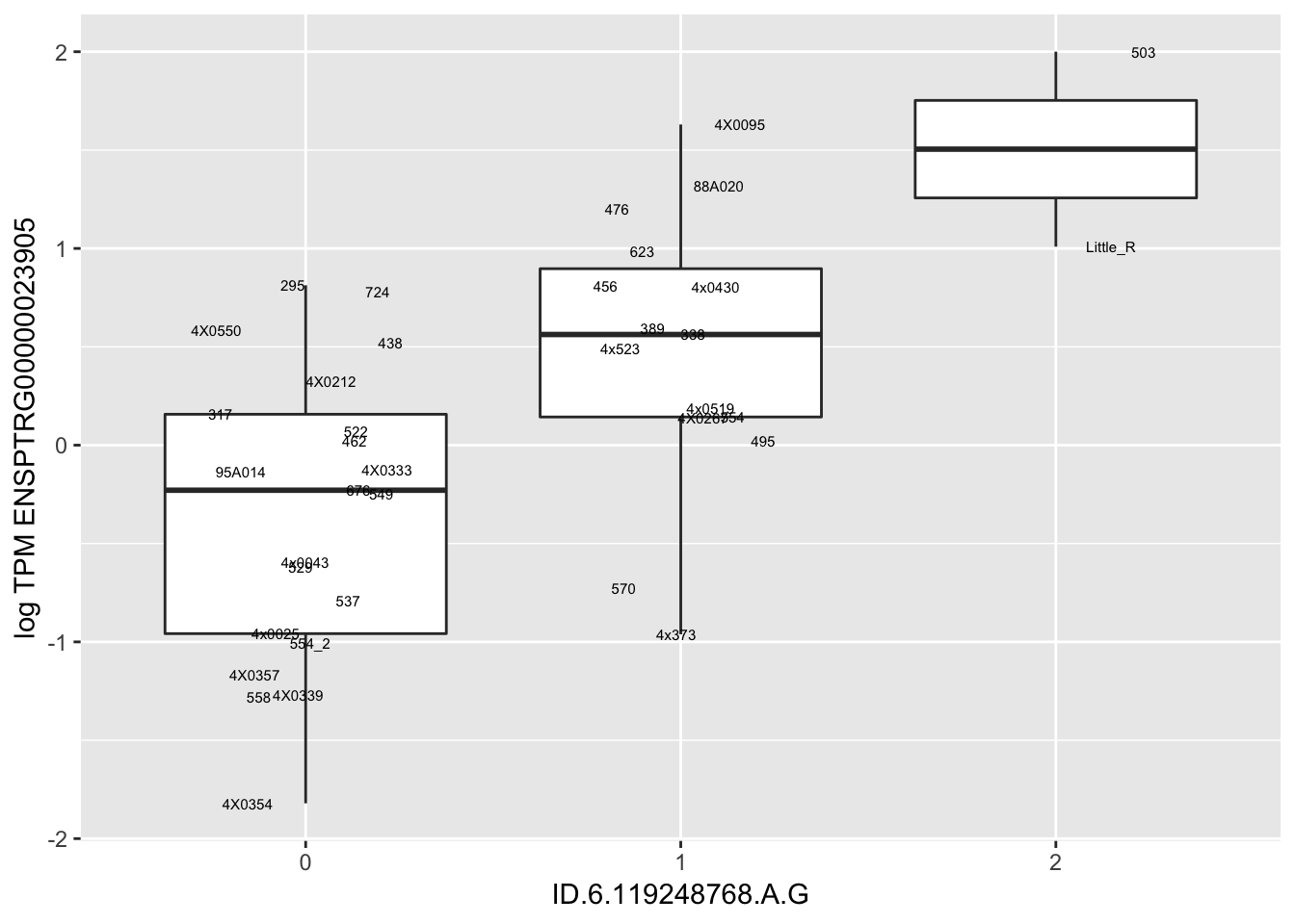
Association testing was implemented in the R package ‘MatrixEQTL’. This resulted in 0 eSNP-gene pairs at FDR<0.1 (Benjamini Hodgeberg correction). QQ-plots didn’t show any P-value inflation relative to the null. From previous (unshown) tests, this lack of significant tests is likely due to the quantile normalizatino step diminishing signal. Even though none of the results are significant after multiple hypothesis correction, I still want to check some of the top nominally significant results to check that they aren’t false positives driven by extreme outliers as I had seen in previous analyses.
# Read in genotypes for eQTLs
Genotypes <- read.table("../data/PastAnalysesDataToKeep/20190428_28_Top5000eqtls.genotypes.raw", header=T, check.names = F, stringsAsFactors = F)
colnames(Genotypes) <- sub("_.*", "", colnames(Genotypes))
# Genotypes[!duplicated(as.list(Genotypes))]
kable(Genotypes[1:10,1:10])| FID | IID | PAT | MAT | SEX | PHENOTYPE | ID.1.569995.A.C | ID.1.572334.G.A | ID.1.572938.G.A | ID.1.573420.T.C |
|---|---|---|---|---|---|---|---|---|---|
| 295 | Pan_troglodytes_ThisStudy | 0 | 0 | 0 | 0.0942329 | 1 | 1 | 1 | 1 |
| 317 | Pan_troglodytes_ThisStudy | 0 | 0 | 0 | -0.1636370 | 0 | 0 | 0 | 0 |
| 338 | Pan_troglodytes_ThisStudy | 0 | 0 | 0 | 0.9834290 | 2 | 2 | 2 | 2 |
| 389 | Pan_troglodytes_ThisStudy | 0 | 0 | 0 | -0.0489686 | 1 | 1 | 1 | 1 |
| 438 | Pan_troglodytes_ThisStudy | 0 | 0 | 0 | 0.4988640 | 1 | 1 | 1 | 1 |
| 456 | Pan_troglodytes_ThisStudy | 0 | 0 | 0 | 1.3135300 | 1 | 1 | 1 | 1 |
| 462 | Pan_troglodytes_ThisStudy | 0 | 0 | 0 | -0.2912500 | 1 | 1 | 0 | 1 |
| 476 | Pan_troglodytes_ThisStudy | 0 | 0 | 0 | -0.2564910 | 1 | 1 | 1 | 1 |
| 495 | Pan_troglodytes_ThisStudy | 0 | 0 | 0 | 0.2979600 | 0 | 0 | 0 | 0 |
| 4x0025 | Pan_troglodytes_ThisStudy | 0 | 0 | 0 | 0.3792720 | 0 | 0 | 0 | 0 |
#Make sure there aren't duplicate columns
length(colnames(Genotypes))
[1] 4890length(unique(colnames(Genotypes)))[1] 4890# Read in eQTLs from MatrixEQTL output (already filtered for FDR<0.1)
eQTLs <- read.table("../data/PastAnalysesDataToKeep/20190428_Top5000eqtls.txt.gz", header=T)
kable(head(eQTLs))| SNP | gene | beta | t.stat | p.value | FDR |
|---|---|---|---|---|---|
| ID.3.10249149.C.CT | ENSPTRG00000043259 | 2.392096 | 8.108636 | 0e+00 | 0.5704260 |
| ID.19.55922879.C.CT | ENSPTRG00000011430 | 2.573798 | 7.122076 | 1e-07 | 0.7419872 |
| ID.22.4961539.C.A | ENSPTRG00000014048 | 2.366572 | 7.010308 | 1e-07 | 0.7419872 |
| ID.14.76525141.A.G | ENSPTRG00000006649 | -1.965541 | -6.955140 | 1e-07 | 0.7419872 |
| ID.14.76528940.A.C | ENSPTRG00000006649 | -1.965541 | -6.955140 | 1e-07 | 0.7419872 |
| ID.14.76551609.A.T | ENSPTRG00000006649 | -1.965541 | -6.955140 | 1e-07 | 0.7419872 |
# This count table is the log10(TPM); no standardization or quantile normalization
# Read in phenotypes, from count table
CountTable <- read.table('../output/log10TPM.StandardizedAndNormalized.txt', header=T, check.names=FALSE, row.names = 1) %>%
  t() %>%
  as.data.frame() %>%
  rownames_to_column(var = "FID")
kable(CountTable[1:10, 1:10])| FID | ENSPTRG00000000001 | ENSPTRG00000000008 | ENSPTRG00000000009 | ENSPTRG00000000021 | ENSPTRG00000000024 | ENSPTRG00000000025 | ENSPTRG00000000027 | ENSPTRG00000000028 | ENSPTRG00000000029 |
|---|---|---|---|---|---|---|---|---|---|
| 4X0095 | 0.8416212 | 0.7757291 | -1.3483746 | -0.7569059 | 0.8308280 | 0.7997104 | 0.0181772 | 0.1034081 | 0.4249217 |
| 4X0212 | -0.7904331 | 0.5565898 | -0.3429953 | -0.4845533 | -1.6069711 | -1.1851636 | 1.4756654 | -1.3947115 | -0.4301090 |
| 4X0267 | 1.5144345 | 0.6001624 | -0.5080765 | -0.1795951 | 1.1635983 | 1.0160362 | 1.1422363 | 0.7078222 | 0.1528507 |
| 4X0333 | 0.5872556 | -2.2634369 | 1.1377030 | -1.3572402 | 2.0259921 | 1.1025578 | -1.0294431 | 1.4817199 | -0.1381548 |
| 4X0339 | -0.2028427 | 1.3151323 | 1.0684250 | 0.6238155 | 1.9458773 | 0.7643574 | 1.0639476 | 1.7375314 | 0.4234417 |
| 4X0354 | -0.5092311 | 1.7291771 | 1.3367160 | -0.4889312 | 0.8910849 | -0.9831549 | 0.3301120 | 2.1964366 | 0.4874074 |
| 4X0357 | 0.5824408 | 0.8583642 | 0.4142126 | 0.8329788 | 1.4642099 | -1.0559415 | 0.6700917 | 1.6976258 | 0.4114508 |
| 4X0550 | -0.5291596 | -1.4100801 | -1.1517021 | -1.2756167 | -0.4564110 | -0.1501142 | -0.1518244 | -1.1134913 | 0.0234199 |
| 4x0025 | 0.3792723 | -1.0562368 | -0.6595468 | 0.5377367 | 0.3076960 | 0.4671330 | -0.5623238 | -0.9211644 | 0.5856492 |
| 4x0043 | -0.1078288 | -1.5091332 | 1.4661884 | 0.7925146 | -1.2210758 | -1.5410475 | 0.5159799 | -1.0317436 | 0.8435503 |
MergedData <- left_join(Genotypes, CountTable, by="FID")#eqtls, ordered from most significant at top
kable(head(eQTLs))| SNP | gene | beta | t.stat | p.value | FDR |
|---|---|---|---|---|---|
| ID.3.10249149.C.CT | ENSPTRG00000043259 | 2.392096 | 8.108636 | 0e+00 | 0.5704260 |
| ID.19.55922879.C.CT | ENSPTRG00000011430 | 2.573798 | 7.122076 | 1e-07 | 0.7419872 |
| ID.22.4961539.C.A | ENSPTRG00000014048 | 2.366572 | 7.010308 | 1e-07 | 0.7419872 |
| ID.14.76525141.A.G | ENSPTRG00000006649 | -1.965541 | -6.955140 | 1e-07 | 0.7419872 |
| ID.14.76528940.A.C | ENSPTRG00000006649 | -1.965541 | -6.955140 | 1e-07 | 0.7419872 |
| ID.14.76551609.A.T | ENSPTRG00000006649 | -1.965541 | -6.955140 | 1e-07 | 0.7419872 |
# betas for these
hist(eQTLs$beta, breaks=20)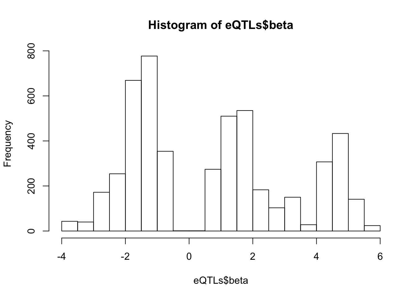 Not sure what to make of that multi-modal distribution of betas (Two peaks around 0 might be expected, but I wasn’t expecting another peak at ~5). Maybe most of these eqtls are the snps in LD that are associated with the same gene…
#how many snps
length(unique(eQTLs$SNP))
[1] 4941#how many genes
length(unique(eQTLs$gene))[1] 1103Average of ~5 snps per gene, so I’m still perplexed by the multiple modes in the distribution of effect sizes.
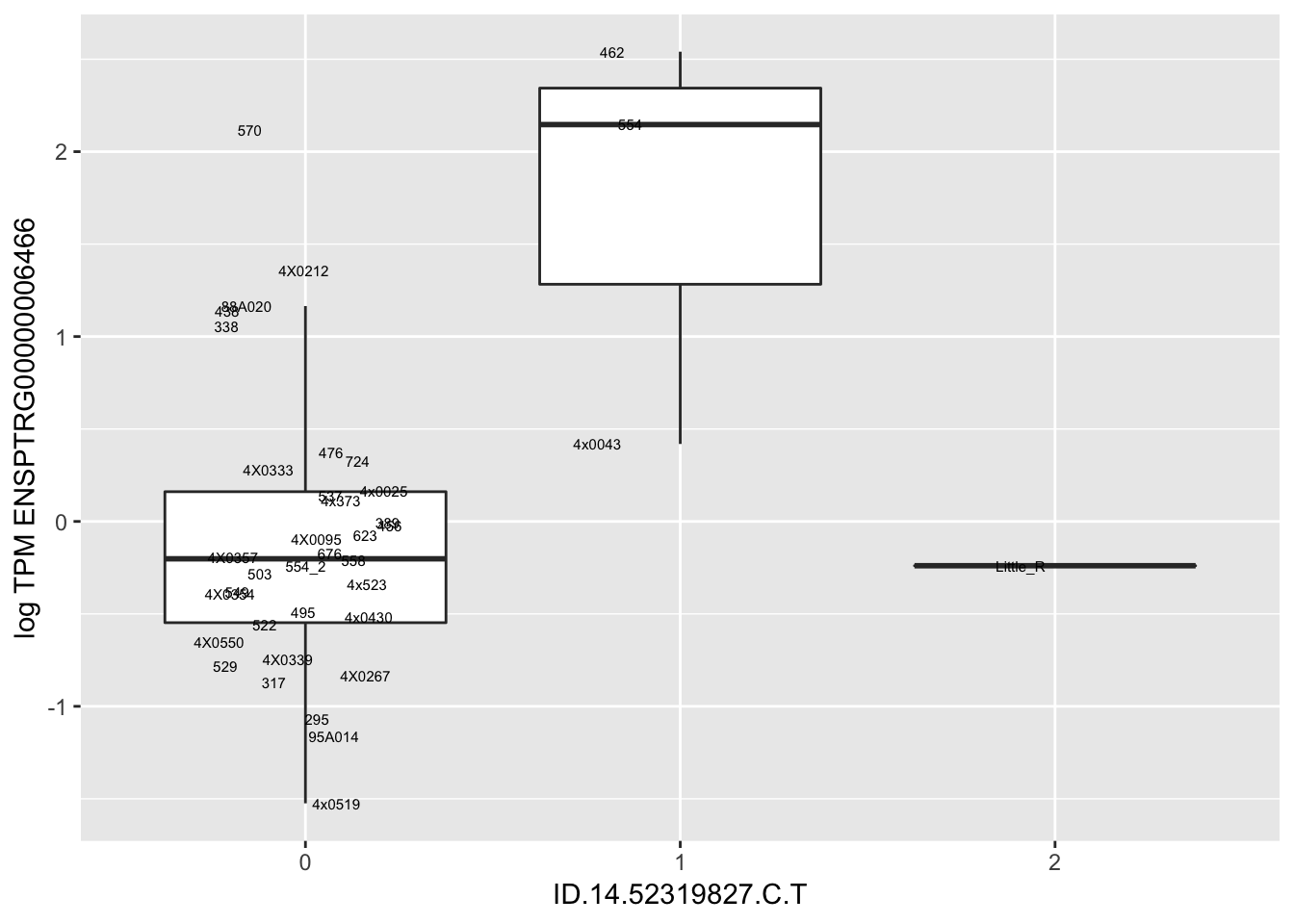
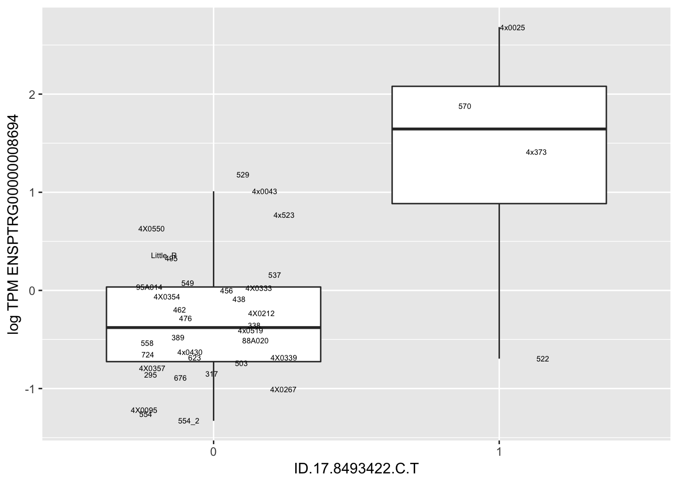
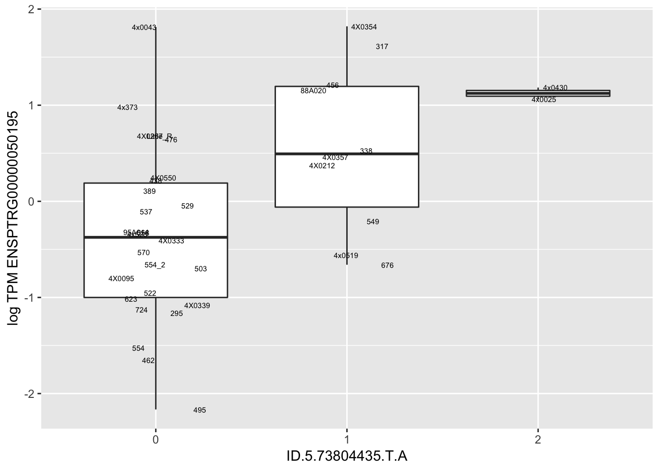
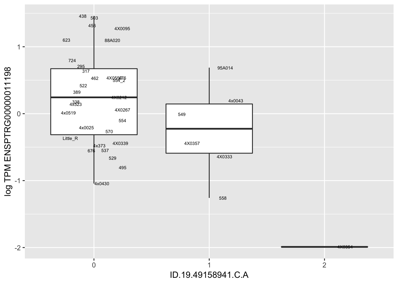
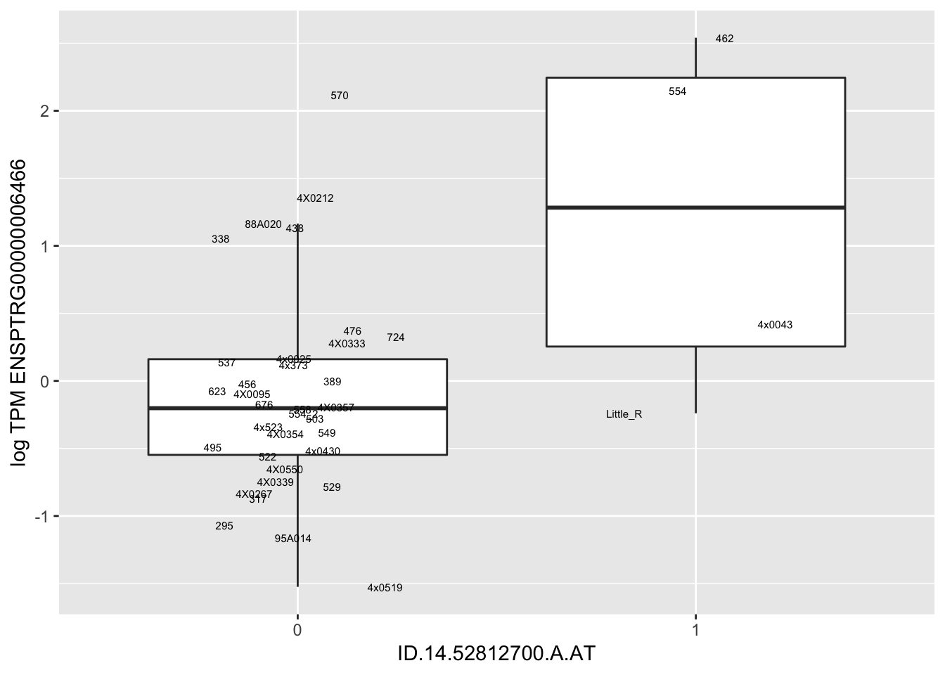
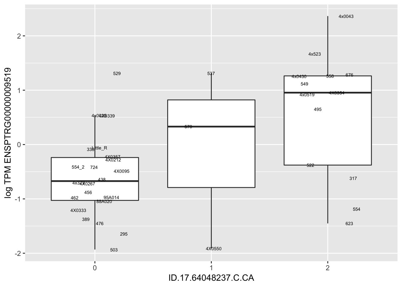
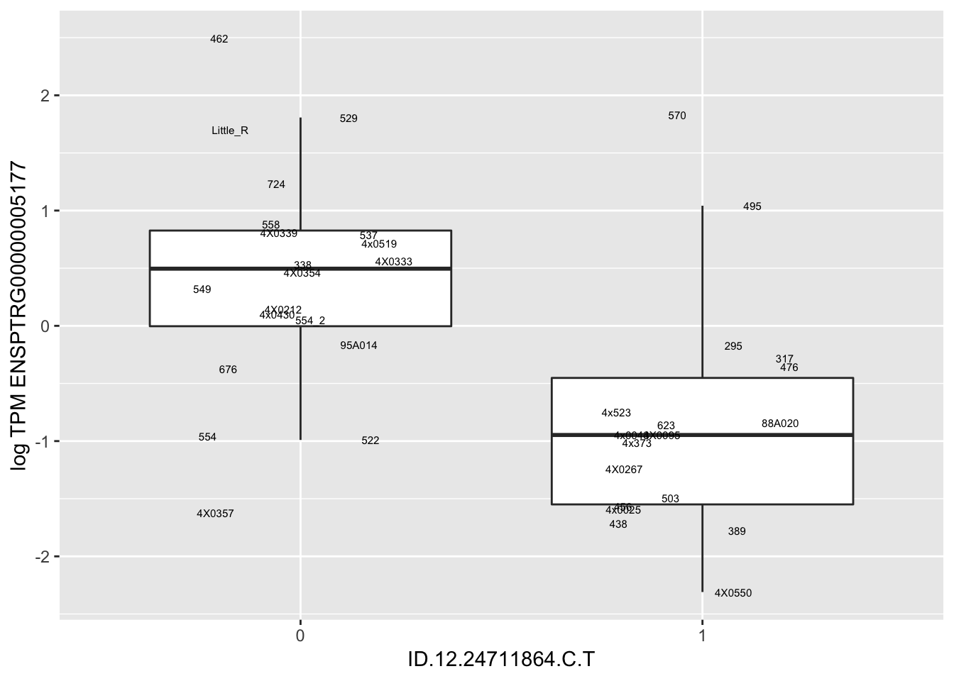
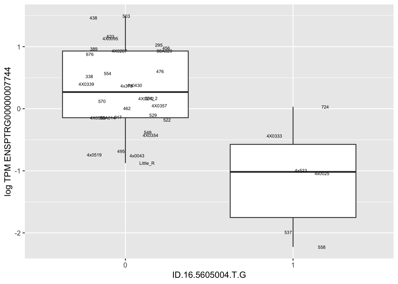
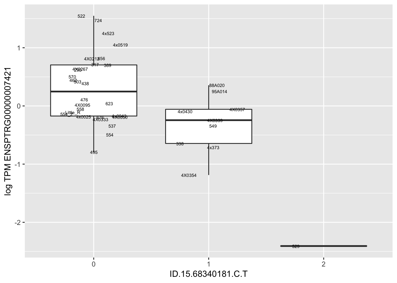
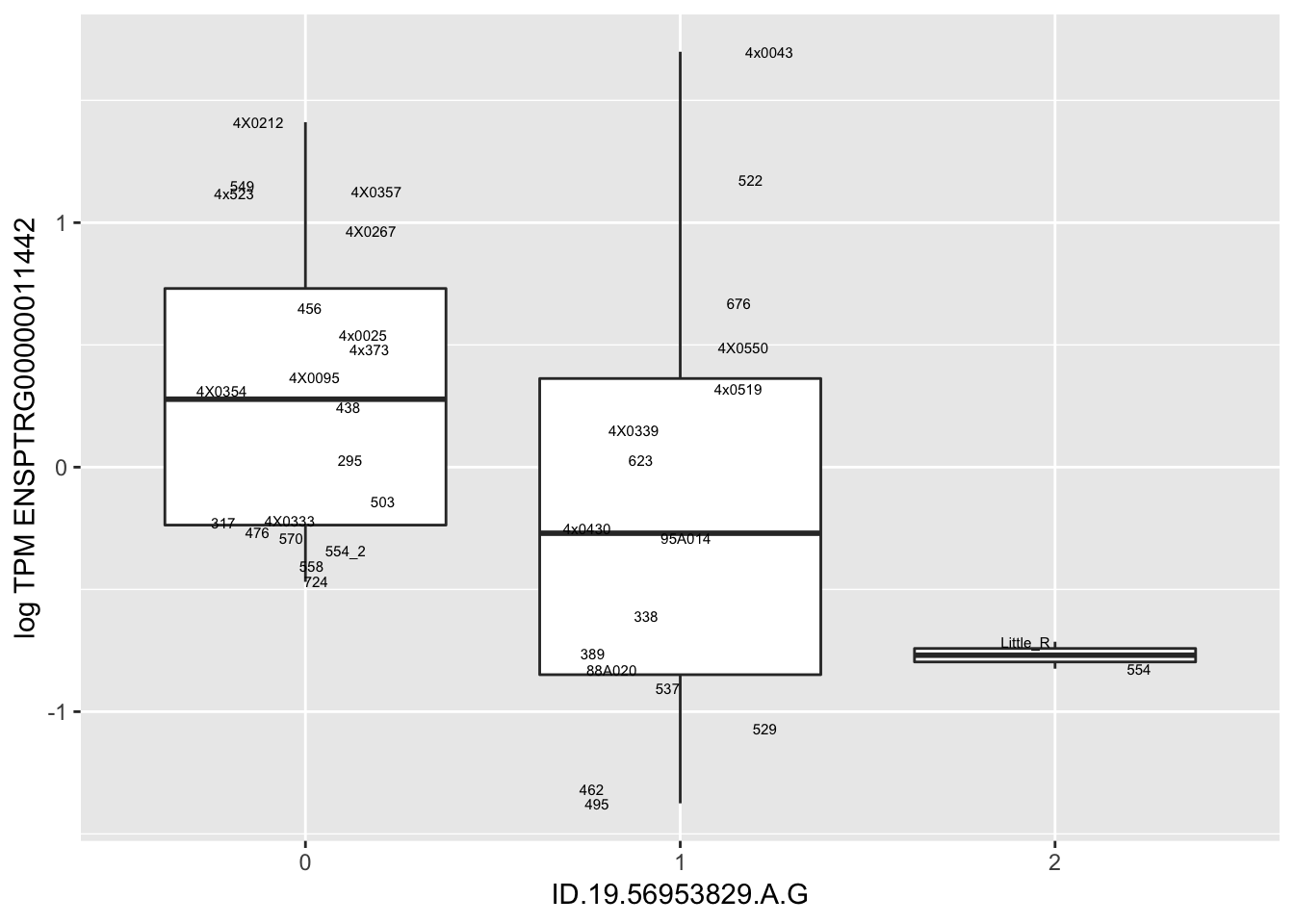
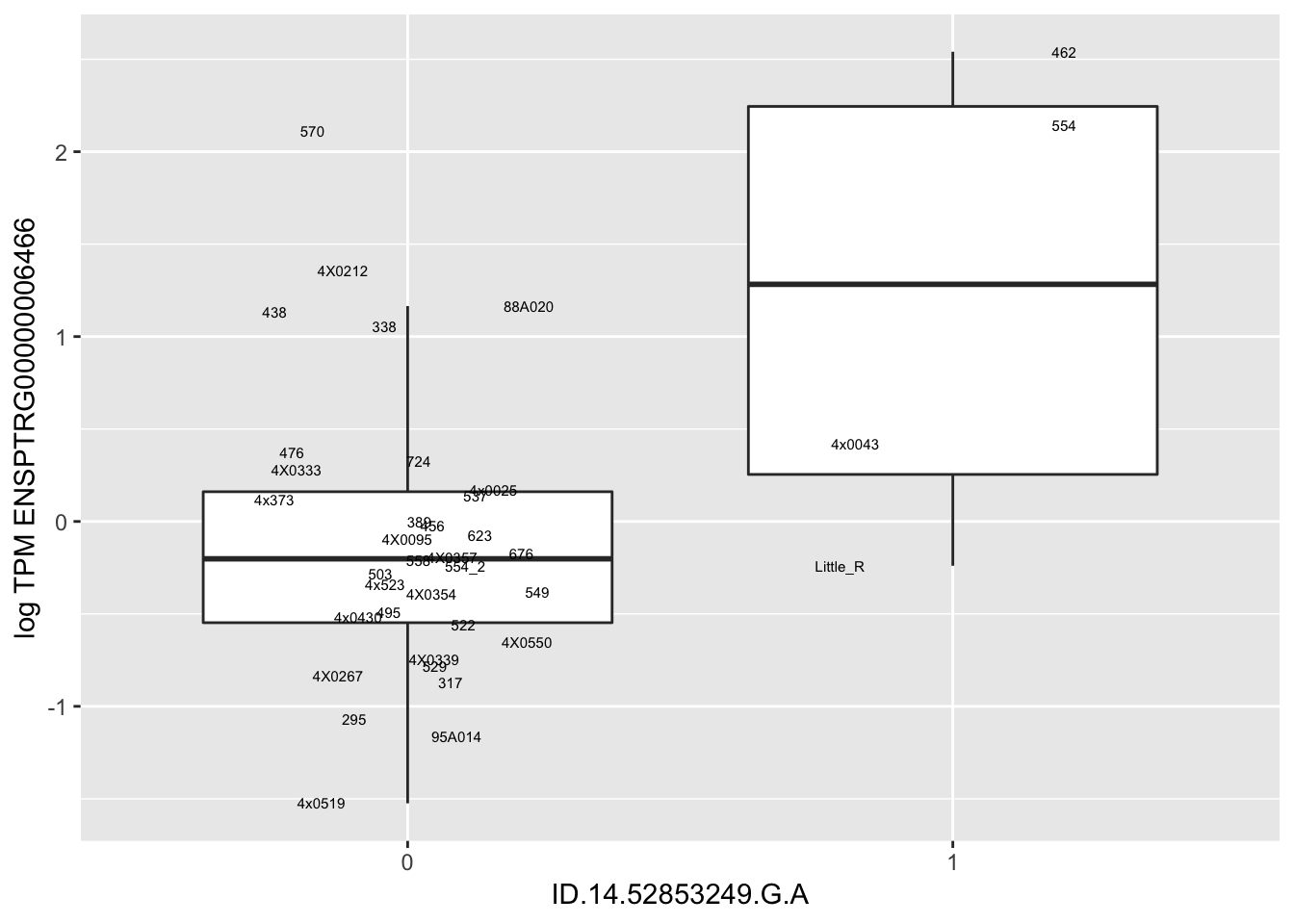
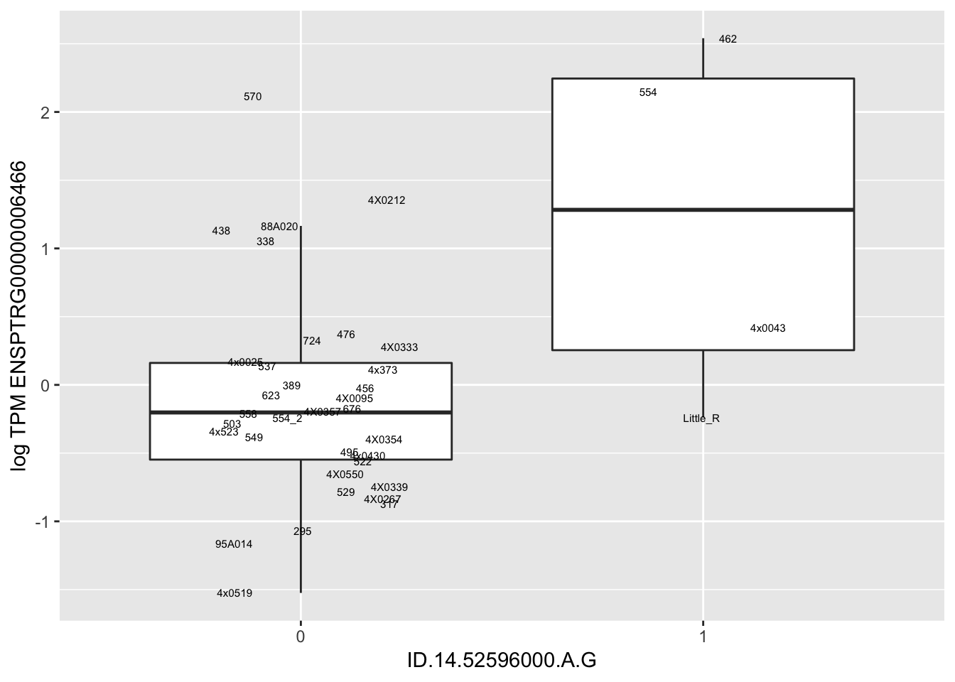
In any case, now I want to check some boxplots
# Expression box plot, stratified by genotype. For a fe of top of the list snp-gene pairs (most significant)
MyBoxplot <- function(DataFrame, Labels.name, SNP.name, Gene.name){
  data.frame(Genotype = DataFrame[[SNP.name]],
    Phenotype = DataFrame[[Gene.name]],
    FID=DataFrame[[Labels.name]]) %>%
    ggplot(aes(x=factor(Genotype), y=Phenotype, label=FID)) +
    geom_boxplot(outlier.shape = NA) +
    geom_text(position=position_jitter(width=0.25), alpha=1, size=2) +
    scale_y_continuous(name=paste("log TPM", Gene.name)) +
    xlab(SNP.name)
}

#Box plot of top3 eqtls
MyBoxplot(MergedData, "FID", "ID.3.10249149.C.CT", "ENSPTRG00000043259")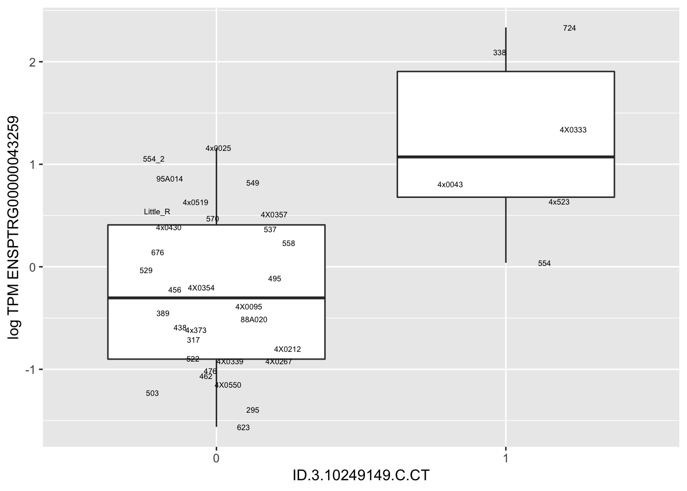
MyBoxplot(MergedData, "FID", "ID.19.55922879.C.CT", "ENSPTRG00000011430")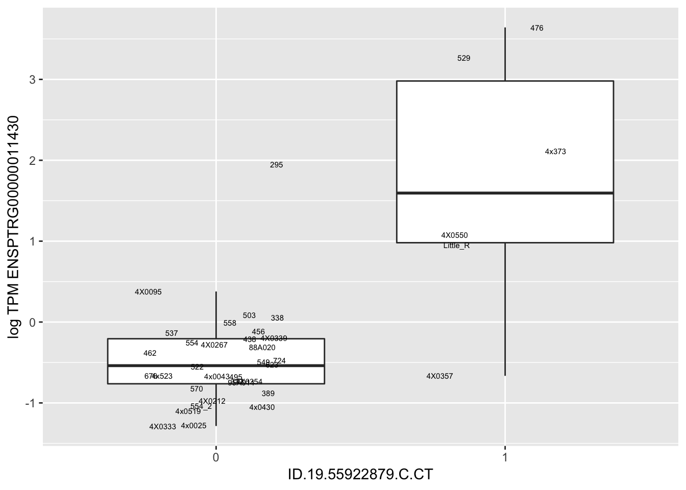
MyBoxplot(MergedData, "FID", "ID.22.4961539.C.A", "ENSPTRG00000014048")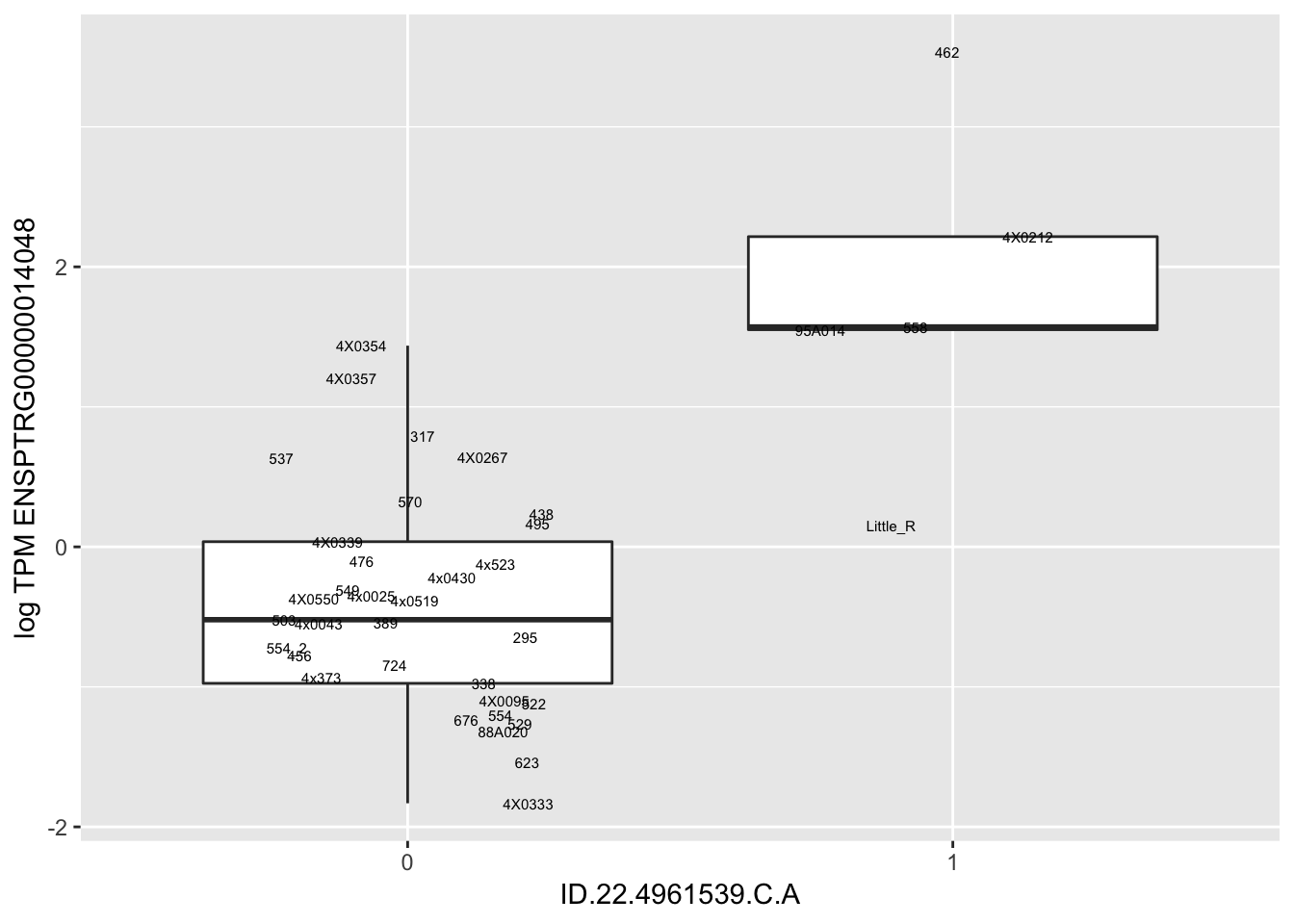 Interpretation: These look more believable than previous analyses without quantile normalization in the sense that these don’t look driven by single outliers. Let’s check some randomly sampled eqtls.
set.seed(1)
RandomSampleOfEqtls <- eQTLs %>% sample_n(20) %>% select(SNP, gene, beta)
kable(RandomSampleOfEqtls)| SNP | gene | beta |
|---|---|---|
| ID.14.52319827.C.T | ENSPTRG00000006466 | 4.4493981 |
| ID.17.8493422.C.T | ENSPTRG00000008694 | 1.7900814 |
| ID.5.73804435.T.A | ENSPTRG00000050195 | 1.2770758 |
| ID.19.49158941.C.A | ENSPTRG00000011198 | -1.1634375 |
| ID.14.52812700.A.AT | ENSPTRG00000006466 | 4.8214705 |
| ID.17.64048237.C.CA | ENSPTRG00000009519 | 0.8118323 |
| ID.12.24711864.C.T | ENSPTRG00000005177 | -1.8386880 |
| ID.16.5605004.T.G | ENSPTRG00000007744 | -1.5800232 |
| ID.15.68340181.C.T | ENSPTRG00000007421 | -1.1271545 |
| ID.19.56953829.A.G | ENSPTRG00000011442 | -1.3466103 |
| ID.14.52853249.G.A | ENSPTRG00000006466 | 4.8214705 |
| ID.14.52596000.A.G | ENSPTRG00000006466 | 4.8214705 |
| ID.5.181283787.G.C | ENSPTRG00000017621 | 1.0340098 |
| ID.12.66200553.G.A | ENSPTRG00000042785 | -0.9109811 |
| ID.1.111084301.A.G | ENSPTRG00000045999 | 2.9252377 |
| ID.14.15972054.A.G | ENSPTRG00000006245 | -1.0287083 |
| ID.15.62588323.C.T | ENSPTRG00000007374 | 0.6043537 |
| ID.12.71441957.T.C | ENSPTRG00000005208 | 4.4265817 |
| ID.22.28305428.G.A | ENSPTRG00000014428 | -1.7638515 |
| ID.6.119248768.A.G | ENSPTRG00000023905 | 1.1430873 |
for(i in 1:nrow(RandomSampleOfEqtls)) {
  try(
    print(MyBoxplot(MergedData, "FID", as.character(RandomSampleOfEqtls$SNP[i]), as.character(RandomSampleOfEqtls$gene[i])))
  )
}
sessionInfo()R version 3.5.1 (2018-07-02)
Platform: x86_64-apple-darwin15.6.0 (64-bit)
Running under: macOS 10.14
Matrix products: default
BLAS: /Library/Frameworks/R.framework/Versions/3.5/Resources/lib/libRblas.0.dylib
LAPACK: /Library/Frameworks/R.framework/Versions/3.5/Resources/lib/libRlapack.dylib
locale:
[1] en_US.UTF-8/en_US.UTF-8/en_US.UTF-8/C/en_US.UTF-8/en_US.UTF-8
attached base packages:
[1] stats graphics grDevices utils datasets methods base
other attached packages:
[1] data.table_1.12.0 knitr_1.22 forcats_0.4.0
[4] stringr_1.4.0 dplyr_0.8.0.1 purrr_0.3.2
[7] readr_1.3.1 tidyr_0.8.2 tibble_2.1.1
[10] ggplot2_3.1.0 tidyverse_1.2.1
loaded via a namespace (and not attached):
[1] Rcpp_1.0.1 highr_0.8 cellranger_1.1.0 plyr_1.8.4
[5] pillar_1.3.1 compiler_3.5.1 git2r_0.24.0 workflowr_1.2.0
[9] tools_3.5.1 digest_0.6.18 lubridate_1.7.4 jsonlite_1.6
[13] evaluate_0.13 nlme_3.1-137 gtable_0.3.0 lattice_0.20-38
[17] pkgconfig_2.0.2 rlang_0.3.3 cli_1.1.0 rstudioapi_0.10
[21] yaml_2.2.0 haven_2.1.0 xfun_0.6 withr_2.1.2
[25] xml2_1.2.0 httr_1.4.0 hms_0.4.2 generics_0.0.2
[29] fs_1.2.6 rprojroot_1.3-2 grid_3.5.1 tidyselect_0.2.5
[33] glue_1.3.1 R6_2.4.0 readxl_1.1.0 rmarkdown_1.11
[37] modelr_0.1.4 magrittr_1.5 whisker_0.3-2 backports_1.1.3
[41] scales_1.0.0 htmltools_0.3.6 rvest_0.3.2 assertthat_0.2.1
[45] colorspace_1.4-1 labeling_0.3 stringi_1.4.3 lazyeval_0.2.2
[49] munsell_0.5.0 broom_0.5.1 crayon_1.3.4