2023-11-02_3MoleculesOfInterestLeafcutterDs
2023-11-02
Last updated: 2023-11-02
Checks: 6 1
Knit directory:
20211209_JingxinRNAseq/analysis/
This reproducible R Markdown analysis was created with workflowr (version 1.7.0). The Checks tab describes the reproducibility checks that were applied when the results were created. The Past versions tab lists the development history.
The R Markdown is untracked by Git. To know which version of the R
Markdown file created these results, you’ll want to first commit it to
the Git repo. If you’re still working on the analysis, you can ignore
this warning. When you’re finished, you can run
wflow_publish to commit the R Markdown file and build the
HTML.
Great job! The global environment was empty. Objects defined in the global environment can affect the analysis in your R Markdown file in unknown ways. For reproduciblity it’s best to always run the code in an empty environment.
The command set.seed(19900924) was run prior to running
the code in the R Markdown file. Setting a seed ensures that any results
that rely on randomness, e.g. subsampling or permutations, are
reproducible.
Great job! Recording the operating system, R version, and package versions is critical for reproducibility.
Nice! There were no cached chunks for this analysis, so you can be confident that you successfully produced the results during this run.
Great job! Using relative paths to the files within your workflowr project makes it easier to run your code on other machines.
Great! You are using Git for version control. Tracking code development and connecting the code version to the results is critical for reproducibility.
The results in this page were generated with repository version 3c2aa40. See the Past versions tab to see a history of the changes made to the R Markdown and HTML files.
Note that you need to be careful to ensure that all relevant files for
the analysis have been committed to Git prior to generating the results
(you can use wflow_publish or
wflow_git_commit). workflowr only checks the R Markdown
file, but you know if there are other scripts or data files that it
depends on. Below is the status of the Git repository when the results
were generated:
Ignored files:
    Ignored:    .DS_Store
    Ignored:    .Rhistory
    Ignored:    .Rproj.user/
    Ignored:    analysis/.RData
    Ignored:    analysis/.Rhistory
    Ignored:    analysis/20220707_TitrationSeries_DE_testing.nb.html
    Ignored:    code/.DS_Store
    Ignored:    code/._DOCK7.pdf
    Ignored:    code/._DOCK7_DMSO1.pdf
    Ignored:    code/._DOCK7_SM2_1.pdf
    Ignored:    code/._FKTN_DMSO_1.pdf
    Ignored:    code/._FKTN_SM2_1.pdf
    Ignored:    code/._MAPT.pdf
    Ignored:    code/._PKD1_DMSO_1.pdf
    Ignored:    code/._PKD1_SM2_1.pdf
    Ignored:    code/.snakemake/
    Ignored:    code/1KG_HighCoverageCalls.samplelist.txt
    Ignored:    code/5ssSeqs.tab
    Ignored:    code/Alignments/
    Ignored:    code/Branaplam_Risdiplam_specific_introns.bed.gz
    Ignored:    code/Branaplam_Risdiplam_specific_introns.bed.gz.tbi
    Ignored:    code/ChemCLIP/
    Ignored:    code/ClinVar/
    Ignored:    code/DE_testing/
    Ignored:    code/DE_tests.mat.counts.gz
    Ignored:    code/DE_tests.txt.gz
    Ignored:    code/DataNotToCommit/
    Ignored:    code/DonorMotifSearches/
    Ignored:    code/DoseResponseData/
    Ignored:    code/Fastq/
    Ignored:    code/FastqFastp/
    Ignored:    code/FivePrimeSpliceSites.txt
    Ignored:    code/FragLenths/
    Ignored:    code/Ishigami/
    Ignored:    code/Meme/
    Ignored:    code/Multiqc/
    Ignored:    code/OMIM/
    Ignored:    code/OldBigWigs/
    Ignored:    code/PhyloP/
    Ignored:    code/QC/
    Ignored:    code/ReferenceGenomes/
    Ignored:    code/Rplots.pdf
    Ignored:    code/Session.vim
    Ignored:    code/Session2.vim
    Ignored:    code/SplicingAnalysis/
    Ignored:    code/TracksSession
    Ignored:    code/bigwigs/
    Ignored:    code/featureCounts/
    Ignored:    code/figs/
    Ignored:    code/fimo_out/
    Ignored:    code/geena/
    Ignored:    code/hg38ToMm39.over.chain.gz
    Ignored:    code/igv_session.template.xml
    Ignored:    code/igv_session.xml
    Ignored:    code/log
    Ignored:    code/logs/
    Ignored:    code/rstudio-server.job
    Ignored:    code/rules/.ExpMoleculesOfInterest.smk.swp
    Ignored:    code/scratch/
    Ignored:    code/temp/
    Ignored:    code/test.txt.gz
    Ignored:    code/testPlottingWithMyScript.ForJingxin.sh
    Ignored:    code/testPlottingWithMyScript.ForJingxin2.sh
    Ignored:    code/testPlottingWithMyScript.ForJingxin3.sh
    Ignored:    code/testPlottingWithMyScript.ForJingxin4.sh
    Ignored:    code/testPlottingWithMyScript.sh
    Ignored:    code/tracks.with_chRNA.RisdiBrana.xml
    Ignored:    code/tracks.with_chRNA.RisdiBranaWithExtras.xml
    Ignored:    code/tracks.xml
    Ignored:    data/~$52CompoundsTempPlateLayoutForPipettingConvenience.xlsx

Untracked files:
    Untracked:  analysis/2023-11-02_3MoleculesOfInterestLeafcutterDs.Rmd
    Untracked:  code/config/samples.3MoleculesOfInterestExperiment.Contrasts.tsv
    Untracked:  code/scripts/Exp202310_MakeLeafcutterContrasts.R

Unstaged changes:
    Modified:   analysis/2023-10-31_Explore3MoleculesOfInterest.Rmd
    Modified:   code/rules/ExpMoleculesOfInterest.smk
    Modified:   code/rules/common.smk
    Modified:   code/scripts/GenometracksByGenotype
Note that any generated files, e.g. HTML, png, CSS, etc., are not included in this status report because it is ok for generated content to have uncommitted changes.
There are no past versions. Publish this analysis with
wflow_publish() to start tracking its development.
Intro
I’ve processed each of three doses for each of three molecules as a leafcutter contrast with 5 DMSO samples… Previously in the firboblast experiment, I noticed a correlation between effect size and different types of NN in NNGA|GT introns… I will similarly look for that here with these three new molecules.
Analysis
load libs
library(tidyverse)
library(RColorBrewer)
library(data.table)
library(gplots)
library(ggrepel)

# define some useful funcs
sample_n_of <- function(data, size, ...) {
  dots <- quos(...)

  group_ids <- data %>%
    group_by(!!! dots) %>%
    group_indices()

  sampled_groups <- sample(unique(group_ids), size)

  data %>%
    filter(group_ids %in% sampled_groups)
}


# Set theme
theme_set(
  theme_classic() +
  theme(text=element_text(size=16,  family="Helvetica")))

# I use layer a lot, to rotate long x-axis labels
Rotate_x_labels <- theme(axis.text.x = element_text(angle = 45, vjust = 1, hjust=1))
Read in data
juncs <- fread("../code/SplicingAnalysis/FullSpliceSiteAnnotations/JuncfilesMerged.annotated.basic.bed.gz") %>%
  mutate(Junc = paste(chrom, start, end, strand, sep="_"))
donors <- fread("../code/SplicingAnalysis/FullSpliceSiteAnnotations/JuncfilesMerged.annotated.basic.bed.5ss.tab.gz", col.names = c("Junc.Donor", "seq", "DonorScore")) %>%
  separate(Junc.Donor, into=c("Junc", "Donor"), sep="::")

Cluster_sig <-
  Sys.glob("../code/SplicingAnalysis/Exp202310_3Molecules_Contrasts/*_cluster_significance.txt") %>%
  setNames(str_replace(., "../code/SplicingAnalysis/Exp202310_3Molecules_Contrasts/(.+?)_cluster_significance.txt", "\\1")) %>%
  append(
    Sys.glob("../code/SplicingAnalysis/leafcutter/differential_splicing/*_cluster_significance.txt") %>%
      grep("ExpOf52", ., invert=T, value=T) %>%
      setNames(str_replace(., "../code/SplicingAnalysis/leafcutter/differential_splicing/(.+?)_cluster_significance.txt", "\\1"))
  ) %>%
  lapply(fread) %>%
  bind_rows(.id="Contrast")

effect_sizes <- Sys.glob("../code/SplicingAnalysis/Exp202310_3Molecules_Contrasts/*_effect_sizes.txt") %>%
  setNames(str_replace(., "../code/SplicingAnalysis/Exp202310_3Molecules_Contrasts/(.+?)_effect_sizes.txt", "\\1")) %>%
  append(
    Sys.glob("../code/SplicingAnalysis/leafcutter/differential_splicing/*_effect_sizes.txt") %>%
      grep("ExpOf52", ., invert=T, value=T) %>%
      setNames(str_replace(., "../code/SplicingAnalysis/leafcutter/differential_splicing/(.+?)_effect_sizes.txt", "\\1"))
  ) %>%
  lapply(fread, col.names=c("intron", "logef", "DMSO", "treatment", "deltapsi")) %>%
  bind_rows(.id="Contrast") %>%
  mutate(Junc = str_replace(intron, "^(.+?):(.+?):(.+?):clu_.+?_([+-])$", "\\1_\\2_\\3_\\4")) %>%
  mutate(cluster = str_replace(intron, "^(.+?):.+?:.+?:(clu_.+?_[+-])$", "\\1:\\2")) %>%
  inner_join(
    inner_join(juncs, donors)
  ) %>%
  inner_join(Cluster_sig) %>%
  mutate(CellType = if_else(str_detect(Contrast, "_"), "LCL", "Fibroblast")) %>%
  mutate(logef = if_else(CellType=="Fibroblast", -1*logef, logef)) %>%
  mutate(logef = if_else(CellType=="Fibroblast", -1*deltapsi, deltapsi)) %>%
  mutate(NN__GU = str_extract(seq, "^\\w{2}")) %>%
  mutate(NNGU = substr(seq, 3, 4))
effect_sizes %>%
filter(p.adjust < 0.01) %>%
ggplot(aes(x=logef, color=Contrast)) +
stat_ecdf() +
geom_vline(xintercept = 0, linetype="dashed") +
geom_vline(
data = . %>%
group_by(NNGU, Contrast) %>%
summarise(med=median(logef, na.rm=T)),
aes(xintercept=med, color=Contrast),
linetype='dashed'
) +
coord_cartesian(xlim=c(-0.5, 0.5)) +
ylab("CumulativeFraction") +
facet_wrap(~NNGU) +
theme_light() +
ggtitle("Effect sizes for NN|GT introns, grouped by NN") +
labs(caption="Only included introns in FDR<0.01 significant clusters")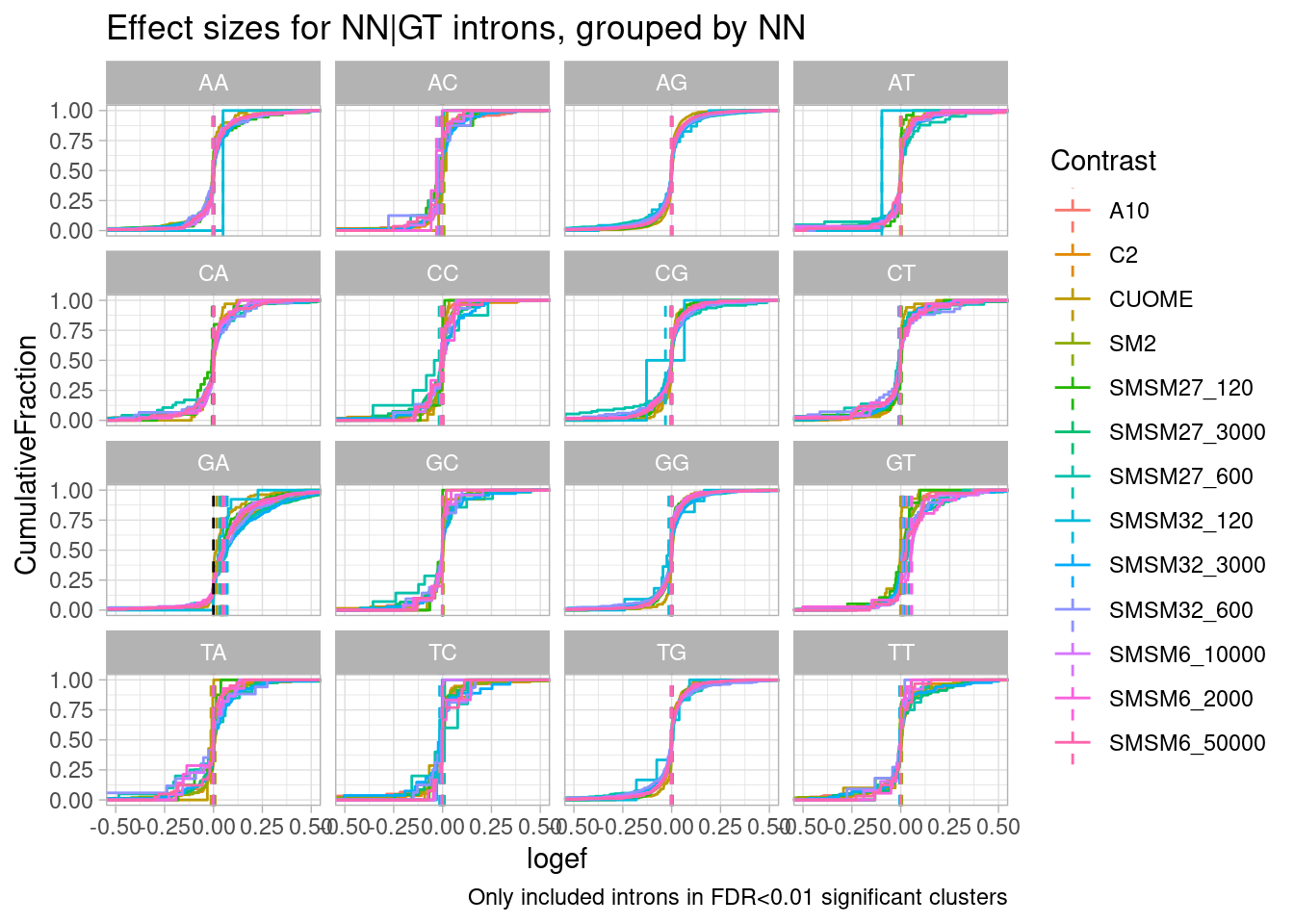
effect_sizes %>%
  # filter(p.adjust < 0.01) %>%
  filter(NNGU=="GA") %>%
  ggplot(aes(x=logef, color=Contrast)) +
  stat_ecdf() +
  geom_vline(xintercept = 0, linetype="dashed") +
  geom_vline(
    data = . %>%
      group_by(NN__GU, Contrast) %>%
      summarise(med=median(logef, na.rm=T)),
    aes(xintercept=med, color=Contrast),
    linetype='dashed'
  ) +
  coord_cartesian(xlim=c(-0.5, 0.5)) +
  ylab("CumulativeFraction") +
  facet_wrap(~NN__GU) +
  theme_light() +
  ggtitle("Effect sizes for NNGA|GT introns, grouped by NN") +
  labs(caption="All tested GA|GU")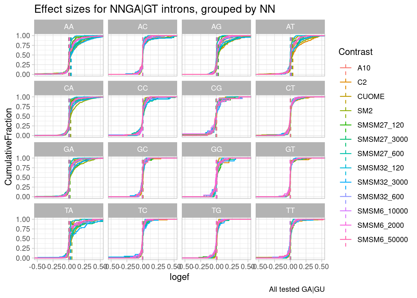
Make same plot with less samples… There’s a lot of clutter…
Colors <- effect_sizes %>%
  distinct(Contrast) %>%
  mutate(Colors = recode(Contrast, SMSM27_3000="#3182bd", SMSM27_600="#9ecae1", SMSM27_120="#deebf7", SMSM32_120="#fee0d2", SMSM32_3000="#de2d26", SMSM32_600="#fc9272", SMSM6_10000="#a65628", SMSM6_2000="#a65628", SMSM6_50000="#a65628", A10="#7fc97f", C2="#beaed4", CUOME="#fdc086", SM2="#ffff99")) %>%
  dplyr::select(Contrast, Colors) %>% deframe()

Colors.Subset <- effect_sizes %>%
  distinct(Contrast) %>%
  filter(Contrast %in% c("SM2", "C2", "SMSM27_3000", "SMSM27_600", "SMSM32_3000", "SMSM32_600", "SMSM6_50000")) %>%
  mutate(Colors = recode(Contrast, SMSM6_50000="#b15928", SMSM27_3000="#e31a1c", SMSM27_600="#fb9a99", SMSM32_3000="#ff7f00", SMSM32_600="#fdbf6f", C2="#377eb8", SM2="#4daf4a")) %>%
  dplyr::select(Contrast, Colors) %>% deframe()

effect_sizes %>%
  # filter(p.adjust < 0.01) %>%
  filter(Contrast %in% names(Colors.Subset)) %>%
  filter(NNGU=="GA") %>%
  group_by(NN__GU) %>%
  mutate(Unique_Elements = n_distinct(intron)) %>%   # Now summarise with unique elements per group
  ungroup() %>%
  mutate(FacetGroup = str_glue("{NN__GU}; n={Unique_Elements}")) %>%
  ggplot(aes(x=logef, color=Contrast)) +
  stat_ecdf() +
  geom_vline(xintercept = 0, linetype="dashed") +
  geom_vline(
    data = . %>%
      group_by(FacetGroup, Contrast) %>%
      summarise(med=median(logef, na.rm=T)),
    aes(xintercept=med, color=Contrast),
    linetype='dashed'
  ) +
  scale_color_manual(values=Colors.Subset, drop=T) +
  coord_cartesian(xlim=c(-0.1, 0.1)) +
  ylab("CumulativeFraction") +
  facet_wrap(~FacetGroup) +
  theme_light() +
  ggtitle("Effect sizes for NNGA|GT introns, grouped by NN") +
  labs(caption="All leafcutter-tested GA|GU")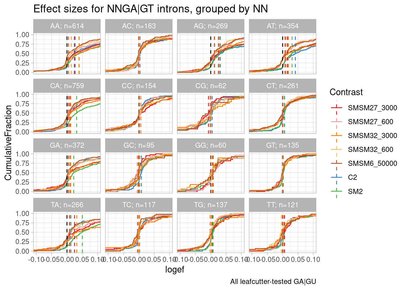
So first recall this plot I have made in the past, where the x-axis is the spearman dose:PSI correlation coefficient, sort of a proxy for effects on different NN sub-categories of NNGA|GU introns. branaplam has stronger effects on GA, CA, and TA… but AA looks more or less the same between risdiplam/branaplam… AT maybe looks a bit risdiplam specific… This btw is the same sequence in that risdiplam-specific sequence in HSD17B4 which has two poison exons. In any case, now look at the second plot, where the x-axis is the logef (from leafcutter) for introns with these different groups… I also included some data from the fibroblast experiment: SM2 (colored green, because it is a branaplam scaffold) and C2 (colored blue because it is a risdiplam scaffold). Again just looking at SM2 and C2, the relative effects between classes are mostly consistent with the dose titration experiment with risdiplam and branaplam… Anyway, now looking at SMSM27 and SMSM32 (the red and orange), the effects look stronger than C2 for the GA and CA facets… Again, its tricky to compare, because the effective genome-wide dose isn’t exactly the same between experiments, and the cell type is different… But I figure that by looking across different facets you can sort of control for those things. So from that, I do feel in some ways these molecules do have some slight branaplam-like-character moreso than risdiplam.
sessionInfo()R version 4.2.0 (2022-04-22)
Platform: x86_64-pc-linux-gnu (64-bit)
Running under: CentOS Linux 7 (Core)
Matrix products: default
BLAS/LAPACK: /software/openblas-0.3.13-el7-x86_64/lib/libopenblas_haswellp-r0.3.13.so
locale:
[1] LC_CTYPE=en_US.UTF-8 LC_NUMERIC=C LC_TIME=C
[4] LC_COLLATE=C LC_MONETARY=C LC_MESSAGES=C
[7] LC_PAPER=C LC_NAME=C LC_ADDRESS=C
[10] LC_TELEPHONE=C LC_MEASUREMENT=C LC_IDENTIFICATION=C
attached base packages:
[1] stats graphics grDevices utils datasets methods base
other attached packages:
[1] ggrepel_0.9.1 gplots_3.1.3 data.table_1.14.2 RColorBrewer_1.1-3
[5] forcats_0.5.1 stringr_1.4.0 dplyr_1.0.9 purrr_0.3.4
[9] readr_2.1.2 tidyr_1.2.0 tibble_3.1.7 ggplot2_3.3.6
[13] tidyverse_1.3.1
loaded via a namespace (and not attached):
[1] httr_1.4.3 sass_0.4.1 jsonlite_1.8.0 R.utils_2.11.0
[5] modelr_0.1.8 gtools_3.9.2 bslib_0.3.1 assertthat_0.2.1
[9] highr_0.9 cellranger_1.1.0 yaml_2.3.5 pillar_1.7.0
[13] backports_1.4.1 glue_1.6.2 digest_0.6.29 promises_1.2.0.1
[17] rvest_1.0.2 colorspace_2.0-3 htmltools_0.5.2 httpuv_1.6.5
[21] R.oo_1.24.0 pkgconfig_2.0.3 broom_0.8.0 haven_2.5.0
[25] scales_1.2.0 later_1.3.0 tzdb_0.3.0 git2r_0.30.1
[29] generics_0.1.2 farver_2.1.0 ellipsis_0.3.2 withr_2.5.0
[33] cli_3.3.0 magrittr_2.0.3 crayon_1.5.1 readxl_1.4.0
[37] evaluate_0.15 R.methodsS3_1.8.1 fs_1.5.2 fansi_1.0.3
[41] xml2_1.3.3 tools_4.2.0 hms_1.1.1 lifecycle_1.0.1
[45] munsell_0.5.0 reprex_2.0.1 compiler_4.2.0 jquerylib_0.1.4
[49] caTools_1.18.2 rlang_1.0.2 grid_4.2.0 rstudioapi_0.13
[53] bitops_1.0-7 labeling_0.4.2 rmarkdown_2.14 gtable_0.3.0
[57] DBI_1.1.2 R6_2.5.1 lubridate_1.8.0 knitr_1.39
[61] fastmap_1.1.0 utf8_1.2.2 workflowr_1.7.0 rprojroot_2.0.3
[65] KernSmooth_2.23-20 stringi_1.7.6 Rcpp_1.0.8.3 vctrs_0.4.1
[69] dbplyr_2.1.1 tidyselect_1.1.2 xfun_0.30