20220712_FitDoseResponseModel

Intro

Here I will fit dose response curves using drc.

• C2-C5-1: 1000, 316, 100, 31.6, 10, 3.16, 1, 0.316 nM
• Branaplam: 3,160, 1000, 316, 100, 31.6, 10, 3.16, 1 nM.
• Risdiplam: 10,000, 3,160, 1000, 316, 100, 31.6, 10, 3.16 nM

Results

First load in libraries

library(tidyverse)
library(edgeR)
library(RColorBrewer)
library(gplots)
library(viridis)
library(broom)
library(qvalue)
library(drc)

library(sandwich)
library(lmtest)

…and read in data, and subset genes with mean expression \(log_2(CountPerMillion)>1\).

dat <- read_tsv("../code/featureCounts/Counts.titration_series.txt", comment="#") %>%
  rename_at(vars(-(1:6)), ~str_replace(.x, "Alignments/STAR_Align/TitrationExp(.+?)/Aligned.sortedByCoord.out.bam", "\\1")) %>%
  dplyr::select(Geneid, everything(), -c(2:6)) %>%
  column_to_rownames("Geneid") %>%
  DGEList()

ColorsTreatments <- c("blue"="Bran", "red"="C2C5", "green"="Ris")

mean.cpm <- dat %>%
    cpm(log=T) %>%
    apply(1, mean)

ExpressedGenes.CPM <- dat[mean.cpm>1,] %>%
  calcNormFactors() %>%
  cpm(prior.count=0.1)

# Read in gene names. Note that ensembl_id to hgnc_symbol is not a 1-to-1 mapping
geneNames <- read_tsv("../data/Genes.list.txt") %>%
  mutate(hgnc_symbol = coalesce(hgnc_symbol,ensembl_gene_id)) %>%
  inner_join(data.frame(ensembl.full=rownames(ExpressedGenes.CPM)) %>%
               mutate(ensembl_gene_id = str_remove(ensembl.full, "\\..+$")),
             by = "ensembl_gene_id"
             ) %>%
  dplyr::select(ensembl.full, hgnc_symbol)

Now I will tidy the data a little bit, adding dose information to each sample. For purposes of model fitting, I will add all three DMSO replicates to each titration series as \(dose=0\), which can be handled by the standard 4 parameter log-logistic model implemented in drc.

dat.long <- ExpressedGenes.CPM %>%
  as.data.frame() %>%
  rownames_to_column("gene") %>%
  gather("sample", "cpm", -gene) %>%
  separate(sample, into=c("Treatment", "TitrationPoint"), remove = F, convert = T)

dat.DMSO <- dat.long %>%
  filter(Treatment == "DMSO") %>%
  mutate(dose.nM = 0) %>%
  bind_rows(., ., ., .id="Treatment") %>%
  mutate(Treatment = case_when(
    Treatment == 1 ~ "Bran",
    Treatment == 2 ~ "Ris",
    Treatment == 3 ~ "C2C5"
  ))


Doses <- data.frame(C2C5=c(1000, 316, 100, 31.6, 10, 3.16, 1, 0.316),
           Bran=c(3160, 1000, 316, 100, 31.6, 10, 3.16, 1),
           Ris=c(10000, 3160, 1000, 316, 100, 31.6, 10, 3.16)) %>%
  mutate(TitrationPoint = 1:8) %>%
  gather(key="Treatment", value="dose.nM", -TitrationPoint)

dat.tidy <- dat.long %>%
  filter(!Treatment == "DMSO") %>%
  inner_join(Doses, by=c("Treatment", "TitrationPoint")) %>%
  bind_rows(dat.DMSO) %>%
  inner_join(geneNames, by=c("gene"="ensembl.full"))


head(dat.tidy)

               gene sample Treatment TitrationPoint        cpm dose.nM
1 ENSG00000227232.5 Bran-1      Bran              1   6.725514    3160
2 ENSG00000279457.4 Bran-1      Bran              1  11.998077    3160
3 ENSG00000225972.1 Bran-1      Bran              1   9.661373    3160
4 ENSG00000225630.1 Bran-1      Bran              1 363.612135    3160
5 ENSG00000237973.1 Bran-1      Bran              1 449.156477    3160
6 ENSG00000229344.1 Bran-1      Bran              1   4.972986    3160
  hgnc_symbol
1      WASH7P
2      WASH9P
3    MTND1P23
4    MTND2P28
5    MTCO1P12
6    MTCO2P12

Now that the data is “tidy”, with one row for each treatment:dose:gene combination, I should be able to easily fit models for each treatment:gene group.

Let’s pick one treatment:gene combination for an illustrative example, and fit the 4 parameter log-logistic model, constraining the upper and lower limit parameters to be position (since CPM cannot be negative).

fitted_curve <- dat.tidy %>%
  filter(hgnc_symbol=="STAT1" & Treatment == "Ris") %>%
  drm(formula = cpm ~ dose.nM,
                    data = .,
                    fct = LL.4(names=c("Steepness", "LowerLimit", "UpperLimit", "ED50")),
      lowerl = c(NA, 0, 0, NA))

plot(fitted_curve, type="all")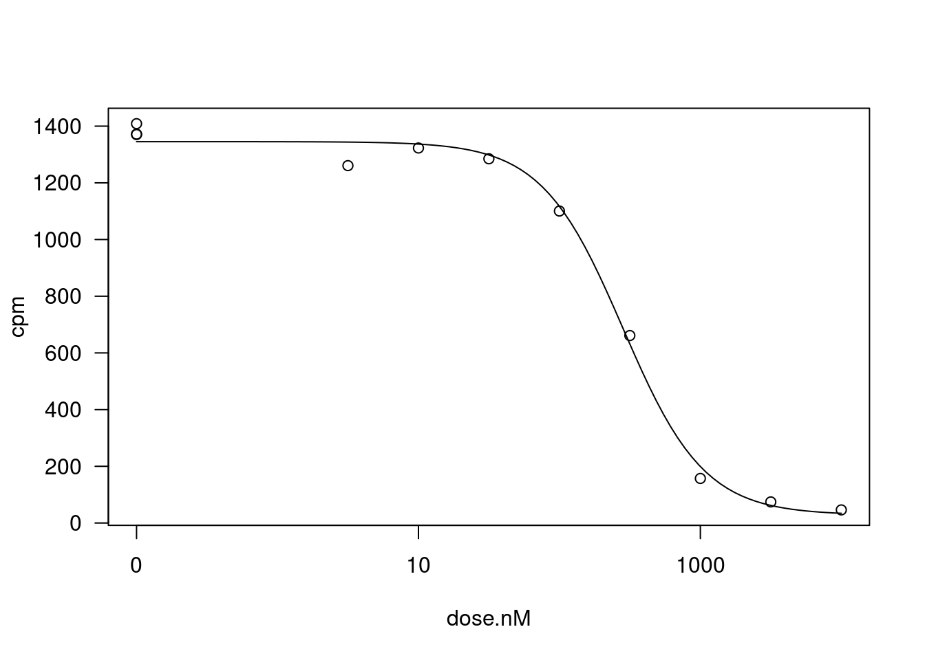

summary(fitted_curve)

Model fitted: Log-logistic (ED50 as parameter) (4 parms)

Parameter estimates:

                         Estimate Std. Error t-value   p-value    
Steepness:(Intercept)     1.50491    0.20358  7.3923 0.0001504 ***
LowerLimit:(Intercept)   28.16274   38.01078  0.7409 0.4828536    
UpperLimit:(Intercept) 1345.21964   21.23941 63.3360 6.425e-11 ***
ED50:(Intercept)        282.55139   27.47342 10.2845 1.778e-05 ***
---
Signif. codes:  0 '***' 0.001 '**' 0.01 '*' 0.05 '.' 0.1 ' ' 1

Residual standard error:

 47.58045 (7 degrees of freedom)

glance(fitted_curve)

# A tibble: 1 × 4
    AIC   BIC logLik    df.residual
  <dbl> <dbl> <logLik>        <int>
1  121.  123. -55.60905           7

According to the drc author’s Plos-one paper supplement, more robust estimates of coefficeint standard errors can be obtained like this:

coeftest(fitted_curve, vcov = sandwich)

t test of coefficients:

                         Estimate Std. Error t value  Pr(>|t|)    
Steepness:(Intercept)     1.50491    0.13151 11.4431 8.741e-06 ***
LowerLimit:(Intercept)   28.16274   11.61893  2.4239   0.04583 *  
UpperLimit:(Intercept) 1345.21964   22.07443 60.9402 8.412e-11 ***
ED50:(Intercept)        282.55139   16.32676 17.3060 5.287e-07 ***
---
Signif. codes:  0 '***' 0.001 '**' 0.01 '*' 0.05 '.' 0.1 ' ' 1

It’s not clear to me whether the response I should be fitting should be \(CPM\) or \(log(CPM)\) for gene expression level. Let’s repeat the process now modelling \(log(CPM)\)

fitted_curve <- dat.tidy %>%
  filter(hgnc_symbol=="STAT1" & Treatment == "Ris") %>%
  drm(formula = log(cpm) ~ dose.nM,
                    data = .,
                    fct = LL.4(names=c("Steepness", "LowerLimit", "UpperLimit", "ED50")),
      lowerl = c())

plot(fitted_curve, type="all")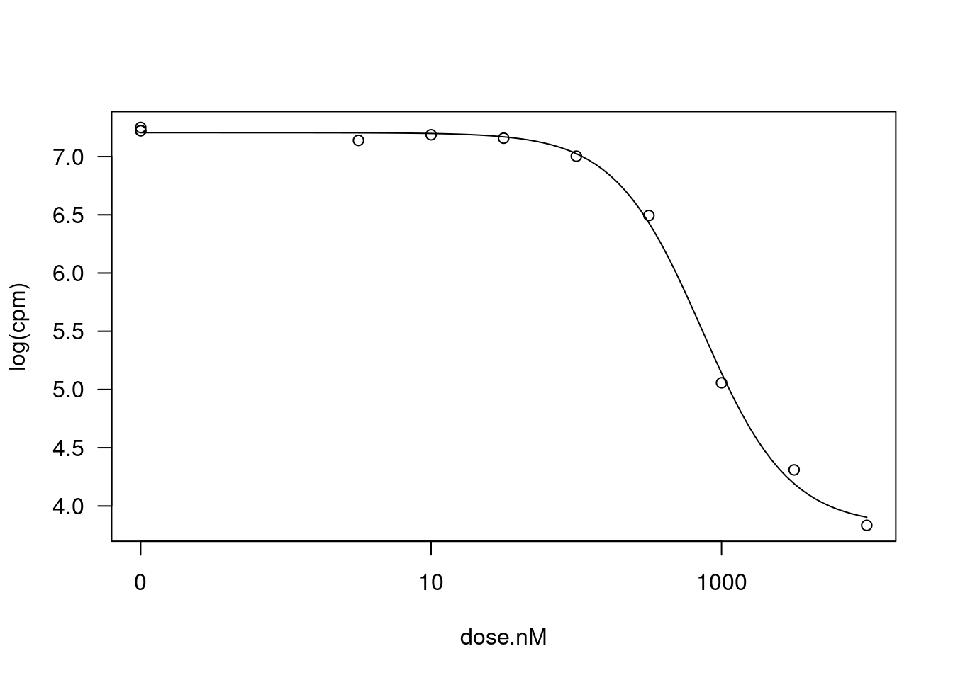

summary(fitted_curve)

Model fitted: Log-logistic (ED50 as parameter) (4 parms)

Parameter estimates:

                         Estimate Std. Error t-value   p-value    
Steepness:(Intercept)    1.446211   0.133727  10.815 1.274e-05 ***
LowerLimit:(Intercept)   3.828167   0.090682  42.215 1.092e-09 ***
UpperLimit:(Intercept)   7.205443   0.030250 238.196 6.143e-15 ***
ED50:(Intercept)       730.890420  53.252969  13.725 2.570e-06 ***
---
Signif. codes:  0 '***' 0.001 '**' 0.01 '*' 0.05 '.' 0.1 ' ' 1

Residual standard error:

 0.0730794 (7 degrees of freedom)

coeftest(fitted_curve, vcov = sandwich)

t test of coefficients:

                         Estimate Std. Error t value  Pr(>|t|)    
Steepness:(Intercept)    1.446211   0.141243  10.239 1.830e-05 ***
LowerLimit:(Intercept)   3.828167   0.094068  40.696 1.410e-09 ***
UpperLimit:(Intercept)   7.205443   0.016000 450.344 < 2.2e-16 ***
ED50:(Intercept)       730.890420  58.873919  12.415 5.061e-06 ***
---
Signif. codes:  0 '***' 0.001 '**' 0.01 '*' 0.05 '.' 0.1 ' ' 1

glance(fitted_curve)

# A tibble: 1 × 4
    AIC   BIC logLik   df.residual
  <dbl> <dbl> <logLik>       <int>
1 -21.3 -19.3 15.65589           7

That also looks like a good fit. Just as a sanity check, let’s compare the AIC between this model, versus a linear model.

# glance at some stats about the log-logistic model fit
glance(fitted_curve)

# A tibble: 1 × 4
    AIC   BIC logLik   df.residual
  <dbl> <dbl> <logLik>       <int>
1 -21.3 -19.3 15.65589           7

#fit an linear model
fitted_curve.lm <- dat.tidy %>%
  filter(hgnc_symbol=="STAT1" & Treatment == "Ris") %>%
  lm(formula = log(cpm) ~ dose.nM,
                    data = .)

# glance at some stats about the log-logistic model fit
glance(fitted_curve.lm)

# A tibble: 1 × 12
  r.squared adj.r.squared sigma statistic p.value    df logLik   AIC   BIC
      <dbl>         <dbl> <dbl>     <dbl>   <dbl> <dbl>  <dbl> <dbl> <dbl>
1     0.693         0.659 0.760      20.3 0.00147     1  -11.5  29.0  30.2
# … with 3 more variables: deviance <dbl>, df.residual <int>, nobs <int>

The log-logistic model is obviously a reasonable fit, and the AIC also shows this log-linear model is a better fit than the simple linear model.

For now I will continue just modelling \(CPM\) (as opposed to \(log(CPM)\)) for simplicity, and at least attempt to fit a log-logistic model for each gene… I can think later about how to prune out the questionable model fits before subsequent analyses. One sort of reasonable way to prune out questionable models I think will be to simply to fit a linear model and only consider gene:treatment combinations where the log-linear fit model is obviously better than the simple linear model (\(\Delta AIC>2\)).

Now let’s try to fit to all gene:treatment combinations…

Actually, to save computation time, at first let’s just try fitting to 100 gene:treatment combinations, and peruse the results.

sample_n_of <- function(data, size, ...) {
  dots <- quos(...)
  
  group_ids <- data %>% 
    group_by(!!! dots) %>% 
    group_indices()
  
  sampled_groups <- sample(unique(group_ids), size)
  
  data %>% 
    filter(group_ids %in% sampled_groups)
}

GenesOfInterest <- c("MAPT", "SNCA", "SMN2", "HTT", "GALC", "FOXM1", "STAT1", "AKT3", "PDGFRB")

# had to use possibly wrapper function to handle errors, like when drm fitting does not converge
safe_drm <- possibly(drm, otherwise=NA)


set.seed(0)
dat.fitted <-
  dat.tidy %>%
  sample_n_of(100, Treatment, gene) %>%
  group_by(Treatment, gene) %>% 
  # filter(hgnc_symbol=="STAT1") %>%
  # filter(hgnc_symbol %in% GenesOfInterest) %>%
  nest(-Treatment, -gene) %>%
  mutate(model = map(data, ~safe_drm(formula = cpm ~ dose.nM,
                    data = .,
                    fct = LL.4(names=c("Steepness", "LowerLimit", "UpperLimit", "ED50"))))) %>%
  # filter out the wrapper functions that returned list with NA
  filter(!anyNA(model))

Error in optim(startVec, opfct, hessian = TRUE, method = optMethod, control = list(maxit = maxIt,  : 
  non-finite finite-difference value [4]

dat.fitted.summarised <- dat.fitted %>%
  mutate(results = map(model, tidy)) %>%
  unnest(results) %>%
  mutate(summary = map(model, glance)) %>%
  unnest(summary)

dat.fitted %>%
  mutate(resid = map(model, residuals)) %>%
  unnest(data, resid) %>%
  ggplot(aes(x=log(cpm), y=resid)) +
  coord_cartesian(xlim=c(0,6), ylim=c(-20,20)) +
  labs(title="Residuals as a function of CPM", caption="modelled CPM; not logCPM") +
  geom_point() +
  theme_bw()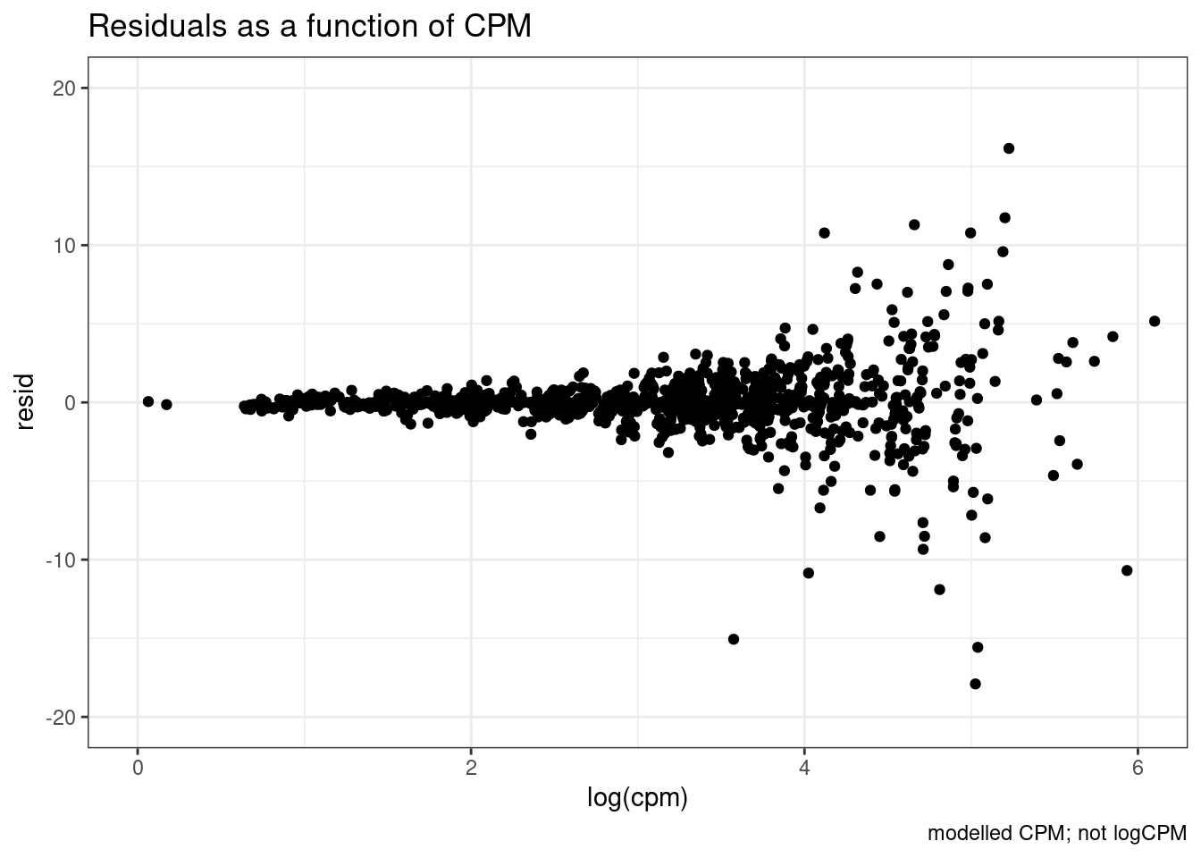

So there is sort of unsurprisingly some heterskedastic errors… More reason to try modelling log(CPM)…

Let’s also check the data for a gene where the model could not be fit: ENSG00000180773.15 with risdiplam.

dat.tidy %>%
  filter(gene == "ENSG00000180773.15") %>%
  ggplot(aes(x=dose.nM, y=cpm, color=Treatment)) +
  geom_point() +
  geom_smooth(method="loess") +
  scale_x_continuous(trans="log1p", limits=c(0, 10000), breaks=c(10000, 3160, 1000, 316, 100, 31.6, 10, 3.16, 1, 0.316, 0)) +
  theme_bw() +
  theme(axis.text.x = element_text(angle = 45, vjust = 1, hjust=1))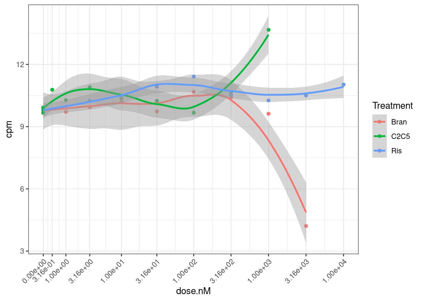

Ok, I can kind of understand how this the model fitting might be weird for this data.

Let’s try fitting model to logCPM now…

set.seed(0)
dat.fitted <-
  dat.tidy %>%
  sample_n_of(100, Treatment, gene) %>%
  group_by(Treatment, gene) %>% 
  # filter(hgnc_symbol=="STAT1") %>%
  # filter(hgnc_symbol %in% GenesOfInterest) %>%
  nest(-Treatment, -gene) %>%
  mutate(model = map(data, ~safe_drm(formula = log(cpm) ~ dose.nM,
                    data = .,
                    fct = LL.4(names=c("Steepness", "LowerLimit", "UpperLimit", "ED50"))))) %>%
  # filter out the wrapper functions that returned list with NA
  filter(!anyNA(model))

Error in optim(startVec, opfct, hessian = TRUE, method = optMethod, control = list(maxit = maxIt,  : 
  non-finite finite-difference value [4]

dat.fitted.summarised <- dat.fitted %>%
  mutate(results = map(model, tidy)) %>%
  unnest(results) %>%
  mutate(summary = map(model, glance)) %>%
  unnest(summary)

dat.fitted %>%
  mutate(resid = map(model, residuals)) %>%
  unnest(data, resid) %>%
  ggplot(aes(x=log(cpm), y=resid)) +
  coord_cartesian(xlim=c(0,6), ylim=c(-1,1)) +
  labs(title="Residuals as a function of CPM", caption="modelled CPM; not logCPM") +
  geom_point() +
  theme_bw()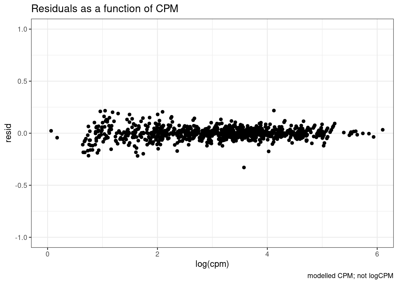

I think that is generally nicer… Let’s manually inspect dose response data points for genes of interest after log transforming the expression…

dat.tidy %>%
  filter(hgnc_symbol %in% GenesOfInterest) %>%
  ggplot(aes(x=dose.nM, y=log2(cpm), color=Treatment)) +
  geom_point() +
  geom_smooth(aes(group=Treatment), method = drm, method.args = list(fct = L.4(names=c("Steepness", "LowerLimit", "UpperLimit", "ED50"))), se = FALSE) +
  scale_x_continuous(trans="log1p", limits=c(0, 10000), breaks=c(10000, 3160, 1000, 316, 100, 31.6, 10, 3.16, 1, 0.316, 0)) +
  facet_wrap(~hgnc_symbol, scales="free_y") +
  theme_bw() +
  theme(axis.text.x = element_text(angle = 45, vjust = 1, hjust=1))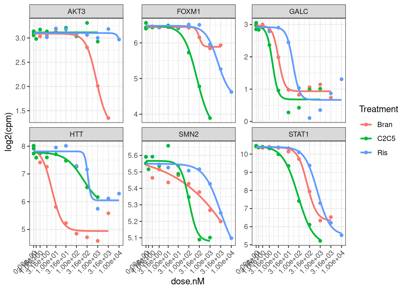

Hmm, based on these genes I’m still not sure if log transforming the CPM makes more sense, given that the field-standard model for dose-response curves is a sigmoidal shape log-logistic model. When viewed on this log-scale is notable that the effects keep going in terms of fold change, even at high doses… Contrast this to the same data plotted not on log-scale:

dat.tidy %>%
  filter(hgnc_symbol %in% GenesOfInterest) %>%
  ggplot(aes(x=dose.nM, y=cpm, color=Treatment)) +
  geom_point() +
  geom_smooth(aes(group=Treatment), method = drm, method.args = list(fct = L.4(names=c("Steepness", "LowerLimit", "UpperLimit", "ED50"))), se = FALSE) +
  scale_x_continuous(trans="log1p", limits=c(0, 10000), breaks=c(10000, 3160, 1000, 316, 100, 31.6, 10, 3.16, 1, 0.316, 0)) +
  facet_wrap(~hgnc_symbol, scales="free_y") +
  theme_bw() +
  theme(axis.text.x = element_text(angle = 45, vjust = 1, hjust=1))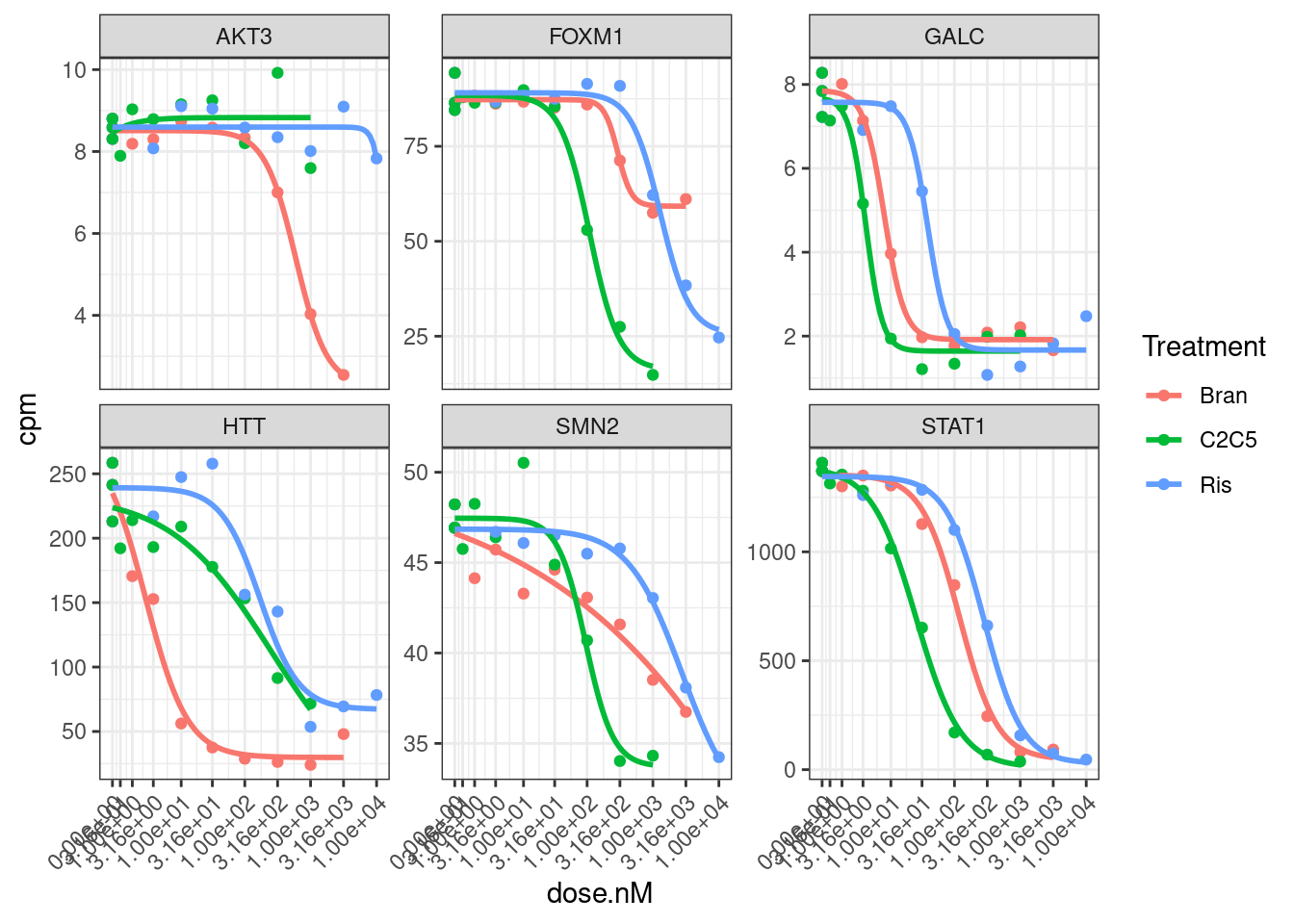

I think whether to log-transform the data almost depends on what we will do with the downstream analsis. Because the true effects on splicing still continue at low doses, so we might care most about as accurately modeling all these effects… In contrast, if we care about finding the genes therapeutic target genes, an effective knockdown might be better ascertained without log transform. Let’s fit a model to all gene:treatment combinations now and use log-transformed CPM as response variable.

Update: actually, this is a long computation for this notebook, let’s not evaluate this code block, and I’ll just use this notebook to prototype the model-fitting procedure before using a proper Rscript to fit models to all genes…

dat.fitted <-
  dat.tidy %>%
  group_by(Treatment, gene) %>% 
  nest(-Treatment, -gene) %>%
  mutate(model = map(data, ~safe_drm(formula = log2(cpm) ~ dose.nM,
                    data = .,
                    fct = LL.4(names=c("Steepness", "LowerLimit", "UpperLimit", "ED50"))))) %>%
  # filter out the wrapper functions that returned list with NA
  filter(!anyNA(model))

Let’s do some more careful comparisons between fit with log CPM versus CPM:

set.seed(0)
dat.fitted <-
  dat.tidy %>%
  sample_n_of(100, Treatment, gene) %>%
  group_by(Treatment, gene) %>% 
  # filter(hgnc_symbol=="STAT1") %>%
  # filter(hgnc_symbol %in% GenesOfInterest) %>%
  nest(-Treatment, -gene) %>%
  mutate(model.cpm.LL4 = map(data, ~safe_drm(formula = cpm ~ dose.nM,
                    data = .,
                    fct = LL.4(names=c("Steepness", "LowerLimit", "UpperLimit", "ED50"))))) %>%
  mutate(model.log2cpm.LL4 = map(data, ~safe_drm(formula = log2(cpm) ~ dose.nM,
                      data = .,
                      fct = LL.4(names=c("Steepness", "LowerLimit", "UpperLimit", "ED50"))))) %>%
  # filter out the wrapper functions that returned list with NA
  filter((!anyNA(model.cpm.LL4)) & (!anyNA(model.log2cpm.LL4))) %>%
  ungroup()

Error in optim(startVec, opfct, hessian = TRUE, method = optMethod, control = list(maxit = maxIt,  : 
  non-finite finite-difference value [4]
Error in optim(startVec, opfct, hessian = TRUE, method = optMethod, control = list(maxit = maxIt,  : 
  non-finite finite-difference value [4]

dat.fitted.summarised <- dat.fitted %>%
  gather(key="ModelName", value="model", model.cpm.LL4, model.log2cpm.LL4) %>%
  mutate(results = map(model, tidy)) %>%
  unnest(results) %>%
  mutate(summary = map(model, glance)) %>%
  unnest(summary)

dat.fitted.summarised %>%
  # select(gene, Treatment, ModelName, estimate, term)
  # spread(key="ModelName", value="estimate")
  mutate(estimate = case_when(
    (term %in% c("LowerLimit", "UpperLimit")) & (ModelName == "model.log2cpm.LL4") ~ 2**estimate,
    TRUE ~ estimate
  )) %>%
  pivot_wider(names_from = "ModelName", values_from="estimate", id_cols=c("gene", "Treatment", "term")) %>%
  ggplot(aes(x=model.cpm.LL4, y=model.log2cpm.LL4)) +
    geom_point() +
    scale_x_continuous(trans="log10") +
    scale_y_continuous(trans="log10") +
    facet_wrap(~term, scales="free") +
    theme_bw() +
    labs(title="Correlation of parameter point estimates with two models", caption="4 paramaeter log-logistic, modelling either logCPM or CPM\nLowerLimit and UpperLimit parameters converted to linear scale before plotting in log2CPM model")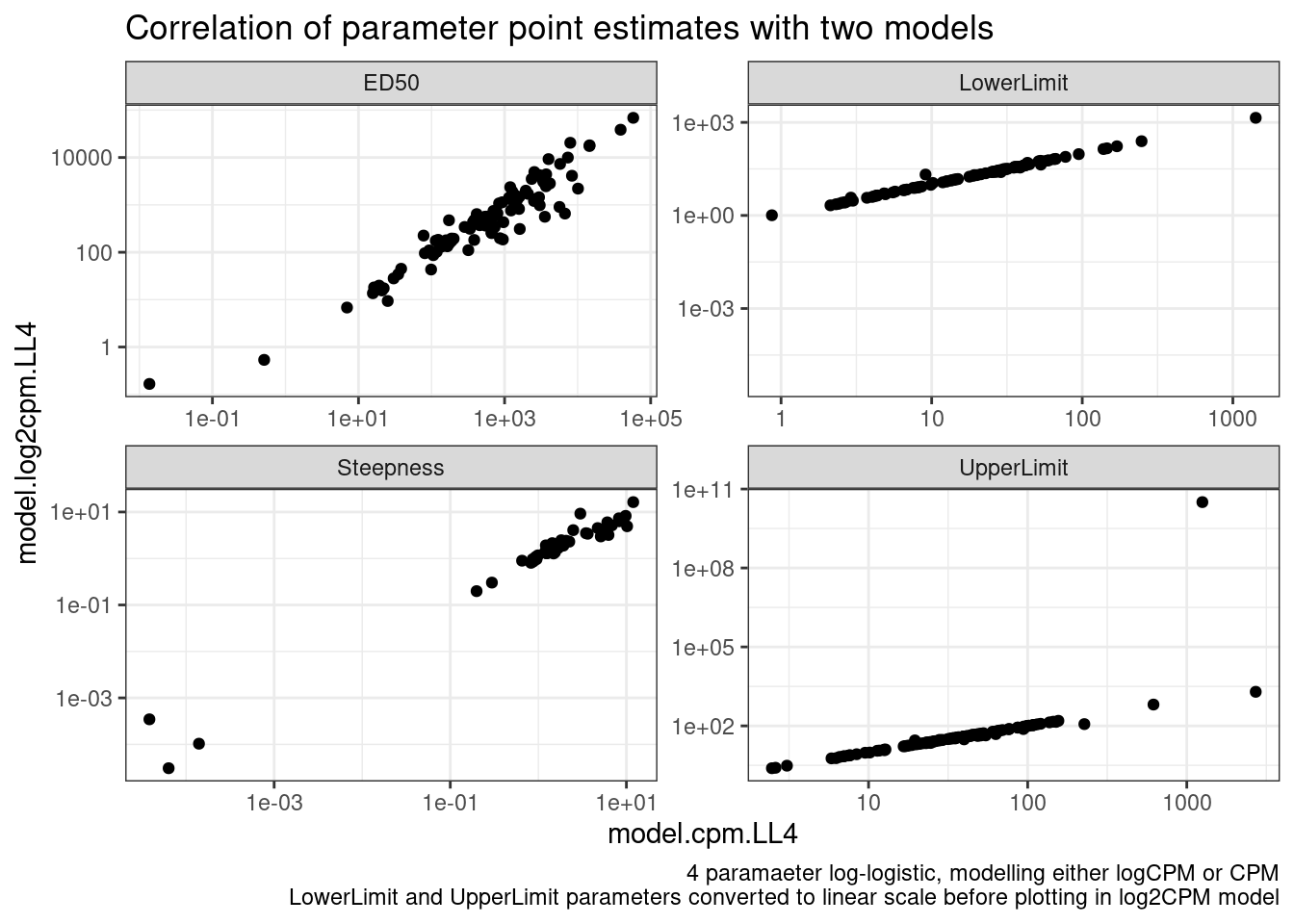

Ok, so the actual parameter estimates are more or less identical whether I model CPM or logCPM. In theory, heterskedastic erros should bias the paramater estiamtes, but only their standard errors.

Let’s compare AIC between the fit models versus simple linear regression.

mselect(fitted_curve, linreg=T)["Lin", "IC"]

[1] 28.95856

modelFit(fitted_curve)

Lack-of-fit test

          ModelDf      RSS Df F value p value
ANOVA           2 0.000487                   
DRC model       7 0.037384  5 30.2815  0.0323

plot(fitted_curve)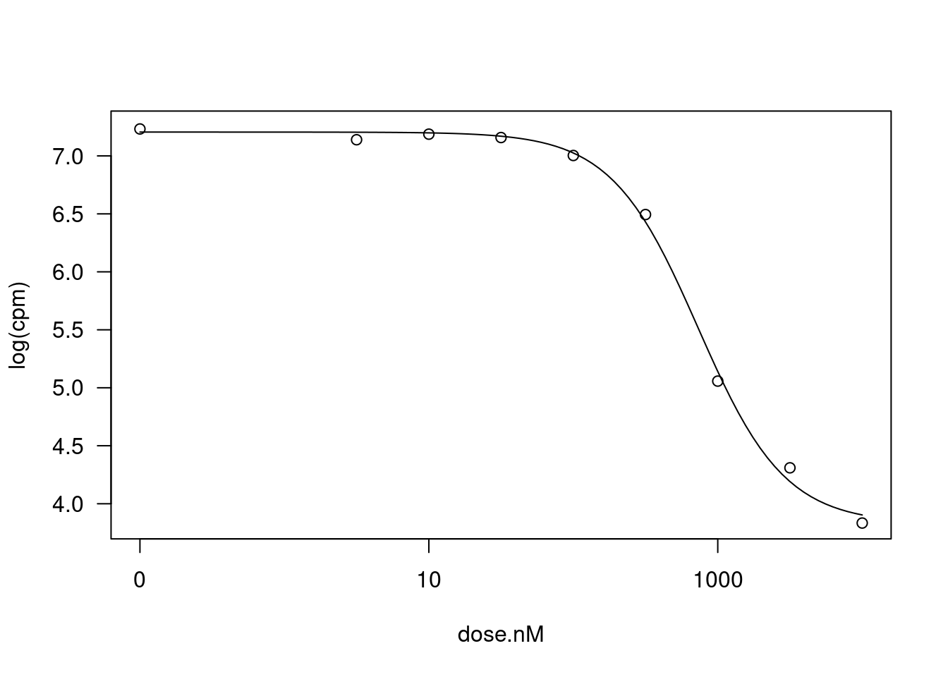

dat.fitted %>%
  gather(key="ModelName", value="model", model.cpm.LL4, model.log2cpm.LL4) %>%
  mutate(mselect.results = map(model, mselect, linreg=T)) %>%
  mutate(ModelFit = map(model, modelFit)) %>%
  rowwise() %>%
  mutate(DeltaAIC = mselect.results["LL.4", "IC"] - mselect.results["Lin", "IC"]) %>%
  rowwise() %>%
  mutate(Pval = ModelFit['DRC model', 'p value']) %>%
  ungroup() %>%
  ggplot(aes(x=DeltaAIC, fill=ModelName)) +
  geom_histogram() +
  theme_bw() +
  labs(x="Delta AIC with linear model", caption="More negative means better fit with LL.4 model")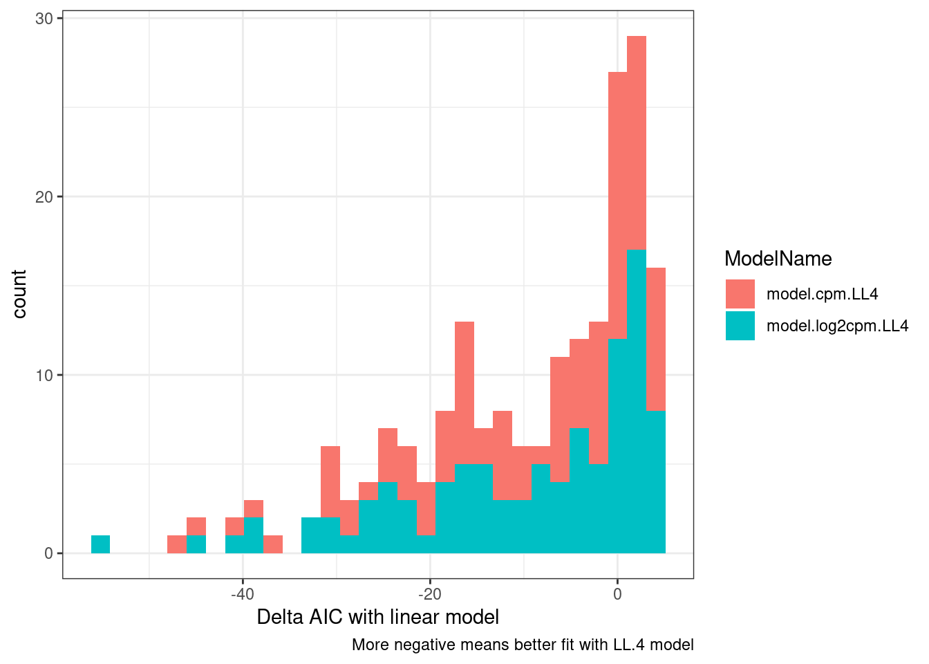

Let’s plot the original dose response points and the models and those model fit summary stats:

set.seed(1)
dat.fitted %>%
  gather(key="ModelName", value="model", model.cpm.LL4, model.log2cpm.LL4) %>%
  filter(ModelName == "model.log2cpm.LL4") %>%
  mutate(mselect.results = map(model, mselect, linreg=T)) %>%
  mutate(ModelFit = map(model, modelFit)) %>%
  rowwise() %>%
  mutate(DeltaAIC = mselect.results["LL.4", "IC"] - mselect.results["Lin", "IC"]) %>%
  rowwise() %>%
  mutate(Pval = ModelFit['DRC model', 'p value']) %>%
  ungroup() %>%
  sample_n(20) %>%
  unnest(data) %>%
  ggplot(aes(x=dose.nM, y=cpm, color=Treatment)) +
  geom_label(data = (
    . %>%
      distinct(Treatment, gene, .keep_all = T) %>%
      group_by(gene) %>%
      mutate(vjust = 1 * row_number()) %>%
      ungroup()),
    aes(label = paste0("DeltaAIC: ",signif(DeltaAIC,2), "\nP:", format.pval(Pval, digits = 2)), vjust=vjust),
    x=-Inf, y=Inf, size=3, hjust=-0.1
  ) +
  geom_point() +
  geom_smooth(aes(group=Treatment), method = drm, method.args = list(fct = L.4(names=c("Steepness", "LowerLimit", "UpperLimit", "ED50"))), se = FALSE) +
  scale_x_continuous(trans="log1p", limits=c(0, 10000), breaks=c(10000, 3160, 1000, 316, 100, 31.6, 10, 3.16, 1, 0.316, 0)) +
  facet_wrap(~hgnc_symbol, scales="free") +
  theme_bw() +
  theme(axis.text.x = element_text(angle = 45, vjust = 1, hjust=1))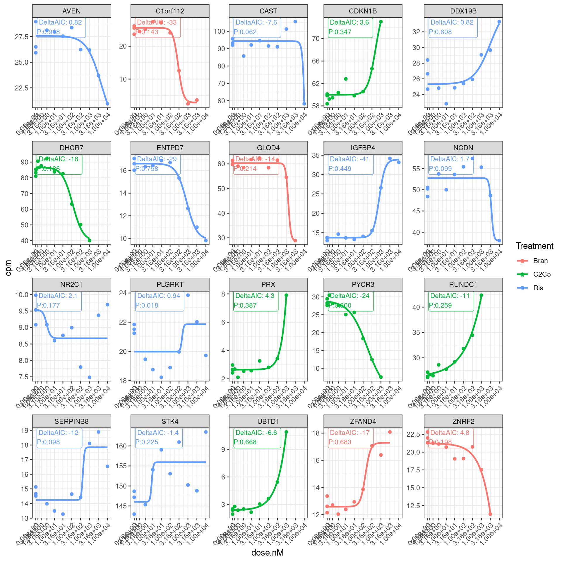

So a lot of things have a negative AIC (roughly meaning the four parameter log logistic model is better fit than simple linear model). The P value is also a test of if a simple anova model is better fit than the drc model, wherin small P-values indicate anova model is better. This practice of looking at actual curves and then inspecting the summary stats about how quality of the model is good.

Let me get some sense of the distribution of P values for this test

dat.fitted %>%
  gather(key="ModelName", value="model", model.cpm.LL4, model.log2cpm.LL4) %>%
  mutate(mselect.results = map(model, mselect, linreg=T)) %>%
  mutate(ModelFit = map(model, modelFit)) %>%
  rowwise() %>%
  mutate(DeltaAIC = mselect.results["LL.4", "IC"] - mselect.results["Lin", "IC"]) %>%
  rowwise() %>%
  mutate(Pval = ModelFit['DRC model', 'p value']) %>%
  ungroup() %>%
  ggplot(aes(x=Pval)) +
  geom_histogram(bins=20) +
  facet_wrap(~ModelName)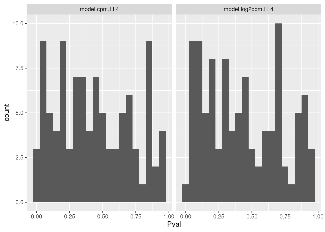

Ok that test might be reasonably calibrated. Maybe that is the simplest way I should evaluate goodness of fit.

Let’s also look at distribution of DeltaAIC

dat.fitted %>%
  gather(key="ModelName", value="model", model.cpm.LL4, model.log2cpm.LL4) %>%
  mutate(mselect.results = map(model, mselect, linreg=T)) %>%
  mutate(ModelFit = map(model, modelFit)) %>%
  rowwise() %>%
  mutate(DeltaAIC = mselect.results["LL.4", "IC"] - mselect.results["Lin", "IC"]) %>%
  rowwise() %>%
  mutate(Pval = ModelFit['DRC model', 'p value']) %>%
  ungroup() %>%
  ggplot(aes(x=DeltaAIC)) +
  geom_histogram(bins=20) +
  facet_wrap(~ModelName)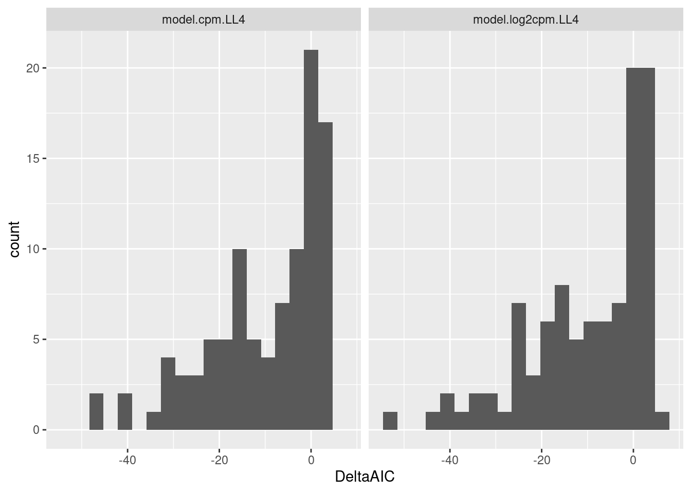

Let’s look at the raw data and fits for different ranges of DeltaAIC. From the previous plots a very negative deltaAIC might be a reasonable way to filter for reasonable fits.

Now I also want to inspect the standard errors of the parameter estimates. As before, I can either model logCPM as the response, or plain CPM and then use coeftest(fitted_curve, vcov = sandwich) to get more robust standard error estimates, instead of the biased standard errors (biased because of heterskedascity) output of drc.

coeftest(fitted_curve, vcov = sandwich)

t test of coefficients:

                         Estimate Std. Error t value  Pr(>|t|)    
Steepness:(Intercept)    1.446211   0.141243  10.239 1.830e-05 ***
LowerLimit:(Intercept)   3.828167   0.094068  40.696 1.410e-09 ***
UpperLimit:(Intercept)   7.205443   0.016000 450.344 < 2.2e-16 ***
ED50:(Intercept)       730.890420  58.873919  12.415 5.061e-06 ***
---
Signif. codes:  0 '***' 0.001 '**' 0.01 '*' 0.05 '.' 0.1 ' ' 1

dat.fitted %>%
  # head() %>%
  gather(key="ModelName", value="model", model.cpm.LL4, model.log2cpm.LL4) %>%
  mutate(results = map(model, tidy)) %>%
  mutate(results.robust = map(model, coeftest, vcov = sandwich)) %>%
  rowwise() %>%
  mutate(robust_estimate.Steepness = results.robust[1,1]) %>%
  mutate(robust_estimate.LowerLimit = results.robust[2,1]) %>%
  mutate(robust_estimate.UpperLimit = results.robust[3,1]) %>%
  mutate(robust_estimate.ED50 = results.robust[4,1]) %>%
  mutate(robust_se.Steepness = results.robust[1,2]) %>%
  mutate(robust_se.LowerLimit = results.robust[2,2]) %>%
  mutate(robust_se.UpperLimit = results.robust[3,2]) %>%
  mutate(robust_se.ED50 = results.robust[4,2]) %>%
  unnest(results) %>%
  pivot_longer(starts_with("robust_estimate"), names_to = "term2", names_prefix="robust_estimate.", values_to="robust.estimate") %>%
  filter(term==term2) %>%
  ggplot(aes(x=estimate, y=robust.estimate)) +
    geom_point() +
    scale_x_continuous(trans="log10") +
    scale_y_continuous(trans="log10") +
    facet_grid(rows=vars(ModelName), cols=vars(term)) +
    theme_bw() +
    labs(title="Correlation of parameter point estimates with two models and two estimate functions")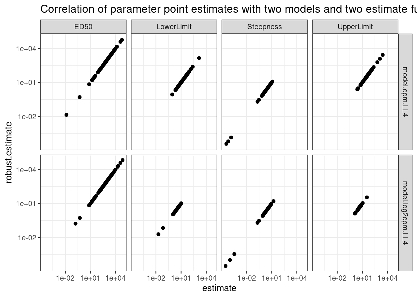

Ok, so clearly whether you use the standard drc output or the coeftest(fitted_curve, vcov = sandwich) (labelled as “robust estimate” above) you get the same number. Now check the same thing for standard error.

dat.fitted %>%
  # head() %>%
  gather(key="ModelName", value="model", model.cpm.LL4, model.log2cpm.LL4) %>%
  mutate(results = map(model, tidy)) %>%
  mutate(results.robust = map(model, coeftest, vcov = sandwich)) %>%
  rowwise() %>%
  mutate(robust_estimate.Steepness = results.robust[1,1]) %>%
  mutate(robust_estimate.LowerLimit = results.robust[2,1]) %>%
  mutate(robust_estimate.UpperLimit = results.robust[3,1]) %>%
  mutate(robust_estimate.ED50 = results.robust[4,1]) %>%
  mutate(robust_se.Steepness = results.robust[1,2]) %>%
  mutate(robust_se.LowerLimit = results.robust[2,2]) %>%
  mutate(robust_se.UpperLimit = results.robust[3,2]) %>%
  mutate(robust_se.ED50 = results.robust[4,2]) %>%
  unnest(results) %>%
  pivot_longer(starts_with("robust_se"), names_to = "term2", names_prefix="robust_se.", values_to="robust.se") %>%
  filter(term==term2) %>%
  ggplot(aes(x=std.error, y=robust.se)) +
    geom_abline(color="red") +
    geom_point() +
    scale_x_continuous(trans="log10") +
    scale_y_continuous(trans="log10") +
    facet_grid(rows=vars(ModelName), cols=vars(term)) +
    theme_bw() +
    labs(title="Correlation of parameter point estimates with two models and two estimate functions")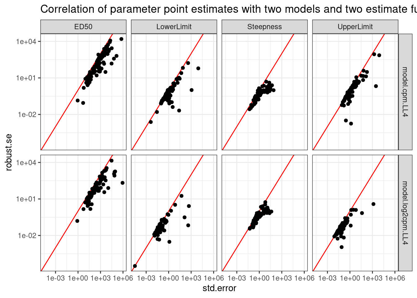

So the drc standard error can sometimes be upwardly biased, at least compared to the so called robust method. And this is true whether for both the logCPM and CPM models. I think I will just rely on the std error estimates directly from drc for simplicity, but I will use use the logCPM model.

Also one thing I can do is fit models for all the small molecule titration series at once, and tell drc that all three fits should have the same lower value (DMSO control). That seems the most proper way to use the DMSO samples.

dat.fitted.FixSameLowerLimit <- dat.tidy %>%
  # sample_n_of(100, Treatment, gene) %>%
  # group_by(Treatment, gene) %>% 
  # filter(hgnc_symbol=="STAT1") %>%
  filter(hgnc_symbol %in% GenesOfInterest) %>%
  nest(data=-gene) %>%
  mutate(model = map(data, ~safe_drm(formula = cpm ~ dose.nM,
                    curveid = Treatment,
                    data = .,
                    fct = LL.4(names=c("Steepness", "LowerLimit", "UpperLimit", "ED50")),
                    pmodels=data.frame(Treatment, 1, Treatment, Treatment)
                    ))) %>%
  # filter out the wrapper functions that returned list with NA
  filter(!anyNA(model))


dat.tidy.test <- dat.tidy %>%
  filter(hgnc_symbol=="RRM2B")
  # filter(hgnc_symbol=="STAT1")




fit <- drm(formula = cpm ~ dose.nM,
                    curveid = Treatment,
                    data = dat.tidy.test,
                    fct = LL.4(names=c("Steepness", "LowerLimit", "UpperLimit", "ED50")),
                    pmodels=data.frame(Treatment, 1, Treatment, Treatment))
plot(fit)

dat.tidy.test <- dat.tidy %>%
  filter(gene == "ENSG00000174574.16" & Treatment == "Bran")
fit <- drm(formula = cpm ~ dose.nM,
                    curveid = Treatment,
                    data = dat.tidy.test,
                    fct = LL.4(names=c("Steepness", "LowerLimit", "UpperLimit", "ED50")),
                    pmodels=data.frame(Treatment, Treatment, Treatment, Treatment))
plot(fit)
summary(fit)

Update:

• fitting models with the same lower limit (limit as dose approaches 0) is tricky because all the models are parameterised such that lower limit parameter is the defined as the the lower of the two limit parameters, so one would have to know ahead of time which parameter (the “LowerLimit” or the “UpperLimit” is the one that corresponds to limit as dose approaches 0).

For now let’s fit things as I have been doing, and start comparing parameter estimates between treatments.

set.seed(0)
dat.fitted <-
  dat.tidy %>%
  sample_n_of(100, gene) %>%
  group_by(Treatment, gene) %>% 
  # filter(hgnc_symbol=="STAT1") %>%
  # filter(hgnc_symbol %in% GenesOfInterest) %>%
  nest(-Treatment, -gene) %>%
  mutate(model.cpm.LL4 = map(data, ~safe_drm(formula = cpm ~ dose.nM,
                    data = .,
                    fct = LL.4(names=c("Steepness", "LowerLimit", "UpperLimit", "ED50"))))) %>%
  mutate(model.log2cpm.LL4 = map(data, ~safe_drm(formula = log2(cpm) ~ dose.nM,
                      data = .,
                      fct = LL.4(names=c("Steepness", "LowerLimit", "UpperLimit", "ED50"))))) %>%
  # filter out the wrapper functions that returned list with NA
  filter((!anyNA(model.cpm.LL4)) & (!anyNA(model.log2cpm.LL4))) %>%
  ungroup()

Error in optim(startVec, opfct, hessian = TRUE, method = optMethod, control = list(maxit = maxIt,  : 
  non-finite finite-difference value [4]
Error in optim(startVec, opfct, hessian = TRUE, method = optMethod, control = list(maxit = maxIt,  : 
  non-finite finite-difference value [1]
Error in optim(startVec, opfct, hessian = TRUE, method = optMethod, control = list(maxit = maxIt,  : 
  non-finite finite-difference value [4]
Error in optim(startVec, opfct, hessian = TRUE, method = optMethod, control = list(maxit = maxIt,  : 
  non-finite finite-difference value [1]

dat.to.plot <- dat.fitted %>%
  gather(key="ModelName", value="model", model.cpm.LL4, model.log2cpm.LL4) %>%
  filter(ModelName == "model.log2cpm.LL4") %>%
  mutate(results = map(model, tidy)) %>%
  mutate(mselect.results = map(model, mselect, linreg=T)) %>%
  mutate(ModelFit = map(model, modelFit)) %>%
  rowwise() %>%
  mutate(DeltaAIC = mselect.results["LL.4", "IC"] - mselect.results["Lin", "IC"]) %>%
  rowwise() %>%
  mutate(Pval = ModelFit['DRC model', 'p value']) %>%
  unnest(results) %>%
  filter(Treatment %in% c("Ris", "Bran")) %>%
  dplyr::select(Treatment, gene, estimate, std.error, Pval, DeltaAIC, term)
  # spread(Treatment, estimate)
  
  

dat.to.plot %>%
  pivot_wider(names_from=c("Treatment"), values_from=c("estimate", "std.error", "Pval", "DeltaAIC"), id_cols=c("gene", "term")) %>%
  drop_na() %>%
  ggplot(aes(x=DeltaAIC_Bran, DeltaAIC_Ris)) +
  geom_point() +
    theme_bw()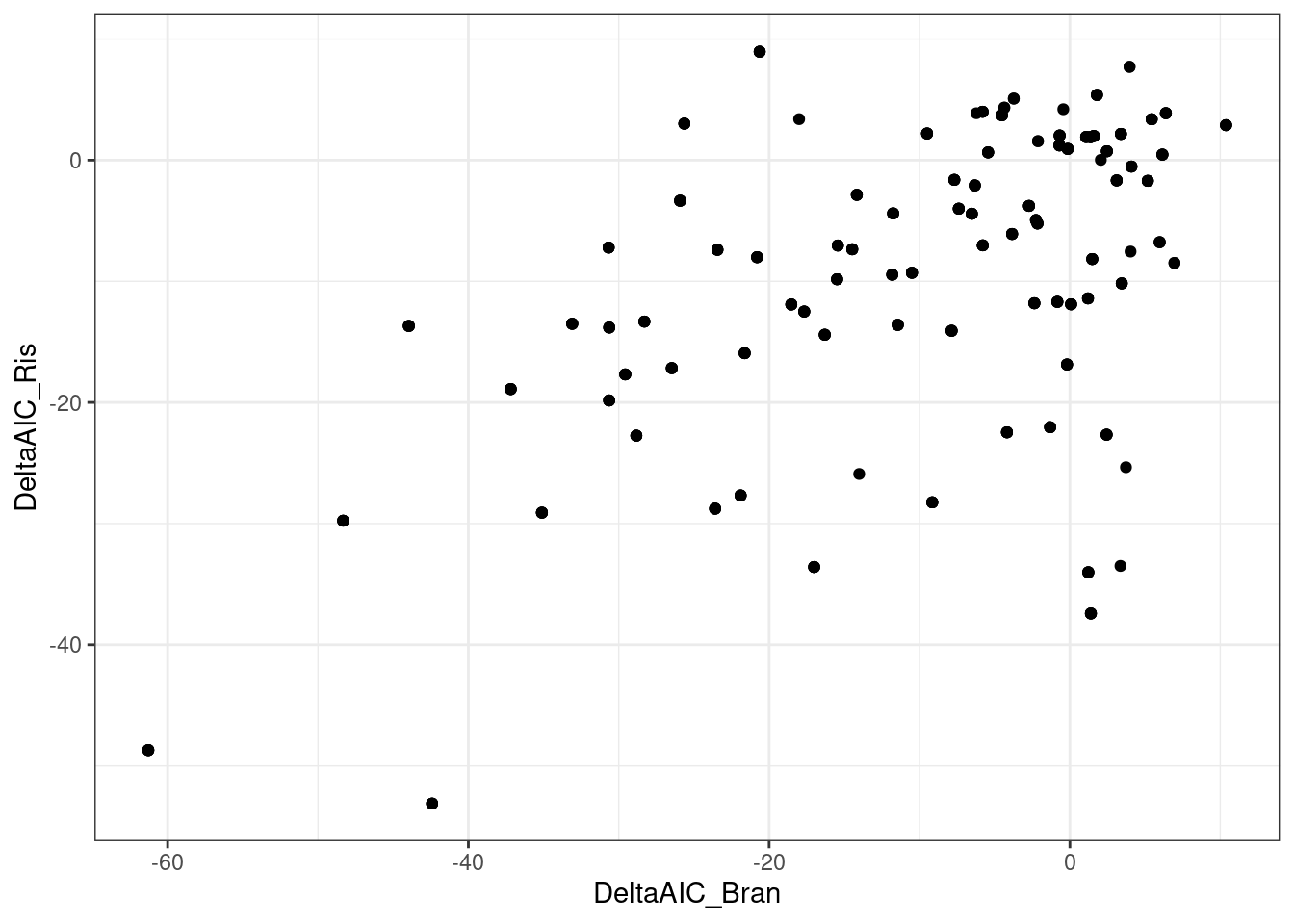

dat.to.plot %>%
  pivot_wider(names_from=c("Treatment"), values_from=c("estimate", "std.error", "Pval", "DeltaAIC"), id_cols=c("gene", "term")) %>%
  drop_na() %>%
  ggplot(aes(x=-log10(Pval_Bran), -log10(Pval_Ris))) +
  geom_point() +
    theme_bw()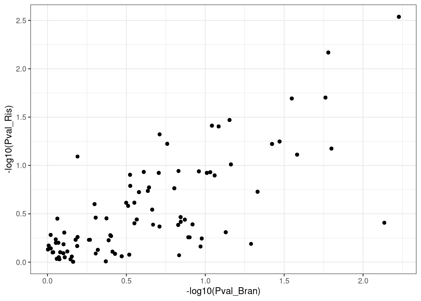

dat.to.plot %>%
  pivot_wider(names_from=c("Treatment"), values_from=c("estimate", "std.error", "Pval", "DeltaAIC"), id_cols=c("gene", "term")) %>%
  drop_na() %>%
  ggplot(aes(x=-log10(Pval_Bran), y=DeltaAIC_Bran)) +
  geom_point() +
    theme_bw()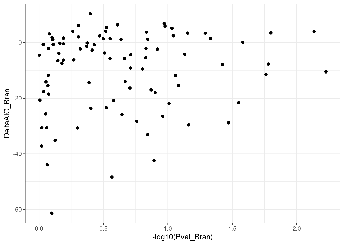

dat.to.plot %>%
  pivot_wider(names_from=c("Treatment"), values_from=c("estimate", "std.error", "Pval", "DeltaAIC"), id_cols=c("gene", "term")) %>%
  drop_na() %>%
  rowwise() %>%
  mutate(meanDeltaAIC = mean(DeltaAIC_Ris, DeltaAIC_Bran)) %>%
  ungroup() %>%
  ggplot(aes(x=estimate_Bran, y=estimate_Ris, color=meanDeltaAIC)) +
  geom_abline() +
  geom_errorbar(aes(xmin = estimate_Bran-std.error_Bran, xmax=estimate_Bran+std.error_Bran)) +
  geom_errorbar(aes(ymin = estimate_Ris-std.error_Ris, ymax=estimate_Ris+std.error_Ris)) +
  geom_point() +
  scale_x_continuous(trans="log10") +
  scale_y_continuous(trans="log10") +
  facet_wrap(~term, scales="free") +
  theme_bw()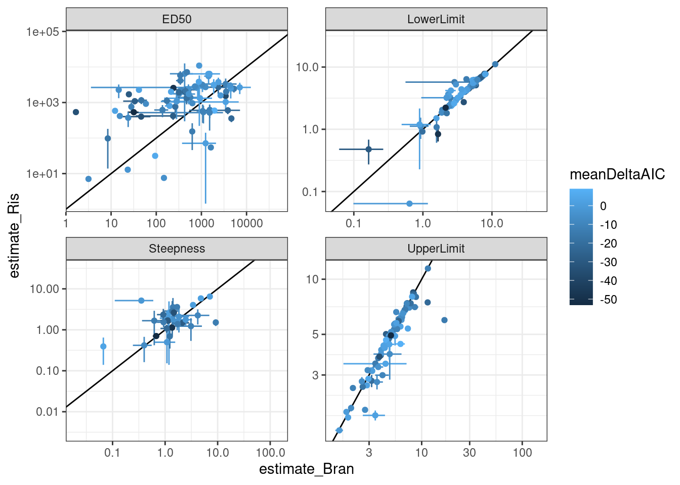

Let’s check out some individual models for individual points on these plots… starting with this red point

PointsOfInterest <- dat.to.plot %>%
  filter(term=="ED50" & Treatment == "Bran" & estimate <5) %>%
  pull(gene)

dat.to.plot %>%
  pivot_wider(names_from=c("Treatment"), values_from=c("estimate", "std.error", "Pval", "DeltaAIC"), id_cols=c("gene", "term")) %>%
  drop_na() %>%
  rowwise() %>%
  mutate(meanDeltaAIC = mean(DeltaAIC_Ris, DeltaAIC_Bran)) %>%
  ungroup() %>%
  mutate(IsPointOfInterest = gene %in% PointsOfInterest) %>%
  ggplot(aes(x=estimate_Bran, y=estimate_Ris, color=IsPointOfInterest)) +
  geom_abline() +
  geom_errorbar(aes(xmin = estimate_Bran-std.error_Bran, xmax=estimate_Bran+std.error_Bran)) +
  geom_errorbar(aes(ymin = estimate_Ris-std.error_Ris, ymax=estimate_Ris+std.error_Ris)) +
  geom_point() +
  # geom_text(aes(label=gene), size=2) +
  scale_x_continuous(trans="log10") +
  scale_y_continuous(trans="log10") +
  facet_wrap(~term, scales="free") +
  theme_bw()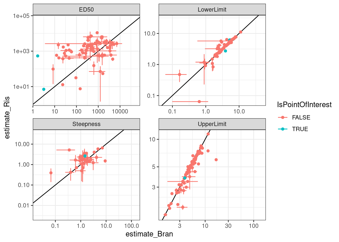

dat.tidy.test <- dat.tidy %>%
  filter(gene == "ENSG00000160117.16")
fit <- drm(formula = log2(cpm) ~ dose.nM,
                    curveid = Treatment,
                    data = dat.tidy.test,
                    fct = LL.4(names=c("Steepness", "LowerLimit", "UpperLimit", "ED50")),
                    pmodels=data.frame(Treatment, Treatment, Treatment, Treatment))
plot(fit)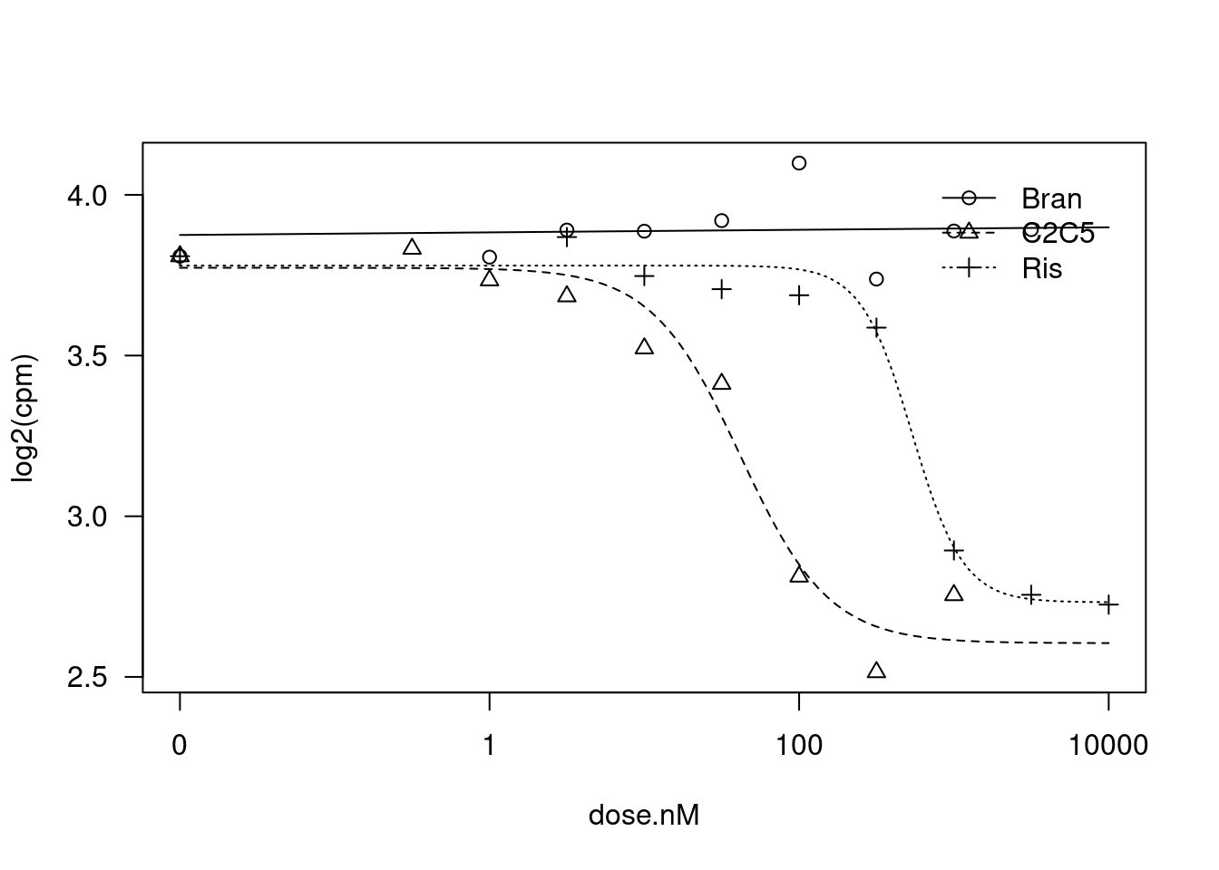

summary(fit)

Model fitted: Log-logistic (ED50 as parameter) (4 parms)

Parameter estimates:

                  Estimate Std. Error  t-value   p-value    
Steepness:Bran    0.050718   0.471413   0.1076 0.9153451    
Steepness:C2C5    1.517828   0.573221   2.6479 0.0150467 *  
Steepness:Ris     2.648206   0.948493   2.7920 0.0109234 *  
LowerLimit:Bran   3.948101   0.232945  16.9486 9.989e-14 ***
LowerLimit:C2C5   2.605019   0.080378  32.4096 < 2.2e-16 ***
LowerLimit:Ris    2.732253   0.072514  37.6790 < 2.2e-16 ***
UpperLimit:Bran   3.808415   0.055072  69.1534 < 2.2e-16 ***
UpperLimit:C2C5   3.773050   0.045628  82.6912 < 2.2e-16 ***
UpperLimit:Ris    3.779937   0.037193 101.6307 < 2.2e-16 ***
ED50:Bran         0.059997   2.801106   0.0214 0.9831136    
ED50:C2C5        41.666034   9.529184   4.3725 0.0002667 ***
ED50:Ris        537.947942 103.762622   5.1844 3.883e-05 ***
---
Signif. codes:  0 '***' 0.001 '**' 0.01 '*' 0.05 '.' 0.1 ' ' 1

Residual standard error:

 0.09576291 (21 degrees of freedom)

dat.tidy.test <- dat.tidy %>%
  filter(gene == "ENSG00000075239.14")
fit <- drm(formula = log2(cpm) ~ dose.nM,
                    curveid = Treatment,
                    data = dat.tidy.test,
                    fct = LL.4(names=c("Steepness", "LowerLimit", "UpperLimit", "ED50")),
                    pmodels=data.frame(Treatment, Treatment, Treatment, Treatment))
plot(fit)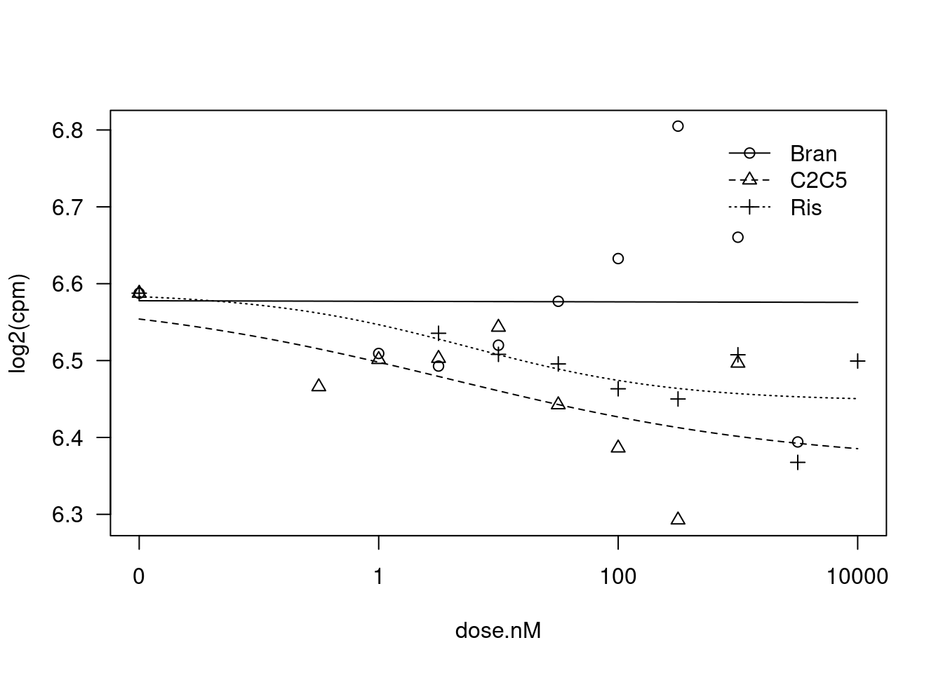

summary(fit)

Model fitted: Log-logistic (ED50 as parameter) (4 parms)

Parameter estimates:

                 Estimate Std. Error  t-value p-value    
Steepness:Bran   0.081277         NA       NA      NA    
Steepness:C2C5   0.297441   0.500894   0.5938  0.5590    
Steepness:Ris    0.500408   1.221937   0.4095  0.6863    
LowerLimit:Bran  6.573052   0.014816 443.6547  <2e-16 ***
LowerLimit:C2C5  6.366048   0.170200  37.4034  <2e-16 ***
LowerLimit:Ris   6.447259   0.074544  86.4891  <2e-16 ***
UpperLimit:Bran  6.580825   0.026813 245.4363  <2e-16 ***
UpperLimit:C2C5  6.585943   0.053893 122.2048  <2e-16 ***
UpperLimit:Ris   6.588939   0.051593 127.7093  <2e-16 ***
ED50:Bran        3.228366         NA       NA      NA    
ED50:C2C5        3.887193  23.120871   0.1681  0.8681    
ED50:Ris         5.534319  21.279802   0.2601  0.7973    
---
Signif. codes:  0 '***' 0.001 '**' 0.01 '*' 0.05 '.' 0.1 ' ' 1

Residual standard error:

 0.09086537 (21 degrees of freedom)

dat.tidy.test <- dat.tidy %>%
  filter(gene == "ENSG00000136436.14")
fit <- drm(formula = log2(cpm) ~ dose.nM,
                    curveid = Treatment,
                    data = dat.tidy.test,
                    fct = LL.4(names=c("Steepness", "LowerLimit", "UpperLimit", "ED50")),
                    pmodels=data.frame(Treatment, Treatment, Treatment, Treatment))
plot(fit)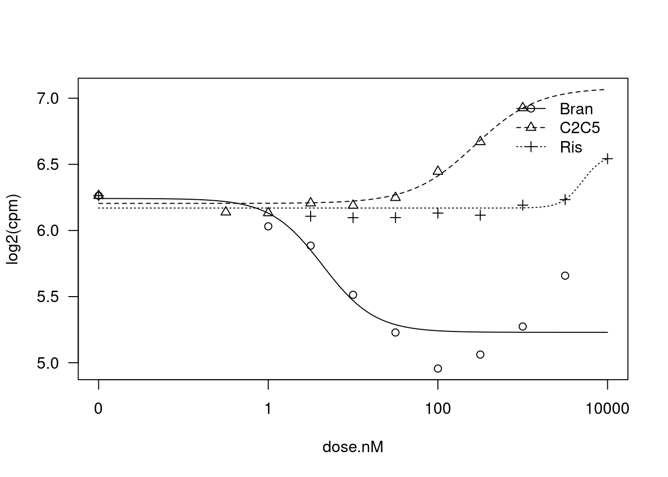

summary(fit)

Model fitted: Log-logistic (ED50 as parameter) (4 parms)

Parameter estimates:

                   Estimate  Std. Error  t-value   p-value    
Steepness:Bran     1.416690    0.542319   2.6123   0.01627 *  
Steepness:C2C5    -1.176207    1.031273  -1.1405   0.26690    
Steepness:Ris     -3.540543          NA       NA        NA    
LowerLimit:Bran    5.230006    0.068466  76.3883 < 2.2e-16 ***
LowerLimit:C2C5    6.204725    0.056185 110.4344 < 2.2e-16 ***
LowerLimit:Ris     6.169790    0.047715 129.3052 < 2.2e-16 ***
UpperLimit:Bran    6.241918    0.083875  74.4191 < 2.2e-16 ***
UpperLimit:C2C5    7.078879    0.568146  12.4596  3.63e-11 ***
UpperLimit:Ris     6.576517          NA       NA        NA    
ED50:Bran          4.379765    1.789508   2.4475   0.02327 *  
ED50:C2C5        269.370620  408.653096   0.6592   0.51695    
ED50:Ris        5068.662728          NA       NA        NA    
---
Signif. codes:  0 '***' 0.001 '**' 0.01 '*' 0.05 '.' 0.1 ' ' 1

Residual standard error:

 0.1437782 (21 degrees of freedom)

Ok, lot’s of interseting things going on.

Session information

sessionInfo()

R version 3.6.1 (2019-07-05)
Platform: x86_64-pc-linux-gnu (64-bit)
Running under: Scientific Linux 7.4 (Nitrogen)

Matrix products: default
BLAS/LAPACK: /software/openblas-0.2.19-el7-x86_64/lib/libopenblas_haswellp-r0.2.19.so

locale:
 [1] LC_CTYPE=en_US.UTF-8       LC_NUMERIC=C              
 [3] LC_TIME=en_US.UTF-8        LC_COLLATE=en_US.UTF-8    
 [5] LC_MONETARY=en_US.UTF-8    LC_MESSAGES=en_US.UTF-8   
 [7] LC_PAPER=en_US.UTF-8       LC_NAME=C                 
 [9] LC_ADDRESS=C               LC_TELEPHONE=C            
[11] LC_MEASUREMENT=en_US.UTF-8 LC_IDENTIFICATION=C       

attached base packages:
[1] stats     graphics  grDevices utils     datasets  methods   base     

other attached packages:
 [1] lmtest_0.9-37      zoo_1.8-10         sandwich_3.0-2     drc_3.0-1         
 [5] MASS_7.3-51.4      qvalue_2.16.0      broom_1.0.0        viridis_0.5.1     
 [9] viridisLite_0.3.0  gplots_3.0.1.1     RColorBrewer_1.1-2 edgeR_3.26.5      
[13] limma_3.40.6       forcats_0.4.0      stringr_1.4.0      dplyr_1.0.9       
[17] purrr_0.3.4        readr_1.3.1        tidyr_1.2.0        tibble_3.1.7      
[21] ggplot2_3.3.6      tidyverse_1.3.0   

loaded via a namespace (and not attached):
 [1] nlme_3.1-140       bitops_1.0-6       fs_1.3.1           lubridate_1.7.4   
 [5] httr_1.4.1         rprojroot_2.0.2    tools_3.6.1        backports_1.4.1   
 [9] utf8_1.1.4         R6_2.4.0           KernSmooth_2.23-15 mgcv_1.8-40       
[13] DBI_1.1.0          colorspace_1.4-1   withr_2.4.1        tidyselect_1.1.2  
[17] gridExtra_2.3      curl_3.3           compiler_3.6.1     git2r_0.26.1      
[21] cli_3.3.0          rvest_0.3.5        xml2_1.3.2         labeling_0.3      
[25] caTools_1.17.1.2   scales_1.1.0       mvtnorm_1.1-3      digest_0.6.20     
[29] foreign_0.8-71     rmarkdown_1.13     rio_0.5.16         pkgconfig_2.0.2   
[33] htmltools_0.3.6    plotrix_3.8-2      highr_0.9          dbplyr_1.4.2      
[37] rlang_1.0.3        readxl_1.3.1       rstudioapi_0.10    farver_2.1.0      
[41] generics_0.1.3     jsonlite_1.6       gtools_3.9.2.2     zip_2.0.3         
[45] car_3.0-5          magrittr_1.5       Matrix_1.2-18      Rcpp_1.0.5        
[49] munsell_0.5.0      fansi_0.4.0        abind_1.4-5        lifecycle_1.0.1   
[53] multcomp_1.4-19    stringi_1.4.3      yaml_2.2.0         carData_3.0-5     
[57] plyr_1.8.4         grid_3.6.1         gdata_2.18.0       promises_1.0.1    
[61] crayon_1.3.4       lattice_0.20-38    haven_2.3.1        splines_3.6.1     
[65] hms_0.5.3          locfit_1.5-9.1     knitr_1.39         pillar_1.7.0      
[69] codetools_0.2-18   reshape2_1.4.3     reprex_0.3.0       glue_1.6.2        
[73] evaluate_0.15      data.table_1.14.2  modelr_0.1.8       vctrs_0.4.1       
[77] httpuv_1.5.1       cellranger_1.1.0   gtable_0.3.0       assertthat_0.2.1  
[81] xfun_0.31          openxlsx_4.1.0.1   later_0.8.0        survival_2.44-1.1 
[85] workflowr_1.6.2    TH.data_1.1-1      ellipsis_0.3.2