CompareFibroblastToLCL_DE

Intro

I previously performed DE analysis in small molecule treated fibroblasts, and calculated correlation coefficients across dose-response data in LCLs… How do the measured effects between these two cell types compare. At the gene level? At the splicing level?

At the splicing level I strongly hypothesize signs of effects to be concordant. After all, the known mechanism for these molecules are by modifying U1:5’ss interaction, and since U1 is a ubiquitous factor in splicing (as opposed to say cell-type specific splice factors), I expect that an 5’ss that is enhanced in one cell type will similarly be enhanced in another. though because of cell-type-sepcific expressed genes, some introns just won’t be captured/measured well in all cell types. And to some degree, there may be some cell-type specific factors that determine which cryptic splice sites have activation potential, again meaning that not all introns will be captured efficiently in different cell types, but the sign of effects (that we can measure) should be very concordant.

As for gene expression, I am a bit less sure how concordant things will be… When small molecule induces a poison exon in a gene that downregulates expression in one cell type, are there other down-regulating (poison) or up-regulating induced exons that trump the first effect because of their stronger inclusion level?

Let’s read in the data… starting with gene expression data

library(tidyverse)

DE.fibroblast.dat <- read_tsv("../code/DE_testing/Results.txt.gz") %>%
  separate(Geneid, into=c("EnsemblID", "GeneSymbol"), sep = "_")

Expression.LCL.dat <- read_tsv("../code/DoseResponseData/LCL/TidyExpressionDoseData.txt.gz")

Note that the small molecules used in the fibroblast data aren’t exactly the same as in the LCL dose response series. From looking at a number of branaplam-specific and rsidiplam-specific splice events (determined as such in LCLs) in the fibroblast data, I can tell that SM2 is most like branaplam. For now, let’s keep our comparisons between cell types to comparing these two similar molecules.

First I’ll compare significant DE genes (in fibroblast) to the spearman correlation coef in LCLs across the dose response series, limiting to genes that are reasonable expressed.

GenesExpressedInLCLs <- Expression.LCL.dat %>%
  group_by(Geneid) %>%
  filter(max(CPM) > 1) %>%
  pull(Geneid) %>% unique()

DE.fibroblast.dat %>%
  filter(treatment == "SM2") %>%
  inner_join(
    Expression.LCL.dat %>%
      filter(treatment == "Branaplam") %>%
      distinct(Geneid, treatment, .keep_all=T),
    by=c("EnsemblID"="Geneid")
  ) %>%
  filter(FDR < 0.01) %>%
  filter(EnsemblID %in% GenesExpressedInLCLs) %>%
  ggplot(aes(x=logFC, y=spearman)) +
  geom_point(alpha=0.1) +
  theme_bw()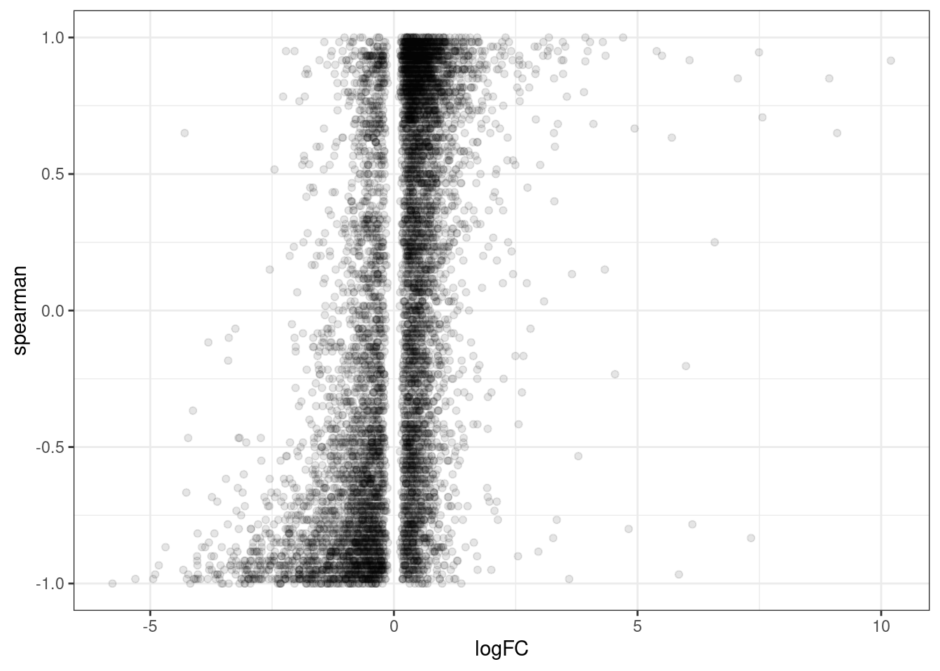

Ok, there is clearly some positive correlation. That’s reassuring somewhat. It’s pretty busy with low effect things that are hard to interpret in this messy plot. Let’s replot, just focusing on larger effect sizes, say greater than 2 fold change:

DE.fibroblast.dat %>%
  filter(treatment == "SM2") %>%
  inner_join(
    Expression.LCL.dat %>%
      filter(treatment == "Branaplam") %>%
      distinct(Geneid, treatment, .keep_all=T),
    by=c("EnsemblID"="Geneid")
  ) %>%
  filter(FDR < 0.01) %>%
  filter(abs(logFC)>1) %>%
  filter(EnsemblID %in% GenesExpressedInLCLs) %>%
  ggplot(aes(x=logFC, y=spearman)) +
  geom_point(alpha=0.1) +
  theme_bw()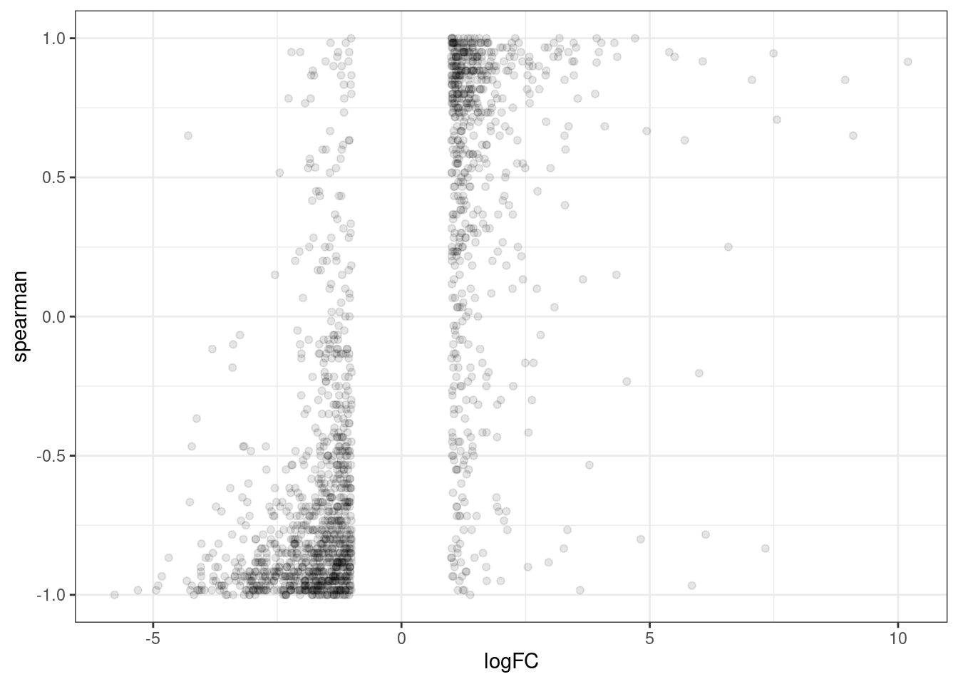

Ok, maybe to get a better intuition, let’s calculate the number of concordant sign changes versus nonconcorant.

DE.fibroblast.dat %>%
  filter(treatment == "SM2") %>%
  inner_join(
    Expression.LCL.dat %>%
      filter(treatment == "Branaplam") %>%
      distinct(Geneid, treatment, .keep_all=T),
    by=c("EnsemblID"="Geneid")
  ) %>%
  filter(FDR < 0.01) %>%
  filter(abs(logFC)>1) %>%
  mutate(Concordant = sign(logFC)==sign(spearman)) %>%
  count(Concordant)

# A tibble: 3 × 2
  Concordant     n
  <lgl>      <int>
1 FALSE        585
2 TRUE        2138
3 NA           118

Ok, about 80% concordant signs. that’s pretty good I’d say.

Let’s also limit to abs(spearman)>0.9, which I have been using as a quick way to filter for genes/introns even worth modelling.

DE.fibroblast.dat %>%
  filter(treatment == "SM2") %>%
  inner_join(
    Expression.LCL.dat %>%
      filter(treatment == "Branaplam") %>%
      distinct(Geneid, treatment, .keep_all=T),
    by=c("EnsemblID"="Geneid")
  ) %>%
  filter(FDR < 0.01) %>%
  filter(abs(logFC)>1) %>%
  filter(abs(spearman)>0.9) %>%
  mutate(Concordant = sign(logFC)==sign(spearman)) %>%
  count(Concordant)

# A tibble: 2 × 2
  Concordant     n
  <lgl>      <int>
1 FALSE         30
2 TRUE         509

Ok, close to about 90% concordance.

Let’s do some of the same type of analysis for splicing of introns.

First, to read in the fibroblast leafcutter differential splicing results…

cluster_sig_files <- list.files("../code/SplicingAnalysis/leafcutter/differential_splicing", "*_cluster_significance.txt", full.names = T)
effect_sizes_files <- list.files("../code/SplicingAnalysis/leafcutter/differential_splicing", "*_effect_sizes.txt", full.names = T)
treatments <- str_replace(cluster_sig_files, ".+/(.+?)_cluster_significance.txt", "\\1")

cluster.sig <- map(cluster_sig_files, read_tsv) %>%
  set_names(cluster_sig_files) %>%
  bind_rows(.id="f") %>%
  mutate(treatment = str_replace(f, ".+/(.+?)_cluster_significance.txt", "\\1")) %>%
  dplyr::select(-f)

effect_sizes <- map(effect_sizes_files, read_tsv) %>%
  set_names(effect_sizes_files) %>%
  bind_rows(.id="f") %>%
  mutate(treatment = str_replace(f, ".+/(.+?)_effect_sizes.txt", "\\1")) %>%
  dplyr::select(-f) %>%
  unite("psi_treatment", treatments, sep=" ", na.rm=T) %>%
  mutate(psi_treatment = as.numeric(psi_treatment),
         cluster = str_replace(intron, "(.+?:).+:(.+?)", "\\1\\2"))

#Switch sign, so that positive means increase in treatment
effect_sizes <- effect_sizes %>%
  mutate(deltapsi = deltapsi*-1,
         logef = logef *-1)

#Combine effect sizes and significance for all samples into single df
leafcutter.ds <- effect_sizes %>%
  left_join(cluster.sig, by=c("treatment", "cluster"))

Now read in the LCL dose by intronPSI spearman correlation coefficients

Splicing.LCL.dat <- read_tsv("../code/DoseResponseData/LCL/TidySplicingDoseData.txt.gz")

dat.to.plot <- Splicing.LCL.dat %>%
  filter(treatment == "Branaplam") %>%
  group_by(junc) %>%
  filter(max(PSI) > 10) %>%
  ungroup() %>%
  distinct(junc, treatment, .keep_all=T) %>%
  inner_join(
    leafcutter.ds %>%
      filter(treatment == "SM2") %>%
      separate(intron, into=c("#Chrom", "start", "end", "FibroblastCluster"), convert=T, sep=":"),
    by=c("#Chrom", "start", "end")
  ) %>%
  filter(p.adjust < 0.01)
dat.to.plot %>%
  mutate(Concordant = sign(deltapsi)==sign(spearman)) %>%
  count(Concordant)

# A tibble: 3 × 2
  Concordant     n
  <lgl>      <int>
1 FALSE       2863
2 TRUE        9585
3 NA            35

ggplot(dat.to.plot, aes(x=deltapsi, y=spearman)) +
  geom_point(alpha=0.1) +
  theme_bw() +
  labs(caption="Filtering for fibroblast FDR<1%",
       x="deltapsi in fibroblast", y='spearman coef in LCL dose response series')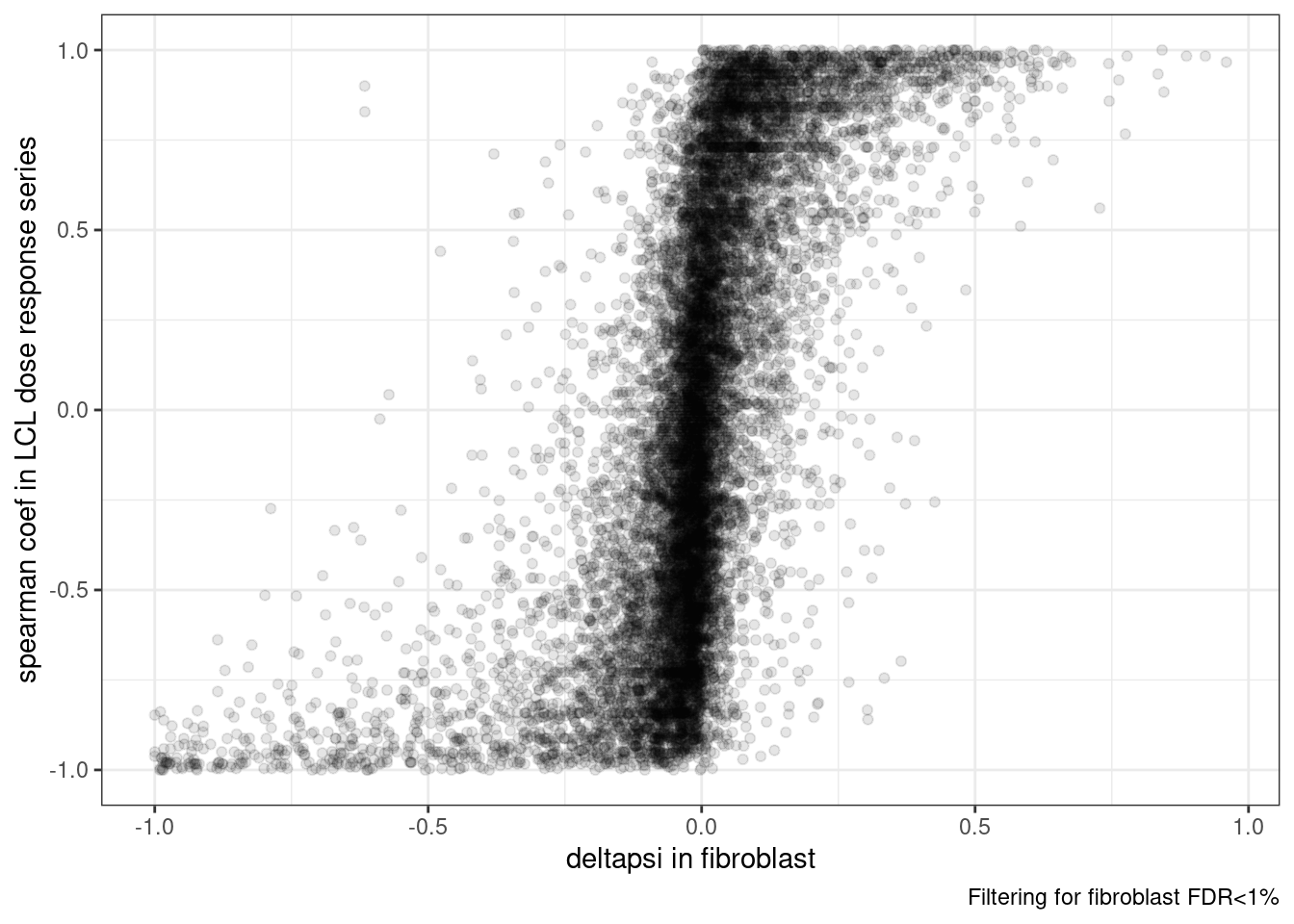

dat.to.plot <- Splicing.LCL.dat %>%
  filter(treatment == "Branaplam") %>%
  group_by(junc) %>%
  filter(max(PSI) > 10) %>%
  ungroup() %>%
  distinct(junc, treatment, .keep_all=T) %>%
  inner_join(
    leafcutter.ds %>%
      filter(treatment == "SM2") %>%
      separate(intron, into=c("#Chrom", "start", "end", "FibroblastCluster"), convert=T, sep=":"),
    by=c("#Chrom", "start", "end")
  ) %>%
  filter(p.adjust < 0.01) %>%
  filter(abs(deltapsi)>0.1)
dat.to.plot %>%
  mutate(Concordant = sign(deltapsi)==sign(spearman)) %>%
  count(Concordant)

# A tibble: 3 × 2
  Concordant     n
  <lgl>      <int>
1 FALSE        331
2 TRUE        3657
3 NA             5

ggplot(dat.to.plot, aes(x=deltapsi, y=spearman)) +
  geom_point(alpha=0.1) +
  theme_bw() +
  labs(caption="Filtering for fibroblast deltaPSI>10% and FDR<1%",
       x="deltapsi in fibroblast", y='spearman coef in LCL dose response series')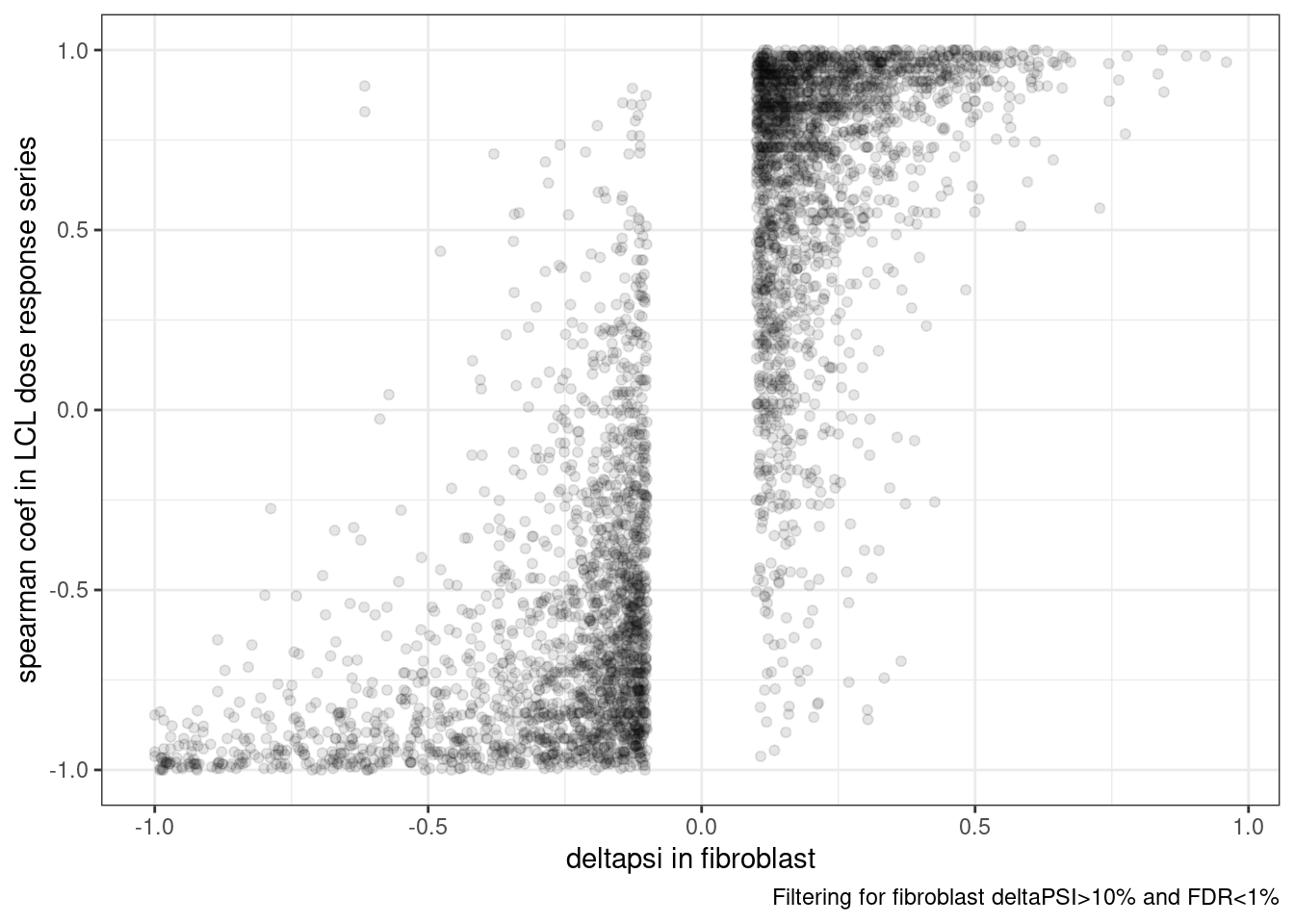

Conclusion

I think it is fair to for the most part that a detected change in one cell type will not change sign in a different cell type. So to me, the point of assaying different cell types is more to gain power in cell-type-specific genes and introns, moreso than to measure cell-type specific effects. There may be some cell-type specific effect sizes, but it seems that sign switching is quite rare, at both the intron- and gene-level.

Session information

sessionInfo()

R version 3.6.1 (2019-07-05)
Platform: x86_64-pc-linux-gnu (64-bit)
Running under: CentOS Linux 7 (Core)

Matrix products: default
BLAS/LAPACK: /software/openblas-0.2.19-el7-x86_64/lib/libopenblas_haswellp-r0.2.19.so

locale:
 [1] LC_CTYPE=en_US.UTF-8 LC_NUMERIC=C         LC_TIME=C           
 [4] LC_COLLATE=C         LC_MONETARY=C        LC_MESSAGES=C       
 [7] LC_PAPER=C           LC_NAME=C            LC_ADDRESS=C        
[10] LC_TELEPHONE=C       LC_MEASUREMENT=C     LC_IDENTIFICATION=C 

attached base packages:
[1] stats     graphics  grDevices utils     datasets  methods   base     

other attached packages:
[1] forcats_0.4.0   stringr_1.4.0   dplyr_1.0.9     purrr_0.3.4    
[5] readr_1.3.1     tidyr_1.2.0     tibble_3.1.7    ggplot2_3.3.6  
[9] tidyverse_1.3.0

loaded via a namespace (and not attached):
 [1] tidyselect_1.1.2 xfun_0.31        haven_2.3.1      colorspace_1.4-1
 [5] vctrs_0.4.1      generics_0.1.3   htmltools_0.5.3  yaml_2.2.0      
 [9] utf8_1.1.4       rlang_1.0.5      later_0.8.0      pillar_1.7.0    
[13] withr_2.5.0      glue_1.6.2       DBI_1.1.0        dbplyr_1.4.2    
[17] readxl_1.3.1     modelr_0.1.8     lifecycle_1.0.1  cellranger_1.1.0
[21] munsell_0.5.0    gtable_0.3.0     workflowr_1.6.2  rvest_0.3.5     
[25] evaluate_0.15    labeling_0.3     knitr_1.39       fastmap_1.1.0   
[29] httpuv_1.5.1     fansi_0.4.0      highr_0.9        broom_1.0.0     
[33] Rcpp_1.0.5       promises_1.0.1   backports_1.4.1  scales_1.1.0    
[37] jsonlite_1.6     farver_2.1.0     fs_1.5.2         hms_0.5.3       
[41] digest_0.6.20    stringi_1.4.3    rprojroot_2.0.2  grid_3.6.1      
[45] cli_3.3.0        tools_3.6.1      magrittr_1.5     crayon_1.3.4    
[49] pkgconfig_2.0.2  ellipsis_0.3.2   xml2_1.3.2       reprex_0.3.0    
[53] lubridate_1.7.4  assertthat_0.2.1 rmarkdown_1.13   httr_1.4.4      
[57] rstudioapi_0.14  R6_2.4.0         git2r_0.26.1     compiler_3.6.1