20190805_PlotIntronPositions
Ben Fair
8/15/2019
Last updated: 2019-09-16
Checks: 6 1
Knit directory: cheRNA_pilot/analysis/
This reproducible R Markdown analysis was created with workflowr (version 1.4.0). The Checks tab describes the reproducibility checks that were applied when the results were created. The Past versions tab lists the development history.
The R Markdown file has unstaged changes. To know which version of the R Markdown file created these results, you’ll want to first commit it to the Git repo. If you’re still working on the analysis, you can ignore this warning. When you’re finished, you can run wflow_publish to commit the R Markdown file and build the HTML.
Great job! The global environment was empty. Objects defined in the global environment can affect the analysis in your R Markdown file in unknown ways. For reproduciblity it’s best to always run the code in an empty environment.
The command set.seed(20190813) was run prior to running the code in the R Markdown file. Setting a seed ensures that any results that rely on randomness, e.g. subsampling or permutations, are reproducible.
Great job! Recording the operating system, R version, and package versions is critical for reproducibility.
Nice! There were no cached chunks for this analysis, so you can be confident that you successfully produced the results during this run.
Great job! Using relative paths to the files within your workflowr project makes it easier to run your code on other machines.
Great! You are using Git for version control. Tracking code development and connecting the code version to the results is critical for reproducibility. The version displayed above was the version of the Git repository at the time these results were generated.
Note that you need to be careful to ensure that all relevant files for the analysis have been committed to Git prior to generating the results (you can use wflow_publish or wflow_git_commit). workflowr only checks the R Markdown file, but you know if there are other scripts or data files that it depends on. Below is the status of the Git repository when the results were generated:
Ignored files:
    Ignored:    .Rhistory
    Ignored:    .Rproj.user/

Untracked files:
    Untracked:  analysis/20190909_Count3ssRatioExample.Rmd

Unstaged changes:
    Modified:   analysis/20190805_PlotIntronPositions.Rmd
Note that any generated files, e.g. HTML, png, CSS, etc., are not included in this status report because it is ok for generated content to have uncommitted changes.
These are the previous versions of the R Markdown and HTML files. If you’ve configured a remote Git repository (see ?wflow_git_remote), click on the hyperlinks in the table below to view them.
| File | Version | Author | Date | Message |
|---|---|---|---|---|
| Rmd | 9b62d8b | Benjmain Fair | 2019-08-26 | addded to site, added scripts |
| html | 9b62d8b | Benjmain Fair | 2019-08-26 | addded to site, added scripts |
library(tidyverse)GencodeIntrons <- read.table("../data/GencodeHg38_all_introns.corrected.bed.gz", sep='\t', col.names = c('chrom', 'start', 'stop', 'name', 'score', 'strand', 'gene', 'intronNumber', 'transcriptType'))
table(GencodeIntrons$transcriptType)
          3prime_overlapping_ncRNA                          antisense
                                44                              24223
     bidirectional_promoter_lncRNA                          IG_C_gene
                               938                                 76
                   IG_C_pseudogene                          IG_V_gene
                                 6                                143
                   IG_V_pseudogene                            lincRNA
                               100                              32092
                        non_coding                     non_stop_decay
                                 4                                538
           nonsense_mediated_decay             polymorphic_pseudogene
                            123432                                280
              processed_pseudogene               processed_transcript
                              1621                              99728
                    protein_coding                         pseudogene
                            665451                                 56
                   retained_intron                     sense_intronic
                             94262                                776
                 sense_overlapping                                TEC
                               719                                  9
                         TR_C_gene                          TR_V_gene
                                17                                105
                   TR_V_pseudogene   transcribed_processed_pseudogene
                                24                                167
    transcribed_unitary_pseudogene transcribed_unprocessed_pseudogene
                               922                               4700
                unitary_pseudogene             unprocessed_pseudogene
                               197                               5449
NMD.Transcript.Introns <- GencodeIntrons %>%
mutate(Intron=paste(chrom, start,stop,strand, sep=".")) %>%
filter(transcriptType=="nonsense_mediated_decay") %>%
distinct(Intron) %>% pull(Intron)
Non.NMD.Transcript.Introns <- GencodeIntrons %>%
mutate(Intron=paste(chrom, start,stop,strand, sep=".")) %>%
filter(transcriptType!="nonsense_mediated_decay") %>%
distinct(Intron) %>% pull(Intron)
NMD.Specific.Introns <- setdiff(NMD.Transcript.Introns, Non.NMD.Transcript.Introns)
files <- list.files(path="../output/SJoutAnnotatedAndIntersected", pattern="*.tab.gz", full.names=TRUE, recursive=FALSE)
SampleName<-gsub("../output/SJoutAnnotatedAndIntersected/(.+).tab.gz", "\\1", files, perl=T)
SampleName [1] "18862_cheRNA_1" "18862_cheRNA_2"
[3] "18913_cheRNA_1" "18913_cheRNA_2"
[5] "19138_cheRNA_1" "19138_cheRNA_2"
[7] "19160_cheRNA_1" "19160_cheRNA_2"
[9] "19201_cheRNA_1" "19201_cheRNA_2"
[11] "CPE_1" "NA18862_argonne"
[13] "NA18913_30min" "NA18913_60min"
[15] "NA18913_argonne" "NA19138_30min"
[17] "NA19138_60min" "NA19138_argonne"
[19] "NA19160_argonne" "NA19201_30min"
[21] "NA19201_60min" "NA19201_argonne"
[23] "SNE_1" "Sultan_polyA_Total"
[25] "Sultan_rRNADepelete_cytoplasmic" "Sultan_rRNADepelete_nuclear"
[27] "Sultan_rRNADeplete_Total" #Create some translations for nicer labels
SampleName [1] "18862_cheRNA_1" "18862_cheRNA_2"
[3] "18913_cheRNA_1" "18913_cheRNA_2"
[5] "19138_cheRNA_1" "19138_cheRNA_2"
[7] "19160_cheRNA_1" "19160_cheRNA_2"
[9] "19201_cheRNA_1" "19201_cheRNA_2"
[11] "CPE_1" "NA18862_argonne"
[13] "NA18913_30min" "NA18913_60min"
[15] "NA18913_argonne" "NA19138_30min"
[17] "NA19138_60min" "NA19138_argonne"
[19] "NA19160_argonne" "NA19201_30min"
[21] "NA19201_60min" "NA19201_argonne"
[23] "SNE_1" "Sultan_polyA_Total"
[25] "Sultan_rRNADepelete_cytoplasmic" "Sultan_rRNADepelete_nuclear"
[27] "Sultan_rRNADeplete_Total" MergedData <- data.frame()
for (i in seq_along(files)){
CurrentDataset <- read.table(files[i], sep='\t', col.names=c("chr", "start", "stop", "name", "score", "strand", "ASType", "geneChr", "geneStart", "geneStop", "gene", "geneScore", "geneStrand", "Overlap")) %>%
select(ASType, start, stop, geneChr, geneStart, geneStop, score, strand) %>%
mutate(samplename=SampleName[i]) %>%
filter(geneChr != ".") %>%
mutate(Rel5SplicePos = case_when(
strand=="+" ~ ((start-geneStart)/(geneStop-geneStart)),
strand=="-" ~ ((geneStop-stop)/(geneStop-geneStart))
)) %>%
mutate(Rel3SplicePos = case_when(
strand=="+" ~ ((stop-geneStart)/(geneStop-geneStart)),
strand=="-" ~ ((geneStop-start)/(geneStop-geneStart))
)) %>%
filter(Rel5SplicePos<=1 & Rel5SplicePos>=0) %>%
filter(Rel3SplicePos<=1 & Rel3SplicePos>=0)
MergedData<-rbind(MergedData,CurrentDataset)
}
SamplesToPlot <- c("Sultan_polyA_Total", "Sultan_rRNADeplete_Total", "Sultan_rRNADepelete_nuclear", "Sultan_rRNADepelete_cytoplasmic", "18862_cheRNA_1","NA18862_argonne", "19201_cheRNA_1", "18913_cheRNA_2")
# SamplesToPlot <- c("CPE_1", "SNE_1", "18862_cheRNA_1","NA18862_argonne", "19201_cheRNA_1", "18913_cheRNA_2")
# SamplesToPlot <- c("Sultan_polyA_Total", "Sultan_rRNADeplete_Total", "Sultan_rRNADepelete_nuclear", "Sultan_rRNADepelete_cytoplasmic")
MergedData %>%
group_by(samplename, ASType) %>%
summarise(a_sum=sum(score)) %>%
group_by(samplename) %>%
mutate(FractionSpliceType = a_sum/sum(a_sum)*100) %>%
filter(ASType!="AnnotatedSpliceSite") %>%
ggplot(aes(x = samplename, y = FractionSpliceType, fill = ASType)) +
geom_col() +
ylab("Percent unannotated splicing") +
theme_bw() +
theme(axis.text.x = element_text(angle = 90, hjust = 1, vjust=0.5))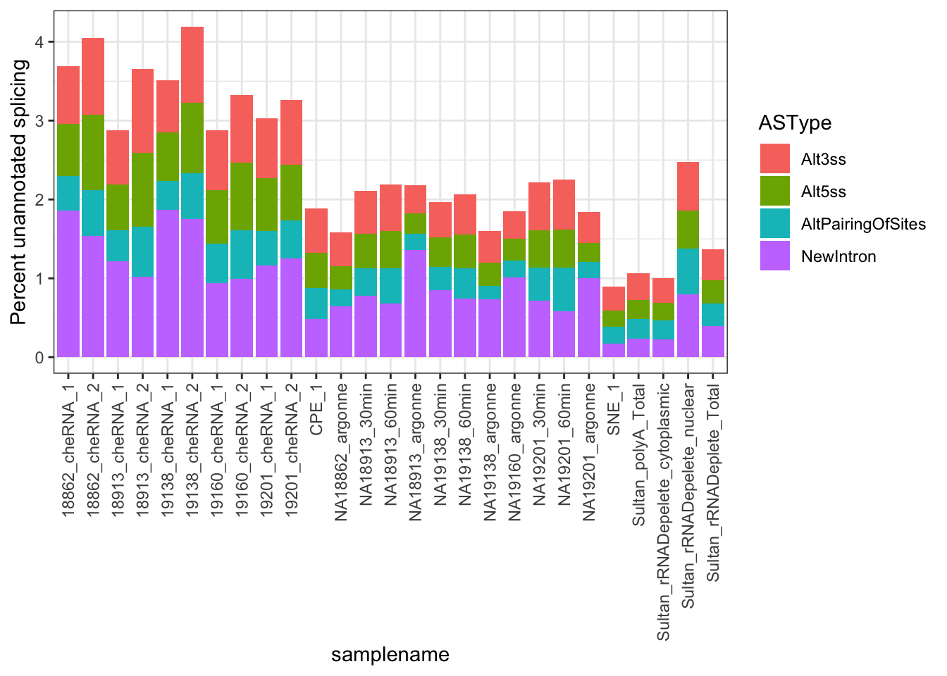
| Version | Author | Date |
|---|---|---|
| 9b62d8b | Benjmain Fair | 2019-08-26 |
#Same plot but plot percent NMD specific splicing
MergedData %>%
  mutate(Intron=paste(geneChr, start,stop,strand, sep=".")) %>%
  mutate(NMD.status = case_when(Intron %in% NMD.Specific.Introns ~ "NMD.Specific.Intron",
                                !Intron %in% NMD.Specific.Introns ~ "Not.NMD.Specific.Intron"
                                )) %>%
  group_by(samplename, NMD.status) %>%
  summarise(a_sum=sum(score)) %>%
  group_by(samplename) %>%
  mutate(FractionSpliceType = a_sum/sum(a_sum)*100) %>%
  filter(NMD.status=="NMD.Specific.Intron") %>%
  ggplot(aes(x = samplename, y = FractionSpliceType)) +
  geom_col() +
  ylab("Percent NMD.specific\njunction reads") +
  theme_bw() +
  theme(axis.text.x = element_text(angle = 90, hjust = 1, vjust=0.5))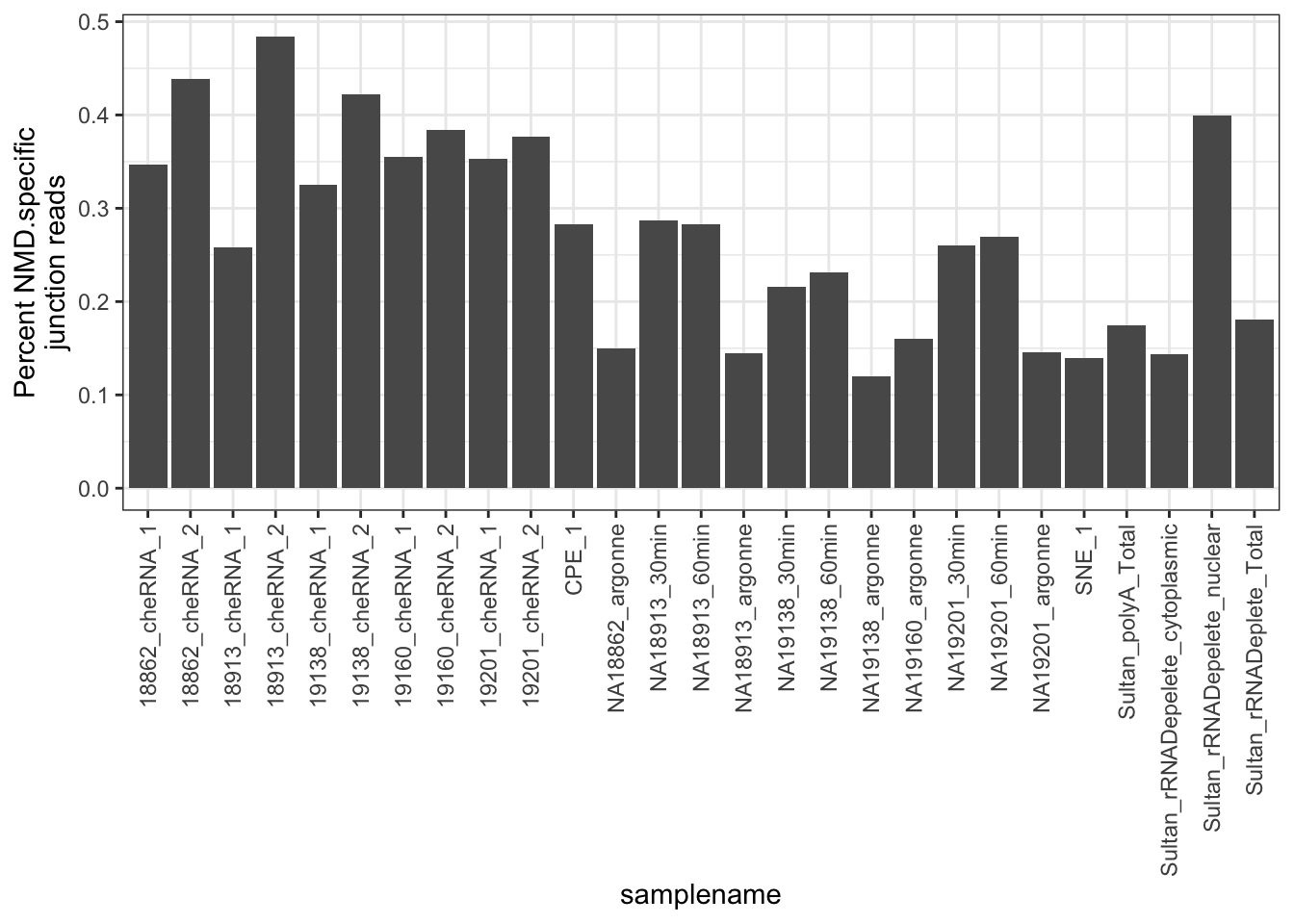
| Version | Author | Date |
|---|---|---|
| 9b62d8b | Benjmain Fair | 2019-08-26 |
#Same plot but count fraction of spliced reads as fraction of total mapped
TotalReadCounts <- read.table("../output/CountsPerBam.txt", header=T, sep='\t') %>%
  mutate(samplename = gsub(".+SecondPass/(.+?)/Aligned.sortedByCoord.+", "\\1", Filename, perl=T)) %>%
  select(samplename, ReadCount)

MergedData %>%
  group_by(samplename, ASType) %>%
  summarise(a_sum=sum(score)) %>%
  group_by(samplename) %>%
  left_join(TotalReadCounts) %>%
  mutate(FractionSpliceType = a_sum/ReadCount*100) %>%
  ggplot(aes(x = samplename, y = FractionSpliceType)) +
  geom_col() +
  ylab("Percent spliced reads") +
  theme_bw() +
  theme(axis.text.x = element_text(angle = 90, hjust = 1, vjust=0.5))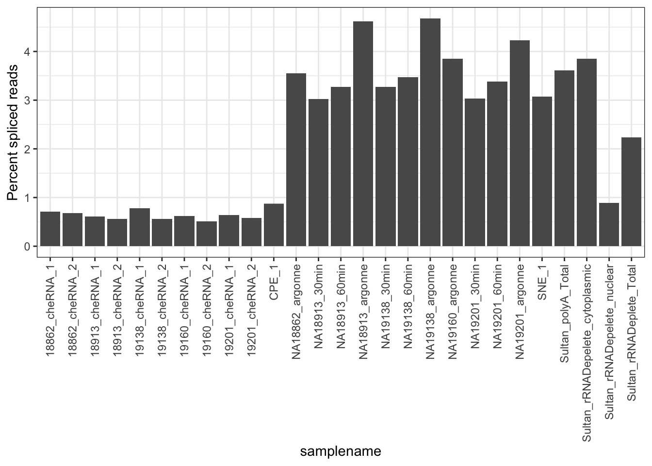
| Version | Author | Date |
|---|---|---|
| 9b62d8b | Benjmain Fair | 2019-08-26 |
#Where are called splice sites
MergedData %>%
  filter(samplename %in% SamplesToPlot) %>%
  filter(ASType!="AnnotatedSpliceSite") %>%
  filter(score>0) %>%
ggplot(aes(x=Rel3SplicePos, color=samplename)) +
  geom_density(adjust=2, size=1) +
  xlab("Relative position of unannotated splice site") +
  theme_bw()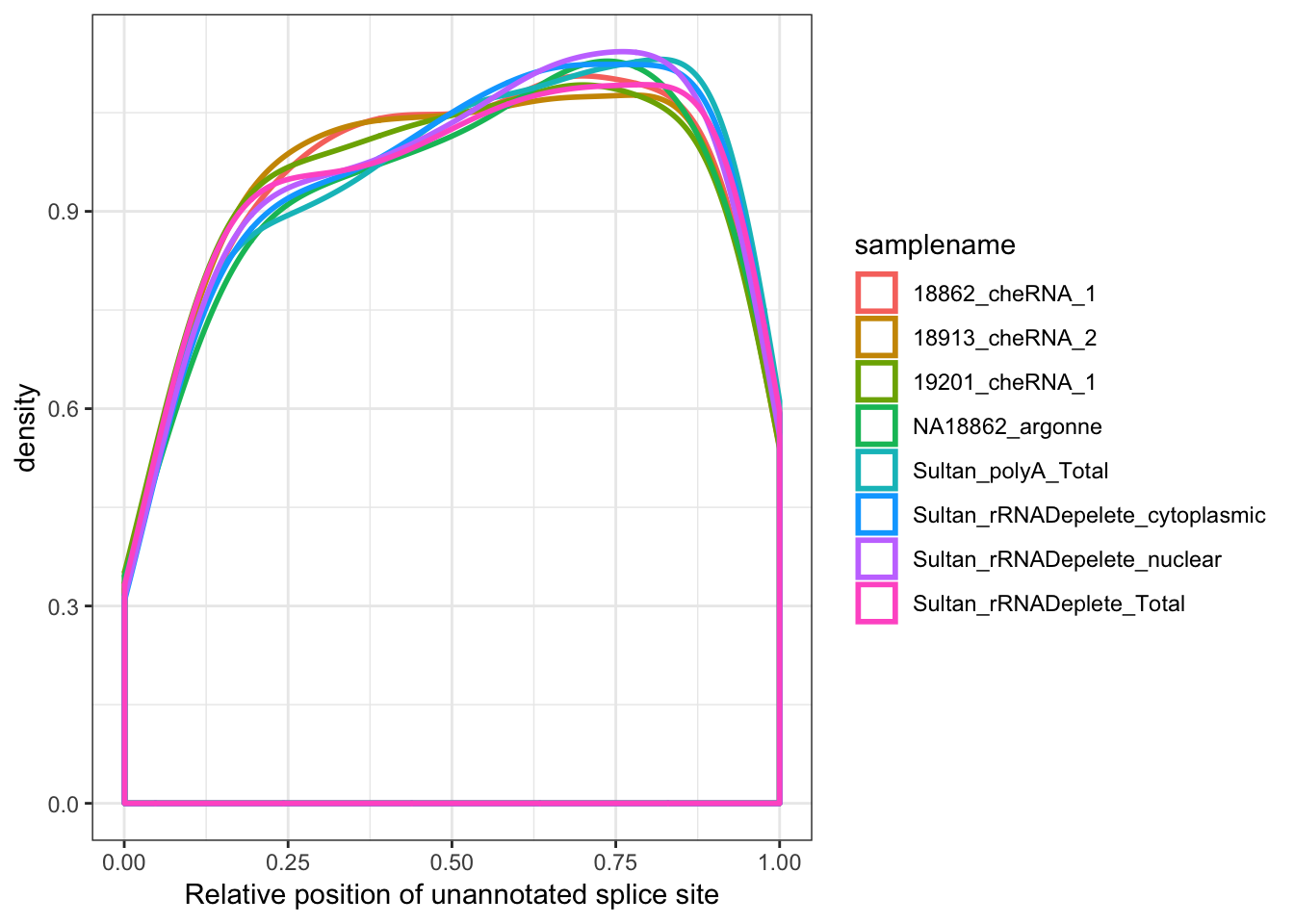
#Same, but weighted by RPM for junction, filtering out extreme outliers (>10 counts)
MergedData %>%
  filter(samplename %in% SamplesToPlot) %>%
  filter(ASType!="AnnotatedSpliceSite") %>%
  filter(score>0) %>%
  filter(score<10) %>%
  group_by(samplename) %>%
  mutate(a_sum=sum(score)) %>%
  ungroup() %>%
ggplot(aes(x=Rel5SplicePos, color=samplename)) +
  geom_density(adjust=2, aes(weight=score/a_sum)) +
  theme_bw()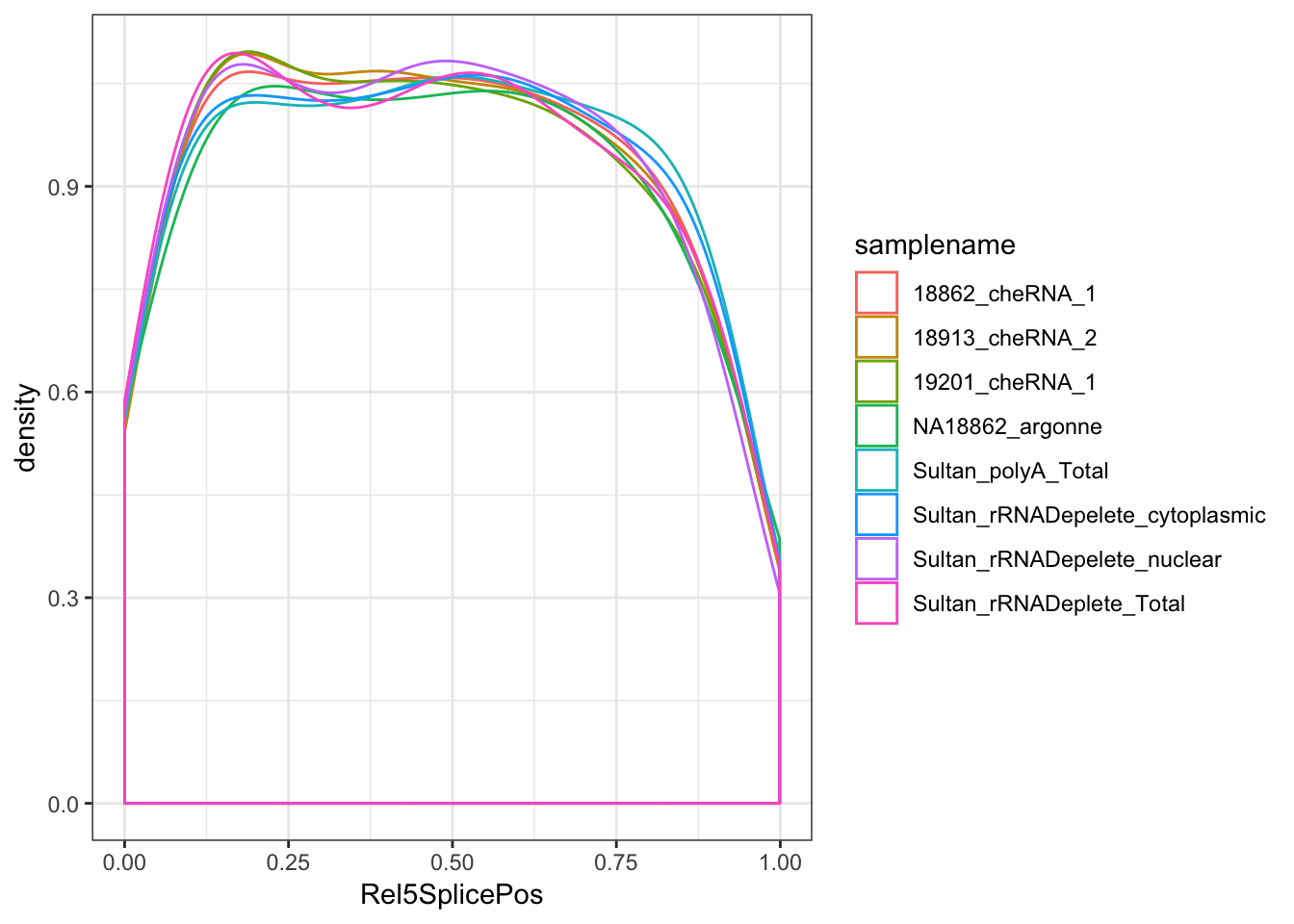
# MergedData %>%
#   filter(samplename %in% SamplesToPlot) %>%
#   filter(ASType!="AnnotatedSpliceSite") %>%
#   filter(score>0) %>%
#   group_by(samplename) %>%
#   mutate(a_sum=sum(score)) %>%
#   mutate(frac=score/a_sum)%>%
#   summarise(max=max(frac))
Ok, so nuclear (and chromatin associated) fractions have more unannotated splicing by a factor of about 1.5X to 2X, and of those unannotated splice sites seem very slightly biased towards the 5’ end of genes.
As a control, I should make the same metaplots for annotated splice sites
#Where are splice events
MergedData %>%
  filter(samplename %in% SamplesToPlot) %>%
  filter(ASType=="AnnotatedSpliceSite") %>%
  filter(score>0) %>%
  ggplot(aes(x=Rel3SplicePos, color=samplename)) +
    geom_density(adjust=2, size=1) +
    xlab("Relative position of annotated splice site") +
    theme_bw()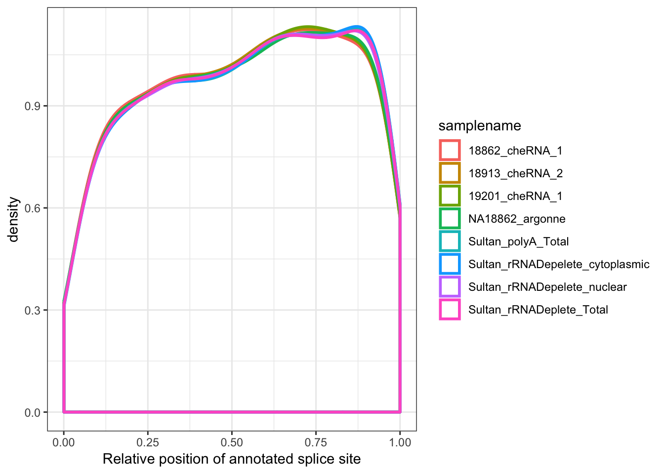
| Version | Author | Date |
|---|---|---|
| 9b62d8b | Benjmain Fair | 2019-08-26 |
#Same but weighted by junction RPM
ToPlot <- MergedData %>%
  filter(samplename %in% SamplesToPlot) %>%
  filter(ASType=="AnnotatedSpliceSite") %>%
  filter(score>0) %>%
  filter(score<500) %>%
  group_by(samplename) %>%
  mutate(a_sum=sum(score)) %>%
  ungroup()
ggplot(ToPlot, aes(x=Rel3SplicePos, color=samplename)) +
  geom_density(adjust=2, size=1, aes(weight=score/a_sum)) +
  theme_bw()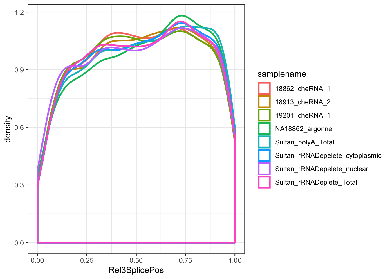
| Version | Author | Date |
|---|---|---|
| 9b62d8b | Benjmain Fair | 2019-08-26 |
MergedData %>%
  filter(samplename %in% SamplesToPlot) %>%
  filter(ASType=="AnnotatedSpliceSite") %>%
  filter(score>0) %>%
ggplot(aes(x=log10(score), color=samplename)) +
  geom_density() +
  theme_bw()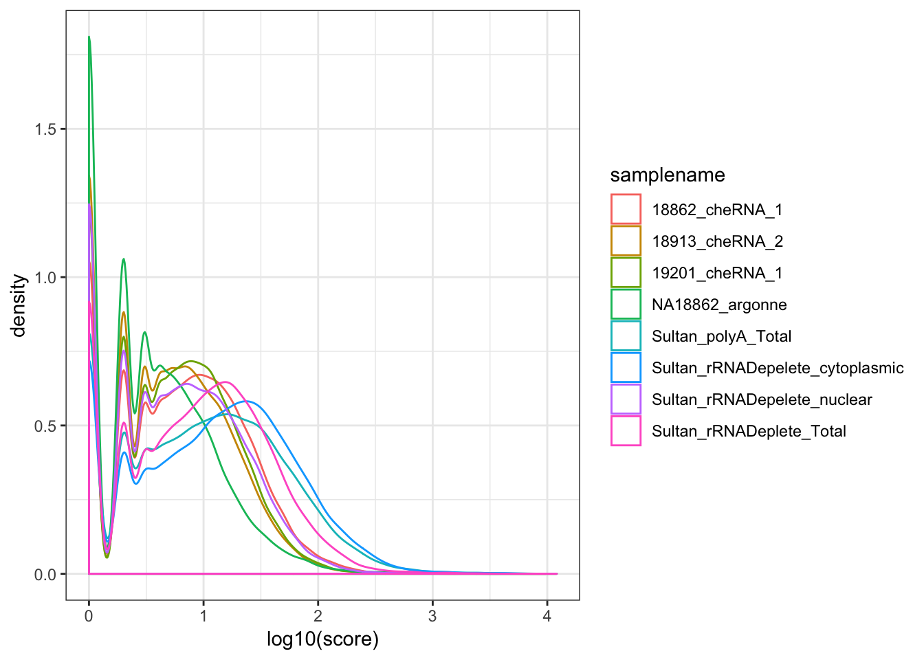
Ok, good. So the 5’ enrichment for splice sites in chromatin-associated RNAs is true for unannotated splice sites but not for annotated splice sites.
Ok finally, to complement the idea that this 5’ enrichment of novel splice sites has something to do with NMD decay of alternative transcripts, make some metagene plots of positions of introns that are Genocde annotated as within NMD target transcripts.
MergedData %>%
  mutate(Intron=paste(geneChr, start,stop,strand, sep=".")) %>%
  mutate(NMD.status = case_when(Intron %in% NMD.Specific.Introns ~ "NMD.Specific.Intron",
                                !Intron %in% NMD.Specific.Introns ~ "Not.NMD.Specific.Intron"
                                )) %>%
  filter(samplename %in% SamplesToPlot) %>%
  filter(ASType=="AnnotatedSpliceSite") %>%
  filter(score<500) %>%
  group_by(samplename) %>%
  mutate(a_sum=sum(score)) %>%
  ungroup() %>%
ggplot(aes(x=Rel3SplicePos, color=samplename)) +
  geom_density(aes(linetype=NMD.status), adjust=2, size=1) +
  xlab("Relative position of splice site") +
  theme_bw()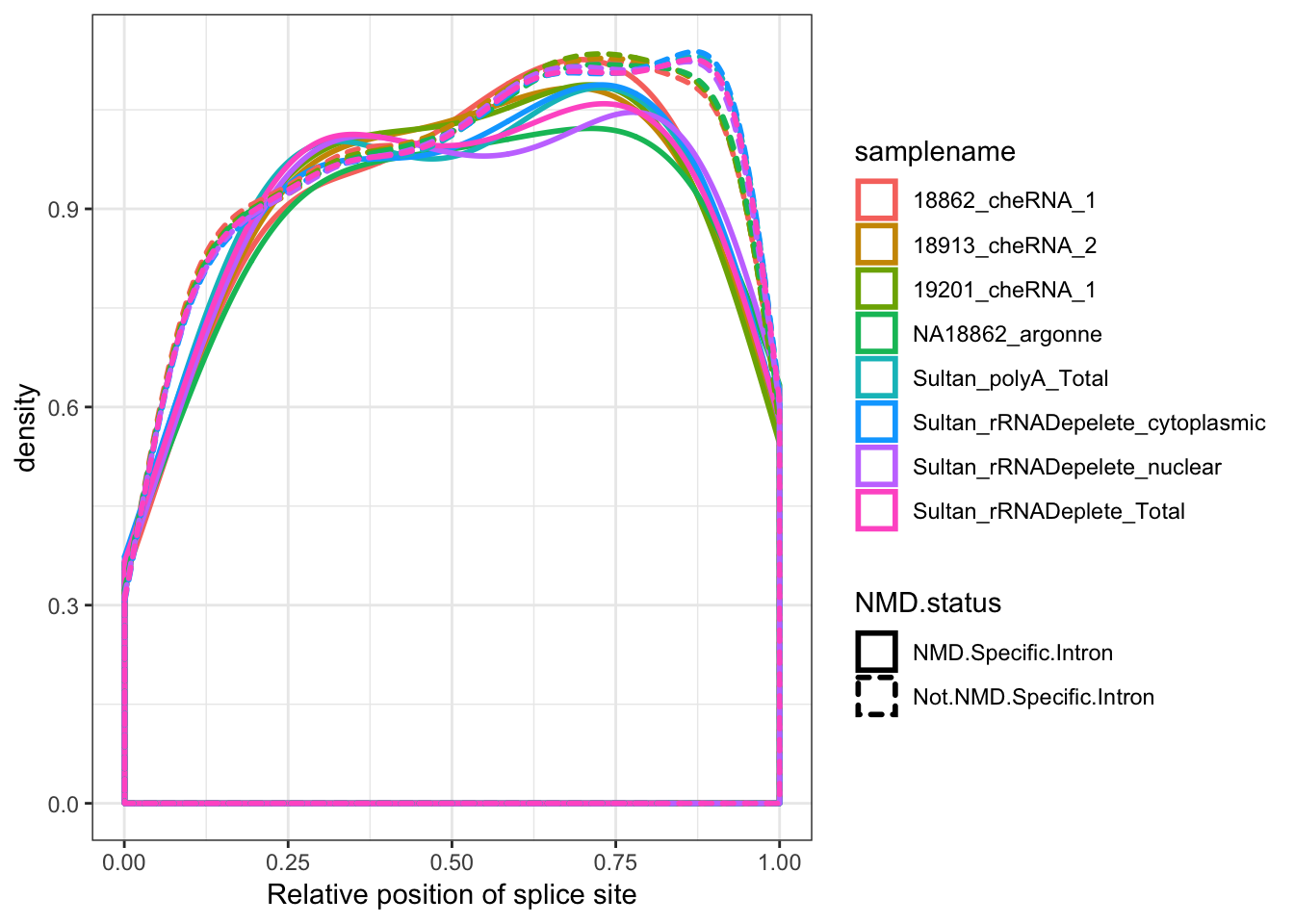
sessionInfo()R version 3.5.1 (2018-07-02)
Platform: x86_64-apple-darwin15.6.0 (64-bit)
Running under: macOS 10.14
Matrix products: default
BLAS: /Library/Frameworks/R.framework/Versions/3.5/Resources/lib/libRblas.0.dylib
LAPACK: /Library/Frameworks/R.framework/Versions/3.5/Resources/lib/libRlapack.dylib
locale:
[1] en_US.UTF-8/en_US.UTF-8/en_US.UTF-8/C/en_US.UTF-8/en_US.UTF-8
attached base packages:
[1] stats graphics grDevices utils datasets methods base
other attached packages:
[1] forcats_0.4.0 stringr_1.4.0 dplyr_0.8.1 purrr_0.3.2
[5] readr_1.3.1 tidyr_0.8.3 tibble_2.1.3 ggplot2_3.1.1
[9] tidyverse_1.2.1
loaded via a namespace (and not attached):
[1] Rcpp_1.0.1 cellranger_1.1.0 plyr_1.8.4 pillar_1.4.1
[5] compiler_3.5.1 git2r_0.25.2 workflowr_1.4.0 tools_3.5.1
[9] digest_0.6.19 lubridate_1.7.4 jsonlite_1.6 evaluate_0.14
[13] nlme_3.1-140 gtable_0.3.0 lattice_0.20-38 pkgconfig_2.0.2
[17] rlang_0.3.4 cli_1.1.0 rstudioapi_0.10 yaml_2.2.0
[21] haven_2.1.0 xfun_0.7 withr_2.1.2 xml2_1.2.0
[25] httr_1.4.0 knitr_1.23 hms_0.4.2 generics_0.0.2
[29] fs_1.3.1 rprojroot_1.3-2 grid_3.5.1 tidyselect_0.2.5
[33] glue_1.3.1 R6_2.4.0 readxl_1.3.1 rmarkdown_1.13
[37] modelr_0.1.4 magrittr_1.5 whisker_0.3-2 backports_1.1.4
[41] scales_1.0.0 htmltools_0.3.6 rvest_0.3.4 assertthat_0.2.1
[45] colorspace_1.4-1 labeling_0.3 stringi_1.4.3 lazyeval_0.2.2
[49] munsell_0.5.0 broom_0.5.2 crayon_1.3.4