20190909_Count3ssRatioExample
Ben Fair
9/10/2019
Last updated: 2019-09-16
Checks: 6 1
Knit directory: cheRNA_pilot/analysis/
This reproducible R Markdown analysis was created with workflowr (version 1.4.0). The Checks tab describes the reproducibility checks that were applied when the results were created. The Past versions tab lists the development history.
The R Markdown is untracked by Git. To know which version of the R Markdown file created these results, you’ll want to first commit it to the Git repo. If you’re still working on the analysis, you can ignore this warning. When you’re finished, you can run wflow_publish to commit the R Markdown file and build the HTML.
Great job! The global environment was empty. Objects defined in the global environment can affect the analysis in your R Markdown file in unknown ways. For reproduciblity it’s best to always run the code in an empty environment.
The command set.seed(20190813) was run prior to running the code in the R Markdown file. Setting a seed ensures that any results that rely on randomness, e.g. subsampling or permutations, are reproducible.
Great job! Recording the operating system, R version, and package versions is critical for reproducibility.
Nice! There were no cached chunks for this analysis, so you can be confident that you successfully produced the results during this run.
Great job! Using relative paths to the files within your workflowr project makes it easier to run your code on other machines.
Great! You are using Git for version control. Tracking code development and connecting the code version to the results is critical for reproducibility. The version displayed above was the version of the Git repository at the time these results were generated.
Note that you need to be careful to ensure that all relevant files for the analysis have been committed to Git prior to generating the results (you can use wflow_publish or wflow_git_commit). workflowr only checks the R Markdown file, but you know if there are other scripts or data files that it depends on. Below is the status of the Git repository when the results were generated:
Ignored files:
    Ignored:    .Rhistory
    Ignored:    .Rproj.user/

Untracked files:
    Untracked:  analysis/20190909_Count3ssRatioExample.Rmd

Unstaged changes:
    Modified:   analysis/20190805_PlotIntronPositions.Rmd
Note that any generated files, e.g. HTML, png, CSS, etc., are not included in this status report because it is ok for generated content to have uncommitted changes.
There are no past versions. Publish this analysis with wflow_publish() to start tracking its development.
library(tidyverse)For each 3’ss, I used bedtools to count the number of reads overlapping the upstream 25bp window, and the downstream 25bp window. The ratio of these of these two counts is a measure of splicing efficiency, and the ratio of those ratios in nascent RNA-seq versus standard RNA-seq is a measure of how contranscriptional a splicing event is (see Herzel et al). Here I will look at these metrics using a standard RNA-seq dataset and nascent RNA-seq dataset from the same LCL line 18862.
I have already calculated counts in upstream and downstream windows for each annotated 3’ss using bedtools (see Snakemake code). Here I will investigate the results with a few plots. One result I expect to see is that alernative 3’ss will be spliced less contranscripionally. In the case of cassette exons, it is important to distinguish between the upstream 3’ss and the downstream 3’ss.
First read in Gencode annotated introns, and classif the 3’ss as alternative or constitutive.
GencodeIntrons <- read.table("../data/GencodeHg38_all_introns.corrected.bed.gz", sep='\t', col.names = c('chrom', 'start', 'stop', 'name', 'score', 'strand', 'gene', 'intronNumber', 'transcriptType'))

SpliceSitesCounted <- GencodeIntrons %>%
  filter(transcriptType=="protein_coding") %>%
  distinct(chrom, start, stop, .keep_all = T) %>%
  mutate(Acceptor = case_when(strand == "+" ~ paste(chrom, stop, strand, sep="."),
                              strand == "-" ~ paste(chrom, start, strand, sep="."))) %>%
  mutate(Donor = case_when(strand == "+" ~ paste(chrom, start, strand, sep="."),
                           strand == "-" ~ paste(chrom, stop, strand, sep="."))) %>%
  add_count(Acceptor, name="AcceptorCount") %>%
  add_count(Donor, name="DonorCount")

Annotated <- SpliceSitesCounted %>%
  # filter(AcceptorCount==1 & DonorCount==1) %>% dim()
  group_by(Acceptor) %>%
  mutate(DonorMax=max(DonorCount)) %>%
  ungroup() %>%
  distinct(Acceptor, .keep_all = T) %>%
  mutate(Type3ss = case_when(AcceptorCount == 1 & DonorMax==1 ~ "Constitutive intron",
                             AcceptorCount >1 & DonorMax==1 ~ "Downstream alternative intron",
                             DonorMax > 1 ~ "Upstream alternative intron"))

table(Annotated$Type3ss)
          Constitutive intron Downstream alternative intron
                       149839                          7003
  Upstream alternative intron
                        51850
Annotated %>%
mutate(NewName=paste(Acceptor, Type3ss, sep=".")) %>%
# mutate(NewStart = case_when(strand == "+" ~ stop-25,
# strand == "-" ~ start)) %>%
# mutate(NewStop = case_when(strand == "+" ~ stop,
# strand == "-" ~ start-25)) %>%
# select(chrom, NewStart, NewStop, paste(Acceptor, Type3ss), ".", strand) %>% head()
select(chrom, start, stop, NewName, score, strand) %>%
write.table("~/Temporary/3ssAnnotations.bed", quote=F, sep='\t', col.names=F, row.names = F)Now, similarly to Herzel et al, set a minimum read count threshold cutoff for reliable 3’ss splice ratios to use for downstream analysis. Then do some plotting.
Cutoff <- 50

RS <- read.table("../output/3ssCoverageBeds/NA18862_argonne.bed.gz", sep='\t', col.names = c('chrom', 'start', 'stop', 'name', 'score', 'strand', 'upstream', 'downstream'), stringsAsFactors = F) %>% filter(upstream + downstream >= Cutoff)
nRS <- read.table("../output/3ssCoverageBeds/18862_cheRNA_1.bed.gz", sep='\t', col.names = c('chrom', 'start', 'stop', 'name', 'score', 'strand', 'upstream', 'downstream'), stringsAsFactors = F) %>% filter(upstream + downstream >= Cutoff)

ToPlot <- RS %>%
  left_join(nRS, by="name") %>%
  inner_join(Annotated, by=c("name" = "Acceptor"))%>%
  mutate(RS.ratio = upstream.x/(downstream.x+upstream.x)) %>%
  mutate(nRS.ratio = upstream.y/(downstream.y+upstream.y)) %>%
  mutate(NormalizedRatio = nRS.ratio/RS.ratio)

ggplot(ToPlot, aes(color=Type3ss)) +
  stat_ecdf(aes(x=nRS.ratio, linetype="nascent-RNA"), geom = "step") +
  stat_ecdf(aes(x=RS.ratio, linetype="polyA-RNA"), geom = "step") +
  ylab('Cumulative fraction') +
  xlab("Intron retention PSI") +
  theme_bw()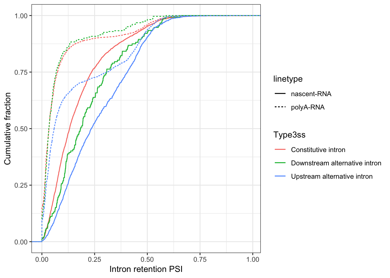
ggplot(ToPlot, aes(x=NormalizedRatio, color=Type3ss)) +
  stat_ecdf(geom = "step") +
  ylab('Cumulative fraction') +
  xlab("Cotranscriptional splicing ratio") +
  theme_bw()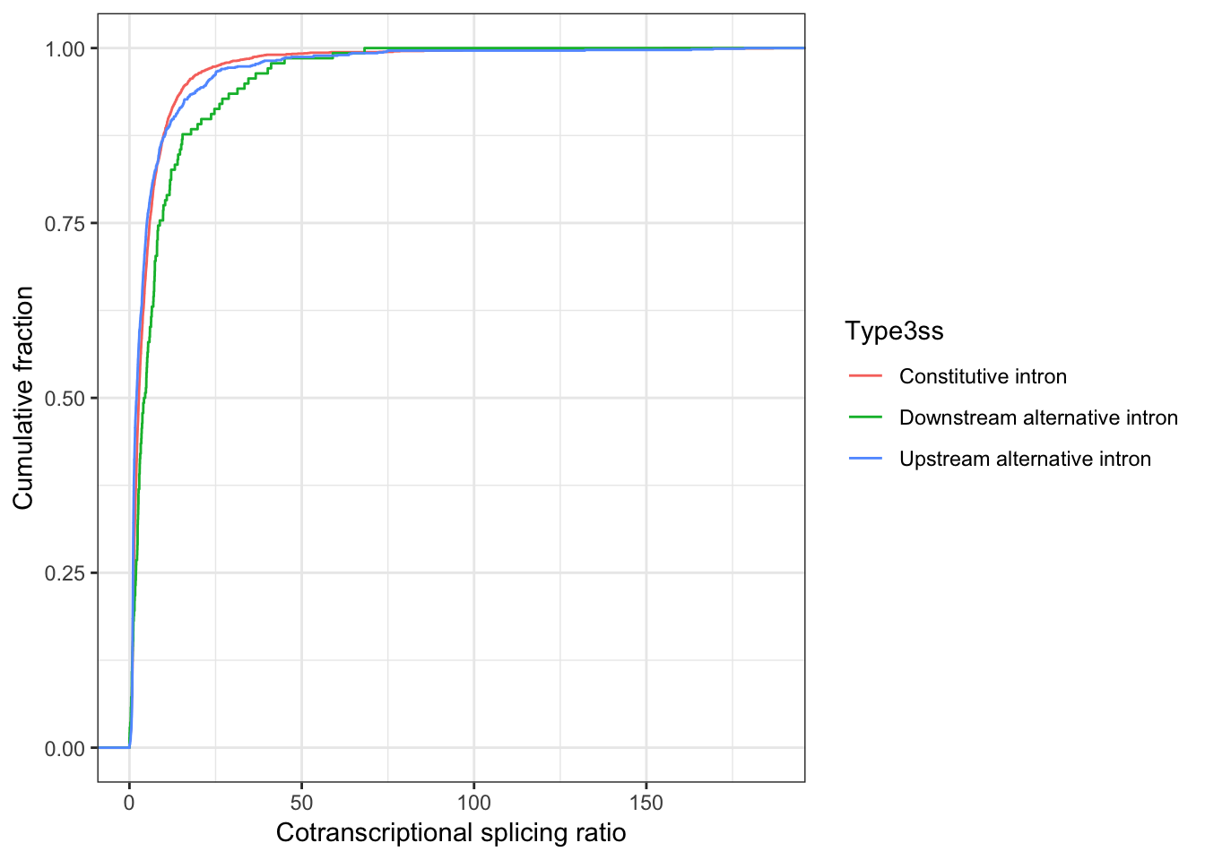
ToTest <- ToPlot %>%
  filter(Type3ss %in% c("Constitutive intron", "Downstream alternative intron"))
wilcox.test(NormalizedRatio ~ Type3ss, data=ToTest)
    Wilcoxon rank sum test with continuity correction

data:  NormalizedRatio by Type3ss
W = 134980, p-value = 0.0002172
alternative hypothesis: true location shift is not equal to 0
sessionInfo()R version 3.5.1 (2018-07-02)
Platform: x86_64-apple-darwin15.6.0 (64-bit)
Running under: macOS 10.14
Matrix products: default
BLAS: /Library/Frameworks/R.framework/Versions/3.5/Resources/lib/libRblas.0.dylib
LAPACK: /Library/Frameworks/R.framework/Versions/3.5/Resources/lib/libRlapack.dylib
locale:
[1] en_US.UTF-8/en_US.UTF-8/en_US.UTF-8/C/en_US.UTF-8/en_US.UTF-8
attached base packages:
[1] stats graphics grDevices utils datasets methods base
other attached packages:
[1] forcats_0.4.0 stringr_1.4.0 dplyr_0.8.1 purrr_0.3.2
[5] readr_1.3.1 tidyr_0.8.3 tibble_2.1.3 ggplot2_3.1.1
[9] tidyverse_1.2.1
loaded via a namespace (and not attached):
[1] Rcpp_1.0.1 cellranger_1.1.0 plyr_1.8.4 pillar_1.4.1
[5] compiler_3.5.1 git2r_0.25.2 workflowr_1.4.0 tools_3.5.1
[9] digest_0.6.19 lubridate_1.7.4 jsonlite_1.6 evaluate_0.14
[13] nlme_3.1-140 gtable_0.3.0 lattice_0.20-38 pkgconfig_2.0.2
[17] rlang_0.3.4 cli_1.1.0 rstudioapi_0.10 yaml_2.2.0
[21] haven_2.1.0 xfun_0.7 withr_2.1.2 xml2_1.2.0
[25] httr_1.4.0 knitr_1.23 hms_0.4.2 generics_0.0.2
[29] fs_1.3.1 rprojroot_1.3-2 grid_3.5.1 tidyselect_0.2.5
[33] glue_1.3.1 R6_2.4.0 readxl_1.3.1 rmarkdown_1.13
[37] modelr_0.1.4 magrittr_1.5 backports_1.1.4 scales_1.0.0
[41] htmltools_0.3.6 rvest_0.3.4 assertthat_0.2.1 colorspace_1.4-1
[45] labeling_0.3 stringi_1.4.3 lazyeval_0.2.2 munsell_0.5.0
[49] broom_0.5.2 crayon_1.3.4