Data integration and clustering of cardiomyocytes: fetal, young, adult

workflowr

• Summary
• Checks
• Past versions

Last updated: 2019-10-21

Checks: 6 0

Knit directory: Porello-heart-snRNAseq/

This reproducible R Markdown analysis was created with workflowr (version 1.3.0). The Checks tab describes the reproducibility checks that were applied when the results were created. The Past versions tab lists the development history.

---

R Markdown file: up-to-date

Great! Since the R Markdown file has been committed to the Git repository, you know the exact version of the code that produced these results.

Environment: empty

Great job! The global environment was empty. Objects defined in the global environment can affect the analysis in your R Markdown file in unknown ways. For reproduciblity it’s best to always run the code in an empty environment.

Seed: set.seed(20190603)

The command set.seed(20190603) was run prior to running the code in the R Markdown file. Setting a seed ensures that any results that rely on randomness, e.g. subsampling or permutations, are reproducible.

Session information: recorded

Great job! Recording the operating system, R version, and package versions is critical for reproducibility.

Cache: none

Nice! There were no cached chunks for this analysis, so you can be confident that you successfully produced the results during this run.

Repository version: 6c4e378

Great! You are using Git for version control. Tracking code development and connecting the code version to the results is critical for reproducibility. The version displayed above was the version of the Git repository at the time these results were generated.

Note that you need to be careful to ensure that all relevant files for the analysis have been committed to Git prior to generating the results (you can use wflow_publish or wflow_git_commit). workflowr only checks the R Markdown file, but you know if there are other scripts or data files that it depends on. Below is the status of the Git repository when the results were generated:

Ignored files:
    Ignored:    .Rhistory
    Ignored:    .Rproj.user/

Untracked files:
    Untracked:  analysis/08-ClustEpicardial.Rmd
    Untracked:  analysis/PBapproachMarker-cardio.Rmd
    Untracked:  analysis/doublet-detection.Rmd
    Untracked:  broad_props.csv
    Untracked:  code/ReadDataObjects.R
    Untracked:  code/getTransformedProps.R
    Untracked:  data/adult-clust.txt
    Untracked:  data/dcm-clust.txt
    Untracked:  data/fetal-clust.txt
    Untracked:  data/gstlist-adult.Rdata
    Untracked:  data/gstlist-dcm-res03.Rdata
    Untracked:  data/gstlist-dcm.Rdata
    Untracked:  data/gstlist-fetal.Rdata
    Untracked:  data/gstlist-young.Rdata
    Untracked:  data/heart-markers-long.txt
    Untracked:  data/immune-markers-long.txt
    Untracked:  data/pseudobulk-pool.Rds
    Untracked:  data/pseudobulk.Rds
    Untracked:  data/targets_pools.txt
    Untracked:  data/young-clust.txt
    Untracked:  output/AllAdult-clustermarkers-v2.csv
    Untracked:  output/AllAdult-clustermarkers.csv
    Untracked:  output/AllFetal-clustermarkers.csv
    Untracked:  output/AllYoung-clustermarkers.csv
    Untracked:  output/Alldcm-clustermarkers.csv
    Untracked:  output/DEAnalysis/
    Untracked:  output/Figures/
    Untracked:  output/MarkerAnalysis/
    Untracked:  output/RDataObjects/
    Untracked:  output/cardio-numcells-clusters.csv
    Untracked:  output/cardio-numcells-clusters.txt
    Untracked:  output/fetal1-clustermarkers.csv
    Untracked:  output/fetal2-clustermarkers.csv
    Untracked:  output/fetal3-clustermarkers.csv
    Untracked:  output/heatmap-top10-adultmarkergenes.pdf
    Untracked:  output/young1-clustermarkers.csv

Unstaged changes:
    Modified:   analysis/01-QualityControl.Rmd
    Modified:   analysis/01a-DEpseudobulk.Rmd
    Modified:   analysis/02-ClusterFetal.Rmd
    Modified:   analysis/02c-ClusterFetal3.Rmd
    Modified:   analysis/03-ClusterYoung.Rmd
    Modified:   analysis/04-ClusterAdult.Rmd
    Modified:   analysis/07b-DECardio.Rmd

Note that any generated files, e.g. HTML, png, CSS, etc., are not included in this status report because it is ok for generated content to have uncommitted changes.

---

These are the previous versions of the R Markdown and HTML files. If you’ve configured a remote Git repository (see ?wflow_git_remote), click on the hyperlinks in the table below to view them.

File	Version	Author	Date	Message
Rmd	6c4e378	Belinda Phipson	2019-10-21	update cardiomyocyte clustering with filtered data
html	67c1d63	Belinda Phipson	2019-10-18	Build site.
Rmd	eaa7f38	Belinda Phipson	2019-10-18	clustering of development samples

---

Load libraries and functions

library(edgeR)
library(RColorBrewer)
library(org.Hs.eg.db)
library(limma)
library(Seurat)
library(monocle)
library(cowplot)
library(DelayedArray)
library(scran)
library(NMF)
library(workflowr)
library(ggplot2)
library(clustree)
library(dplyr)

source("/misc/card2-single_cell_nuclei_rnaseq/Porello-heart-snRNAseq/code/normCounts.R")
source("/misc/card2-single_cell_nuclei_rnaseq/Porello-heart-snRNAseq/code/findModes.R")
source("/misc/card2-single_cell_nuclei_rnaseq/Porello-heart-snRNAseq/code/ggplotColors.R")

targets <- read.delim("/misc/card2-single_cell_nuclei_rnaseq/Porello-heart-snRNAseq/data/targets.txt",header=TRUE, stringsAsFactors = FALSE)
targets$FileName2 <- paste(targets$FileName,"/",sep="")
targets$Group_ID2 <- gsub("LV_","",targets$Group_ID)
group <- c("Fetal_1","Fetal_2","Fetal_3",
           "Young_1","Young_2","Young_3",
           "Adult_1","Adult_2","Adult_3", 
           "Diseased_1","Diseased_2",
           "Diseased_3","Diseased_4")
m <- match(group, targets$Group_ID2)
targets <- targets[m,]

fetal.integrated <- readRDS(file="./output/RDataObjects/fetal-int.Rds")
load(file="./output/RDataObjects/fetalObjs.Rdata")

young.integrated <- readRDS(file="./output/RDataObjects/young-int.Rds")
load(file="./output/RDataObjects/youngObjs.Rdata")

adult.integrated <- readRDS(file="./output/RDataObjects/adult-int.Rds")
load(file="./output/RDataObjects/adultObjs.Rdata")

Set default clustering resolution

# Default 0.3
Idents(fetal.integrated) <- fetal.integrated$integrated_snn_res.0.3
DimPlot(fetal.integrated, reduction = "tsne",label=TRUE,label.size = 6)+NoLegend()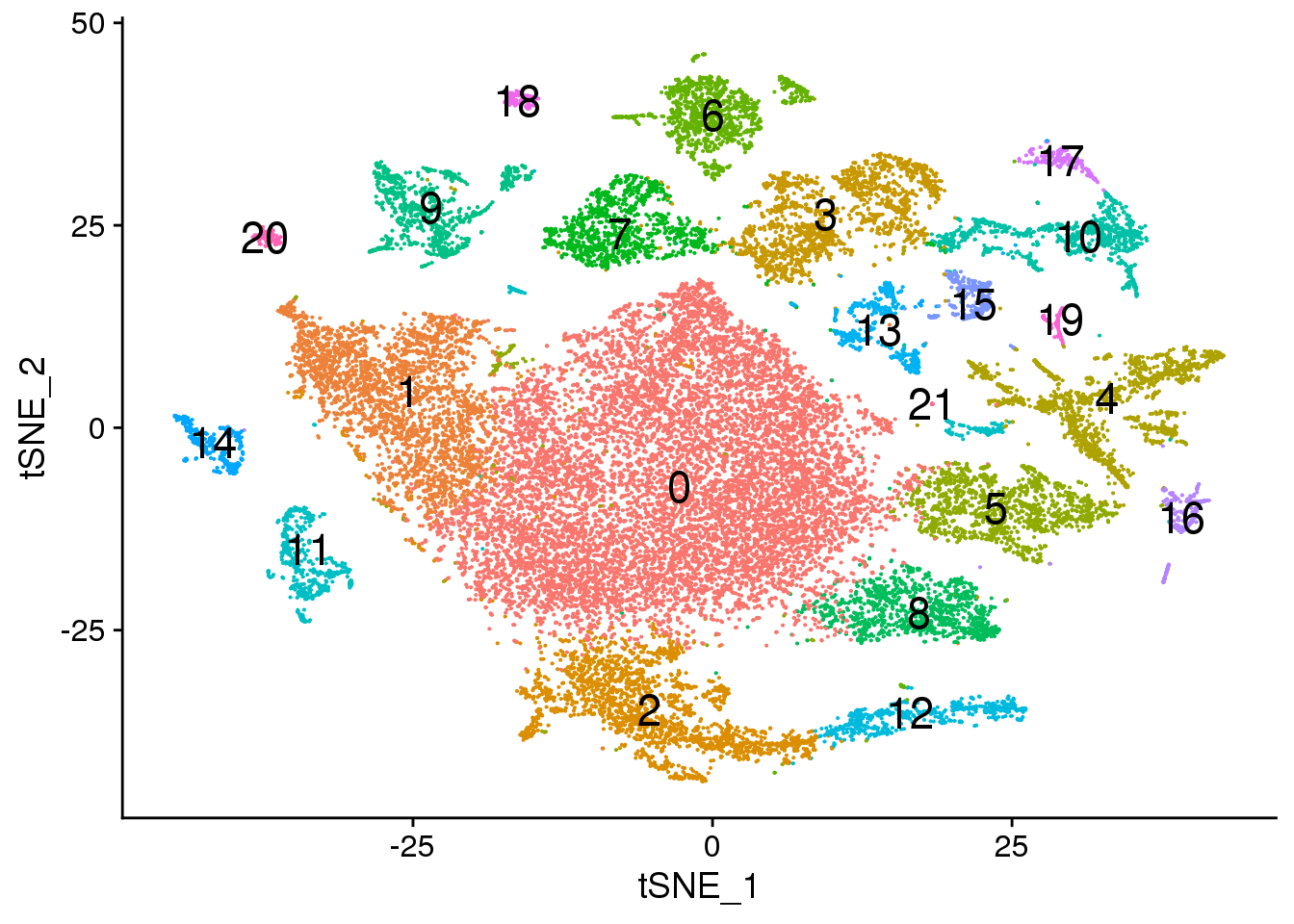

Past versions of unnamed-chunk-3-1.png

Version	Author	Date
67c1d63	Belinda Phipson	2019-10-18

# Default 0.3
DimPlot(young.integrated, reduction = "tsne",label=TRUE,label.size = 6)+NoLegend()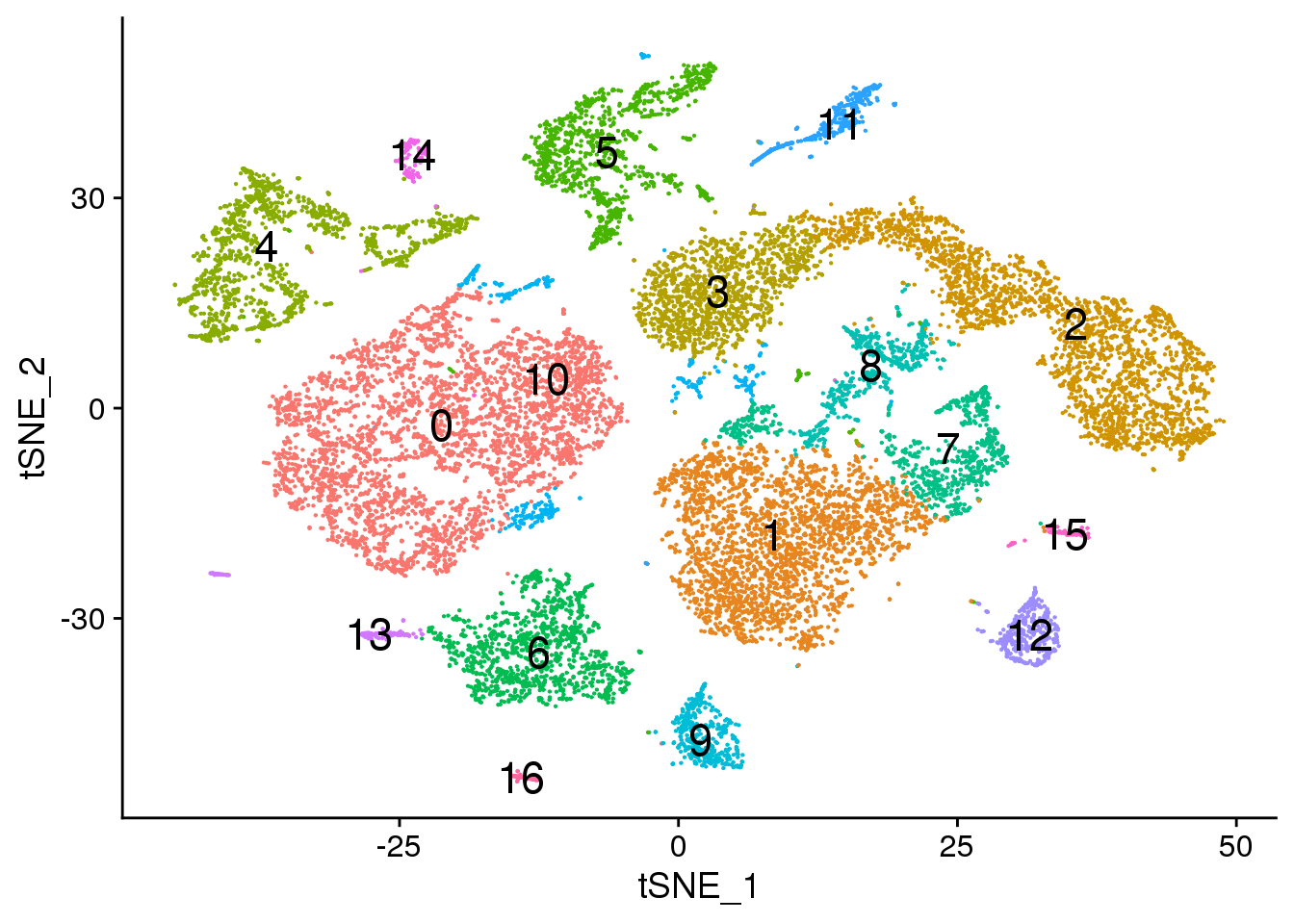

Past versions of unnamed-chunk-3-2.png

Version	Author	Date
67c1d63	Belinda Phipson	2019-10-18

# Default 0.6
DimPlot(adult.integrated, reduction = "tsne",label=TRUE,label.size = 6)+NoLegend()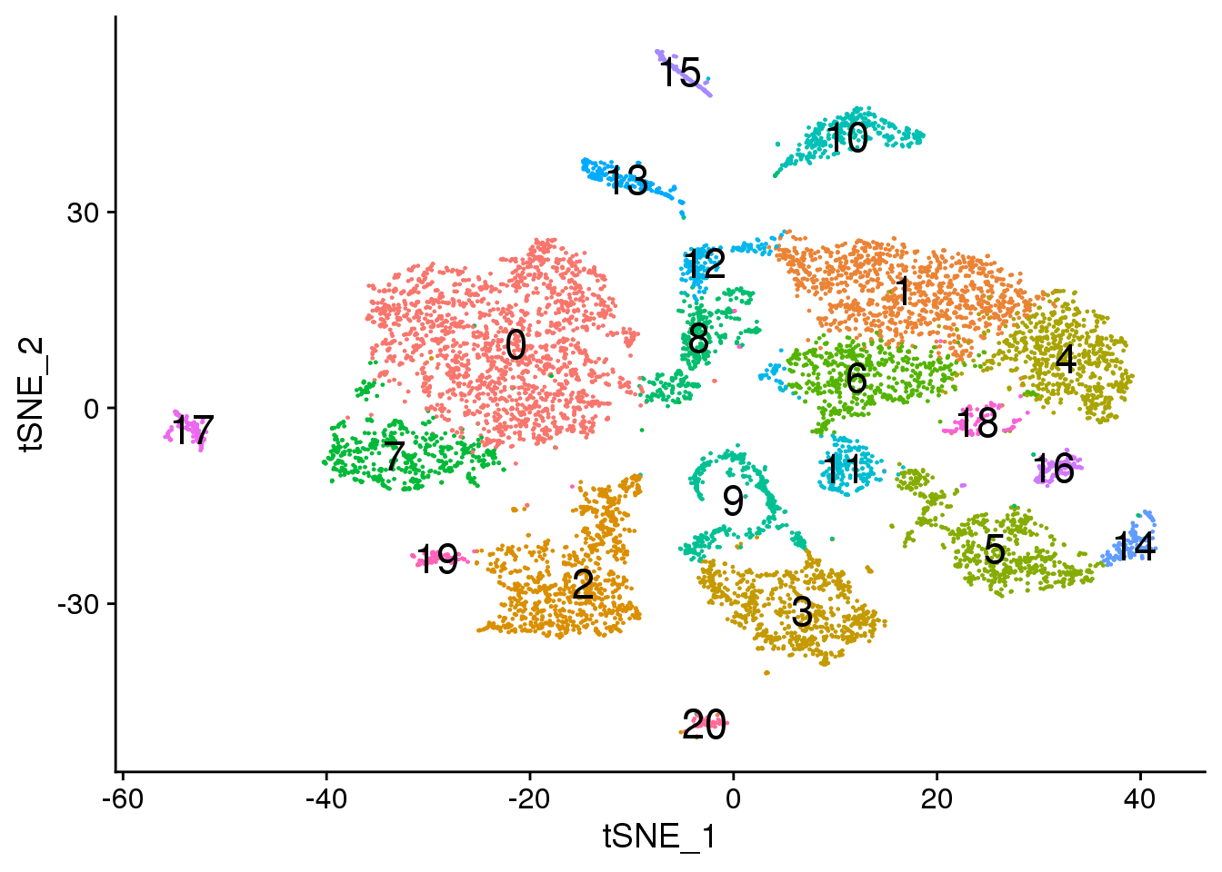

Past versions of unnamed-chunk-3-3.png

Version	Author	Date
67c1d63	Belinda Phipson	2019-10-18

Merge all data together

heart <- merge(fetal.integrated, y = c(young.integrated, adult.integrated), project = "heart")
table(heart$orig.ident)

adult fetal young 
 9416 27760 16964 

Get cardiomyocytes only

cardio <- subset(heart,subset = Broad_celltype == "Cardiomyocytes")

Filter out crappy cells

Cardiomyocytes are fairly large cells and we wouldn’t expect them to only be expressing very few genes.

par(mfrow=c(1,2))
plot(density(cardio$nFeature_RNA),main="Number of genes detected")
abline(v=500,col=2)
plot(density(cardio$nCount_RNA),main="Library size")
abline(v=2500,col=2)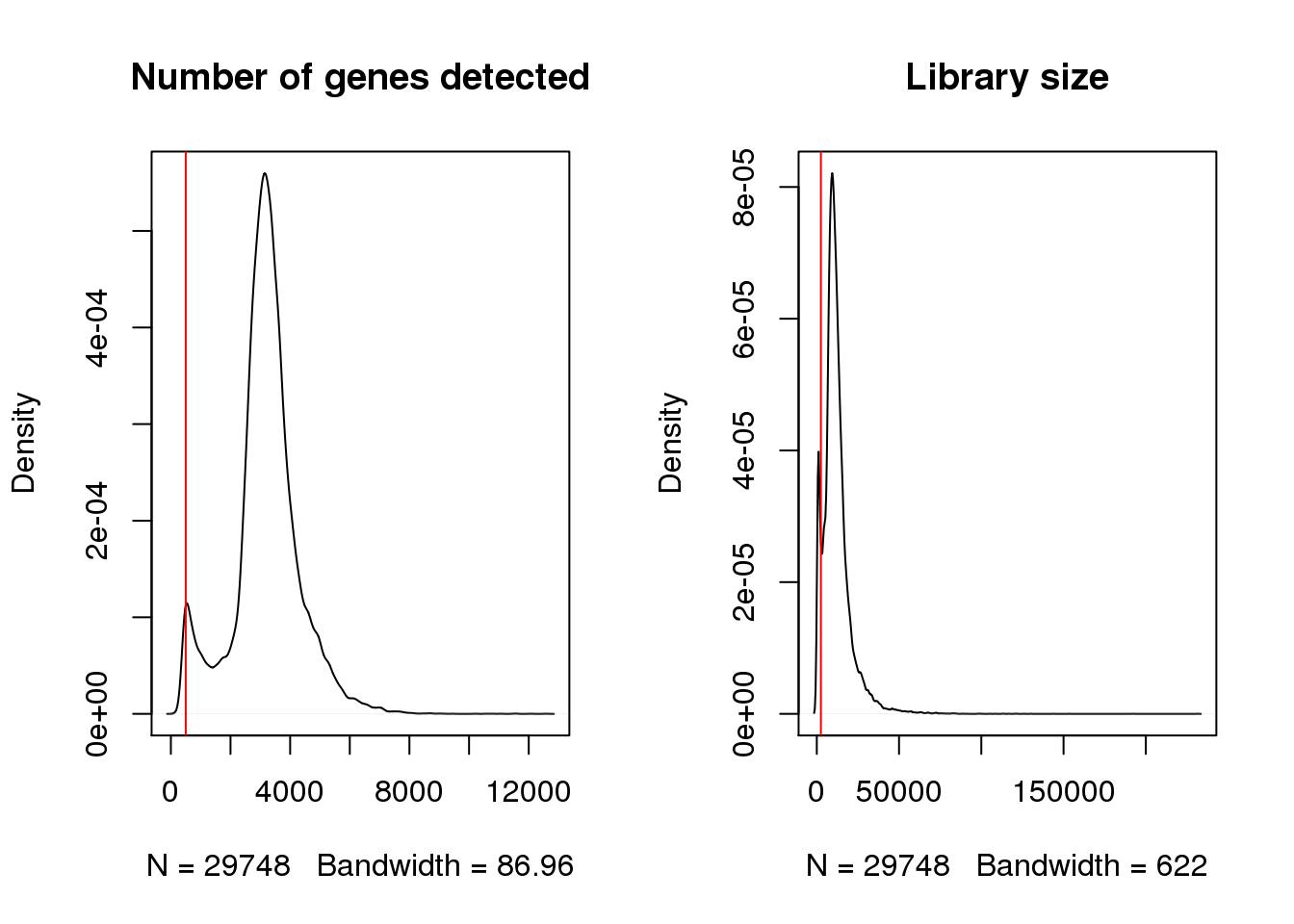

cardio <- subset(cardio, subset = nFeature_RNA > 500 & nCount_RNA > 2500)
dim(cardio)

[1]  4256 27037

table(cardio$biorep)

  a1   a2   a3   f1   f2   f3   y1   y2   y3 
1768  526  216 5435 8462 5114 1049 1962 2505 

Run new integration with SCtransform normalisation

The new code does not work so I will take the same approach that I took integrating the samples within groups.

cardio.list <- SplitObject(cardio, split.by = "biorep")
min(sapply(cardio.list, ncol))

[1] 216

for (i in 1:length(cardio.list)) {
    cardio.list[[i]] <- SCTransform(cardio.list[[i]], verbose = FALSE)
}

cardio.anchors <- FindIntegrationAnchors(object.list = cardio.list, dims=1:30,anchor.features = 3000,k.filter=216)

cardio.integrated <- IntegrateData(anchorset = cardio.anchors,dims=1:30)

Perform clustering

DefaultAssay(object = cardio.integrated) <- "integrated"

Perform scaling and PCA

cardio.integrated <- ScaleData(cardio.integrated, verbose = FALSE)
cardio.integrated <- RunPCA(cardio.integrated, npcs = 50, verbose = FALSE)
ElbowPlot(cardio.integrated,ndims=50)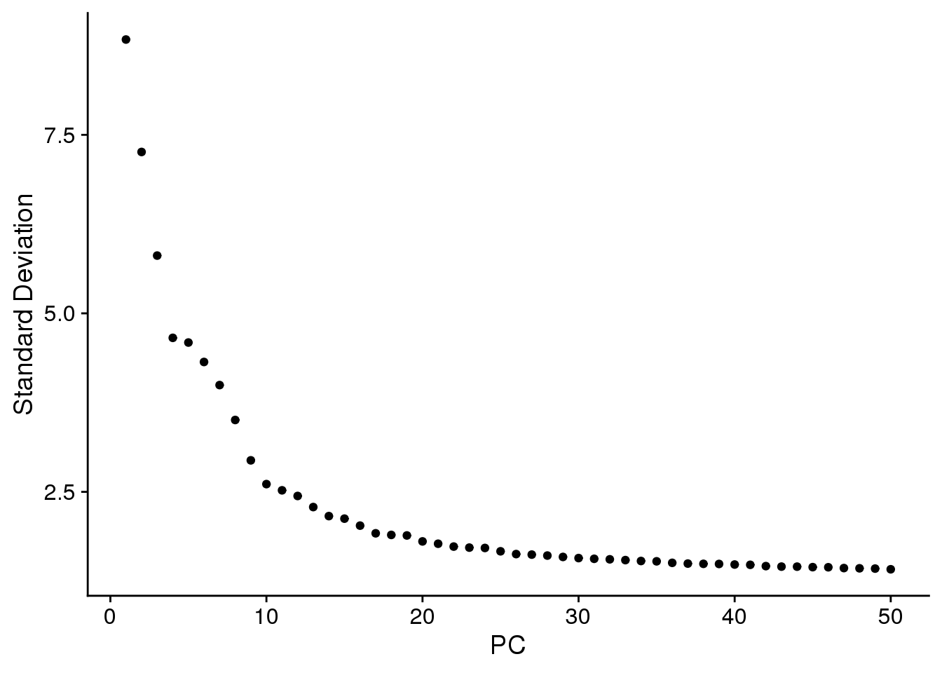

Past versions of pca-1.png

Version	Author	Date
67c1d63	Belinda Phipson	2019-10-18

VizDimLoadings(cardio.integrated, dims = 1:4, reduction = "pca")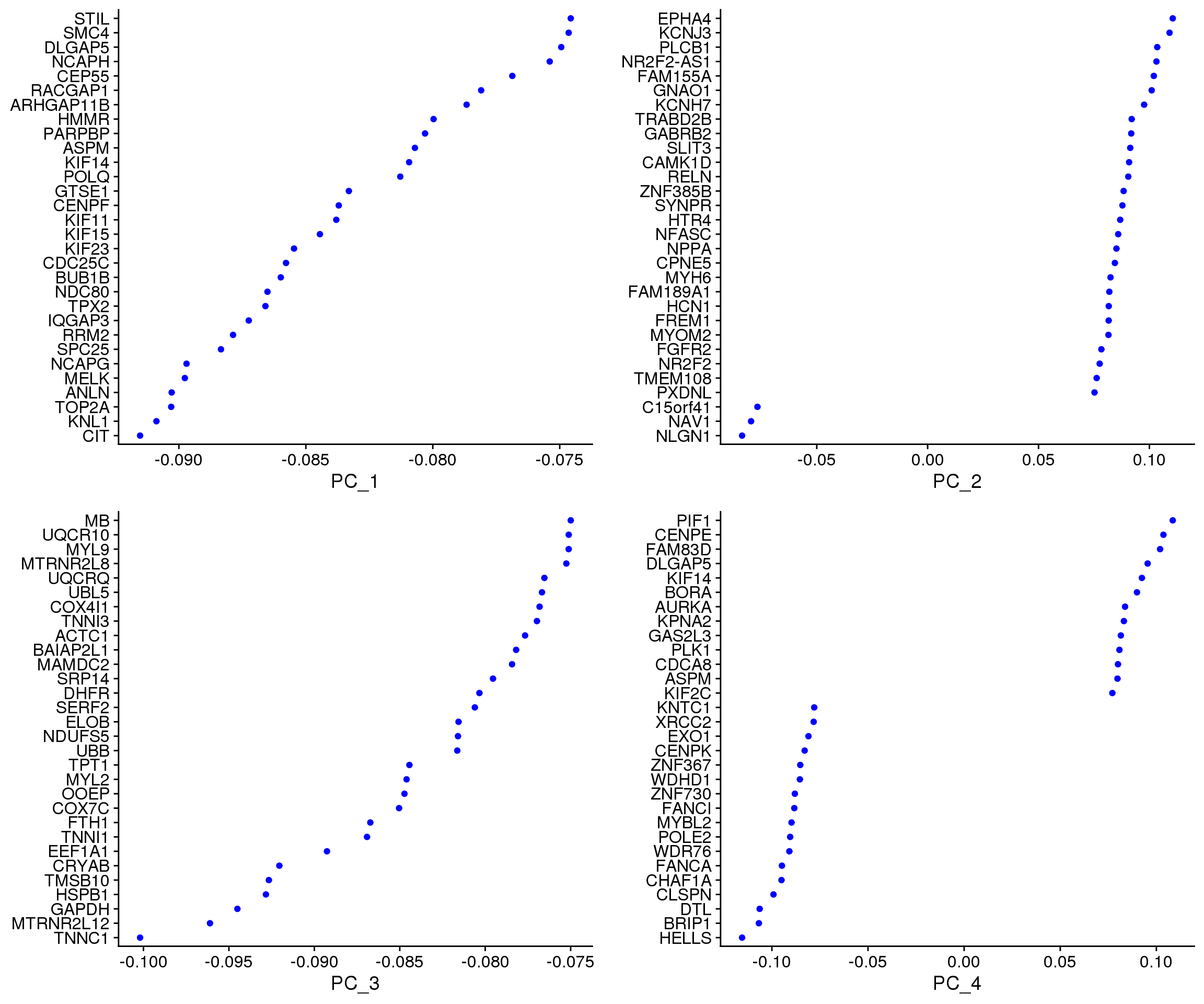

Past versions of unnamed-chunk-10-1.png

Version	Author	Date
67c1d63	Belinda Phipson	2019-10-18

DimPlot(cardio.integrated, reduction = "pca",group.by="orig.ident")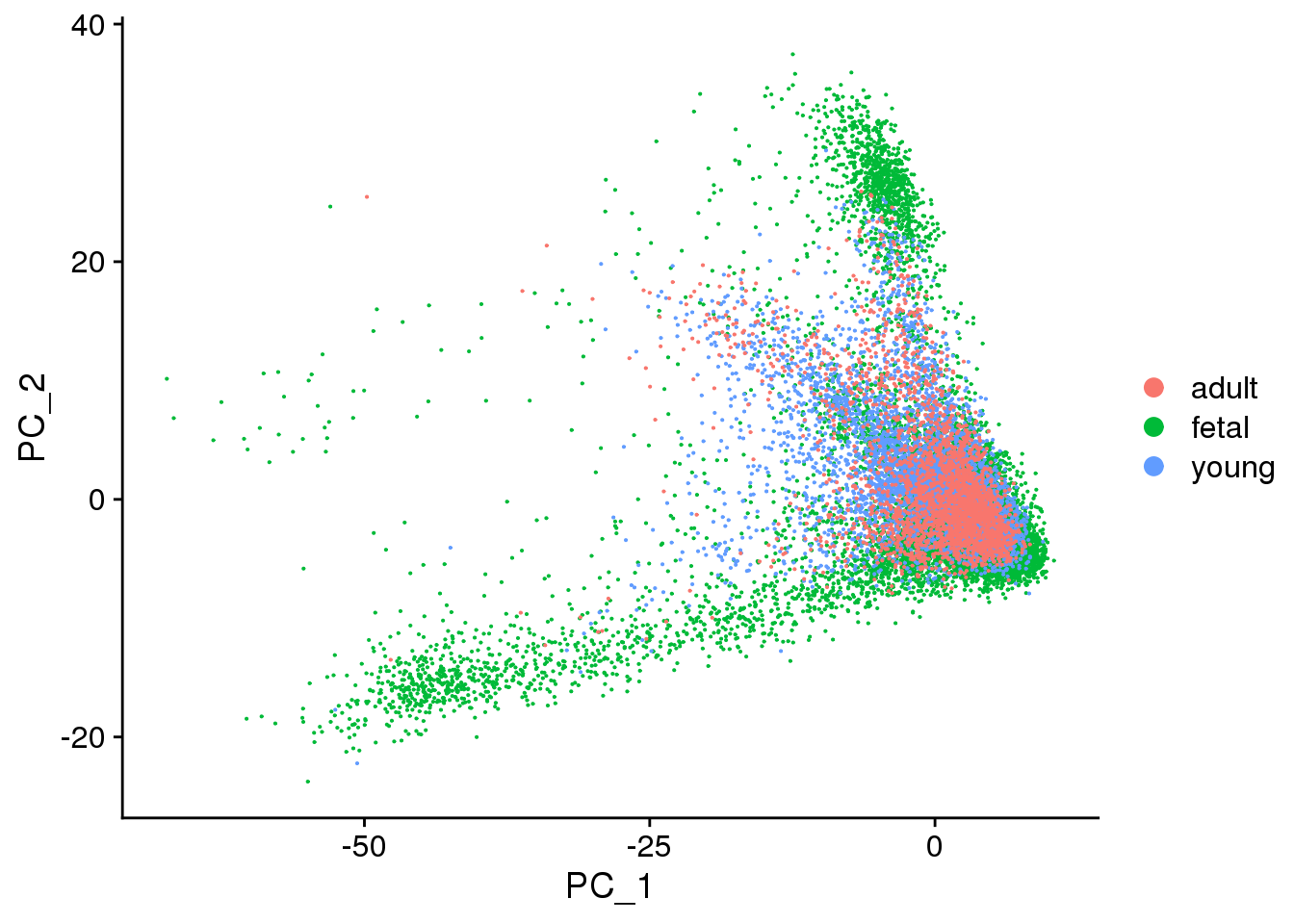

Past versions of unnamed-chunk-11-1.png

Version	Author	Date
67c1d63	Belinda Phipson	2019-10-18

DimPlot(cardio.integrated, reduction = "pca",group.by="biorep")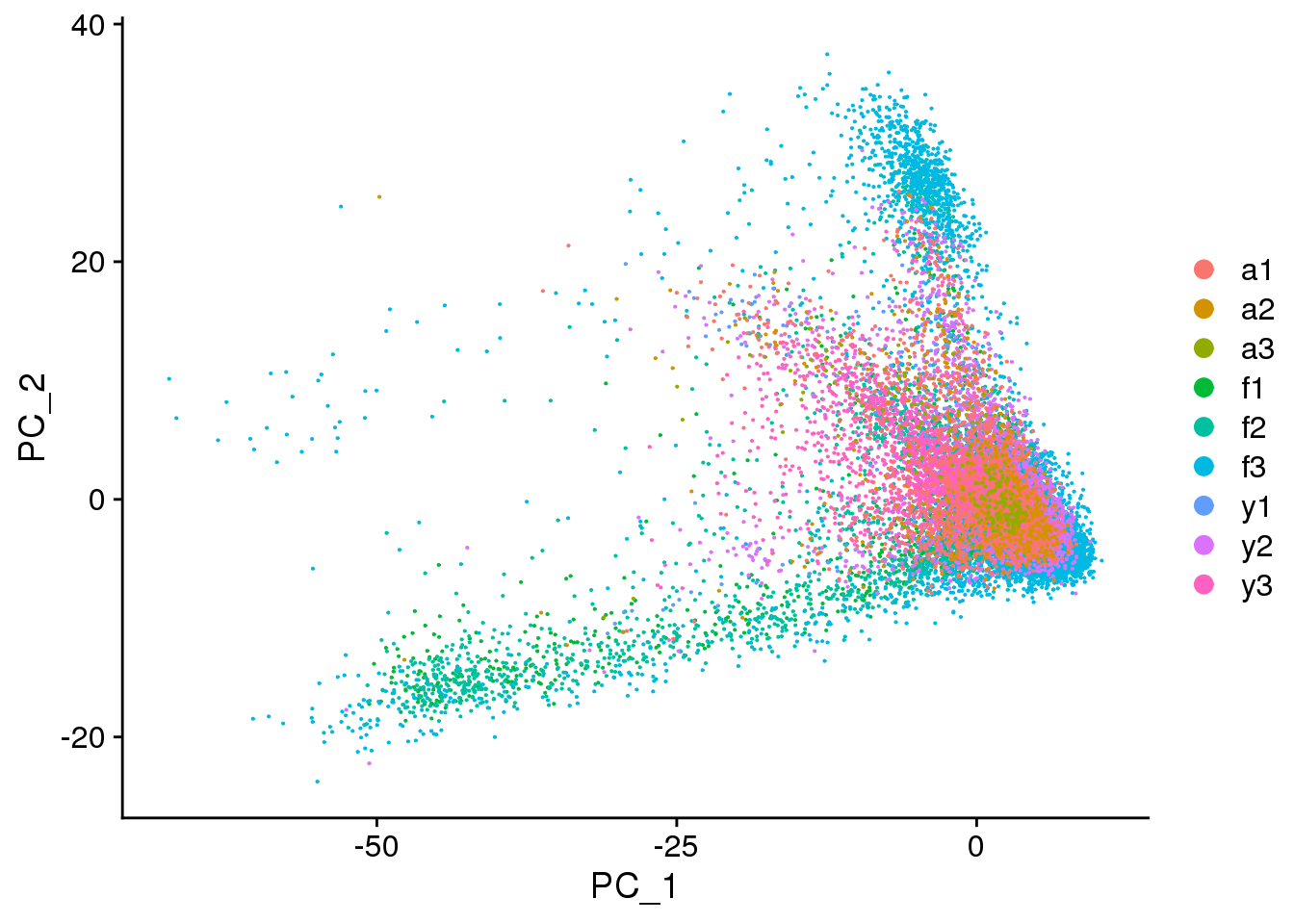

Past versions of unnamed-chunk-11-2.png

Version	Author	Date
67c1d63	Belinda Phipson	2019-10-18

DimPlot(cardio.integrated, reduction = "pca",group.by="sex")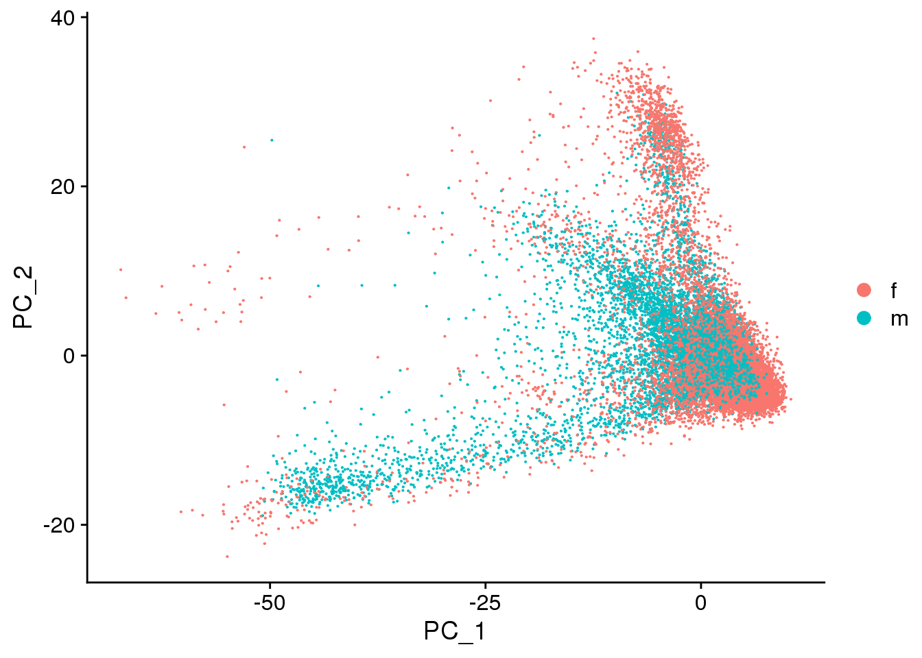

Past versions of unnamed-chunk-11-3.png

Version	Author	Date
67c1d63	Belinda Phipson	2019-10-18

DimPlot(cardio.integrated, reduction = "pca",group.by="batch")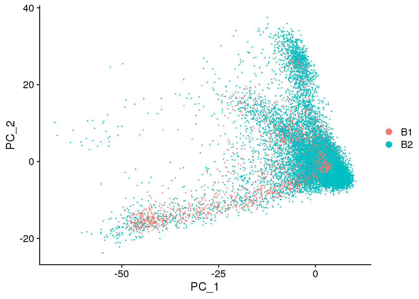

DimHeatmap(cardio.integrated, dims = 1:15, cells = 500, balanced = TRUE)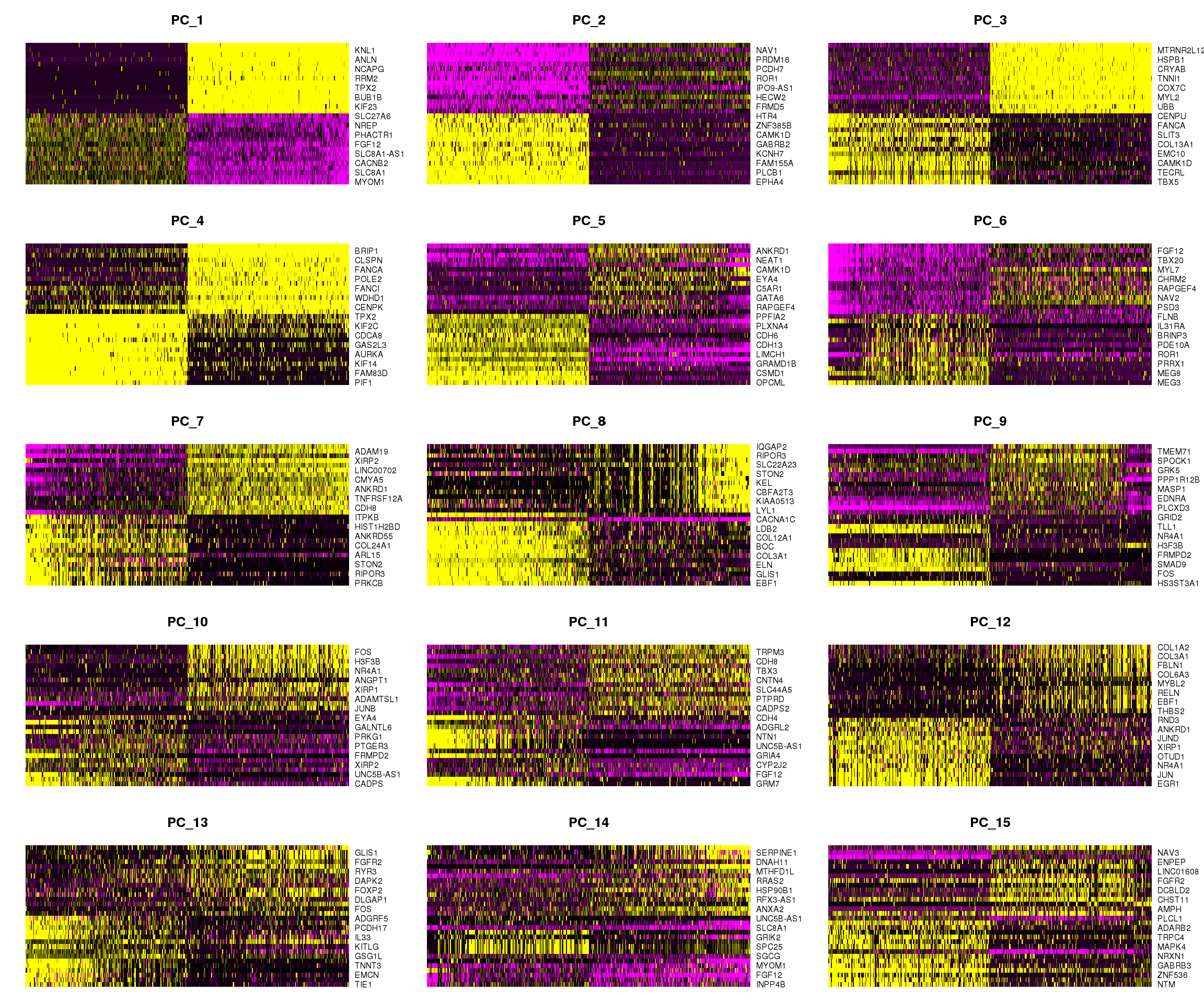

Past versions of unnamed-chunk-12-1.png

Version	Author	Date
67c1d63	Belinda Phipson	2019-10-18

DimHeatmap(cardio.integrated, dims = 16:30, cells = 500, balanced = TRUE)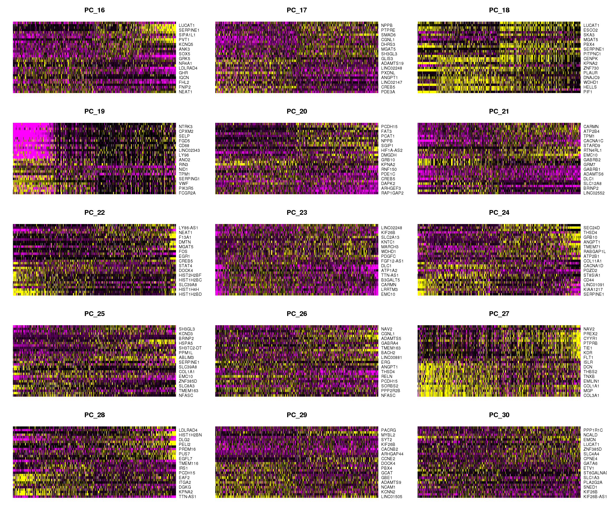

DimHeatmap(cardio.integrated, dims = 31:45, cells = 500, balanced = TRUE)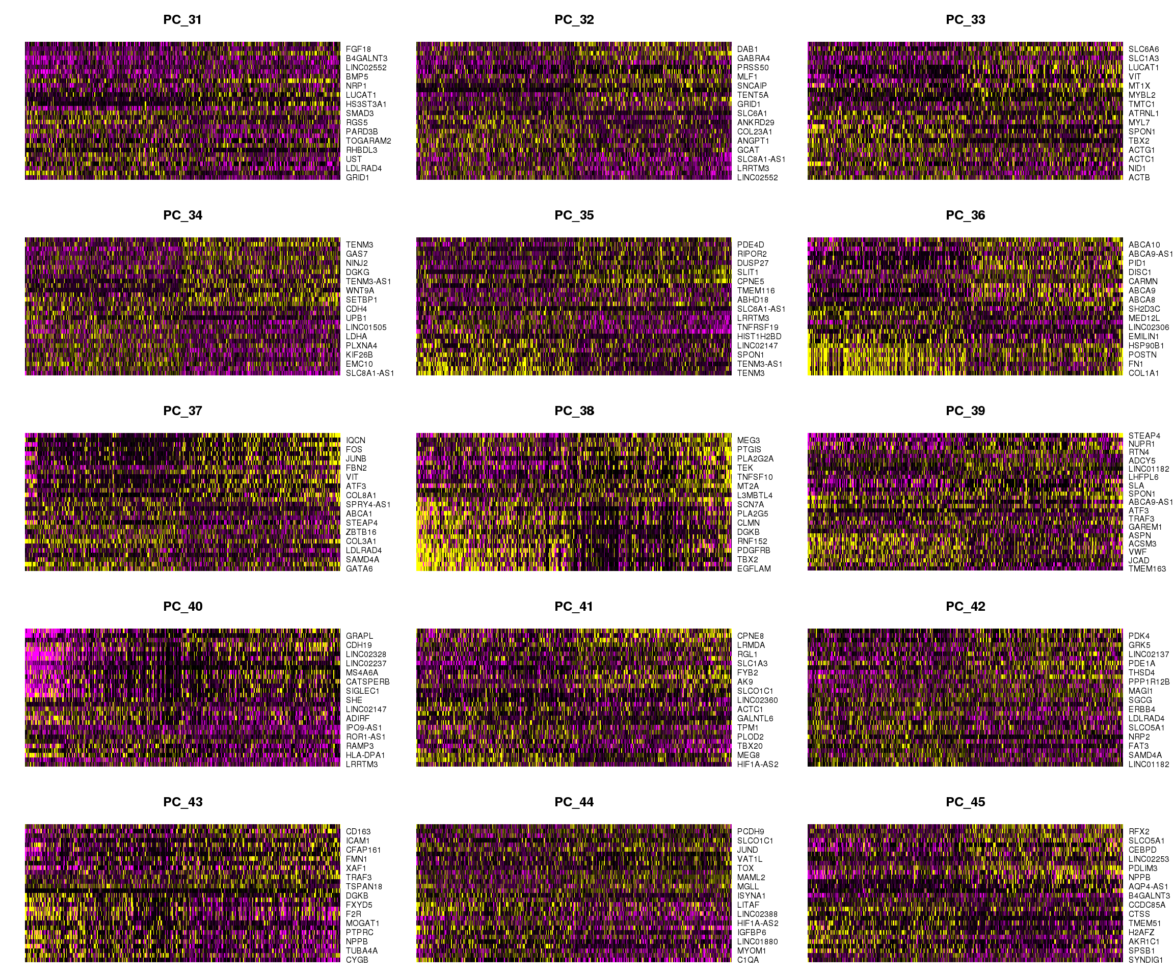

Perform nearest neighbours clustering

cardio.integrated <- FindNeighbors(cardio.integrated, dims = 1:20)
cardio.integrated <- FindClusters(cardio.integrated, resolution = 0.1)

Modularity Optimizer version 1.3.0 by Ludo Waltman and Nees Jan van Eck

Number of nodes: 27037
Number of edges: 943610

Running Louvain algorithm...
Maximum modularity in 10 random starts: 0.9410
Number of communities: 7
Elapsed time: 10 seconds

table(Idents(cardio.integrated))

    0     1     2     3     4     5     6 
18330  2849  2101  1280  1121  1016   340 

par(mar=c(5,4,2,2))
barplot(table(Idents(cardio.integrated)),ylab="Number of cells",xlab="Clusters")
title("Number of cells in each cluster")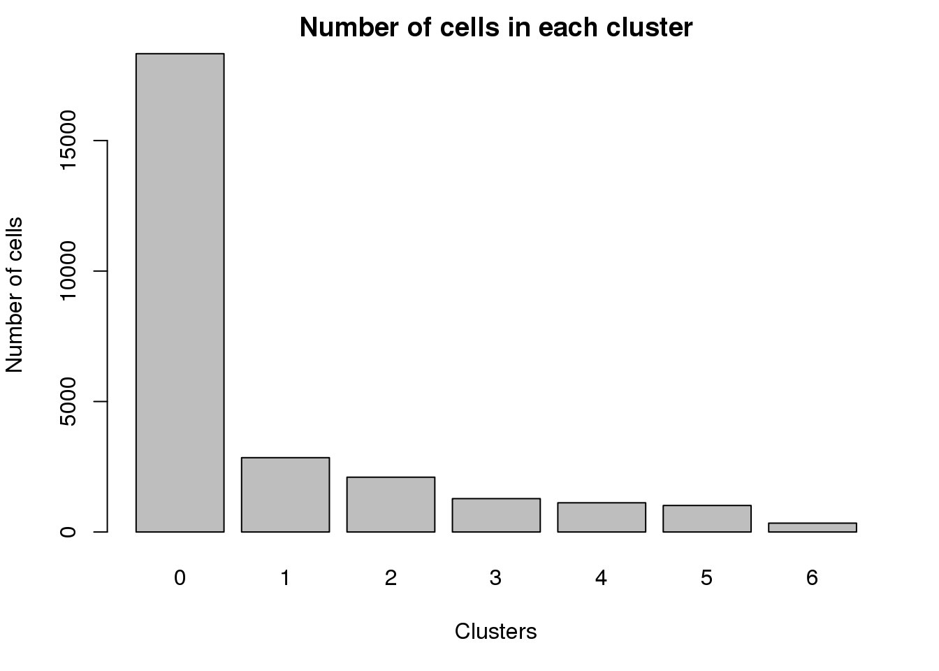

Past versions of unnamed-chunk-13-1.png

Version	Author	Date
67c1d63	Belinda Phipson	2019-10-18

Visualisation with TSNE

set.seed(10)
cardio.integrated <- RunTSNE(cardio.integrated, reduction = "pca", dims = 1:20)

DimPlot(cardio.integrated, reduction = "tsne",label=TRUE,label.size = 6,pt.size = 0.5)+NoLegend()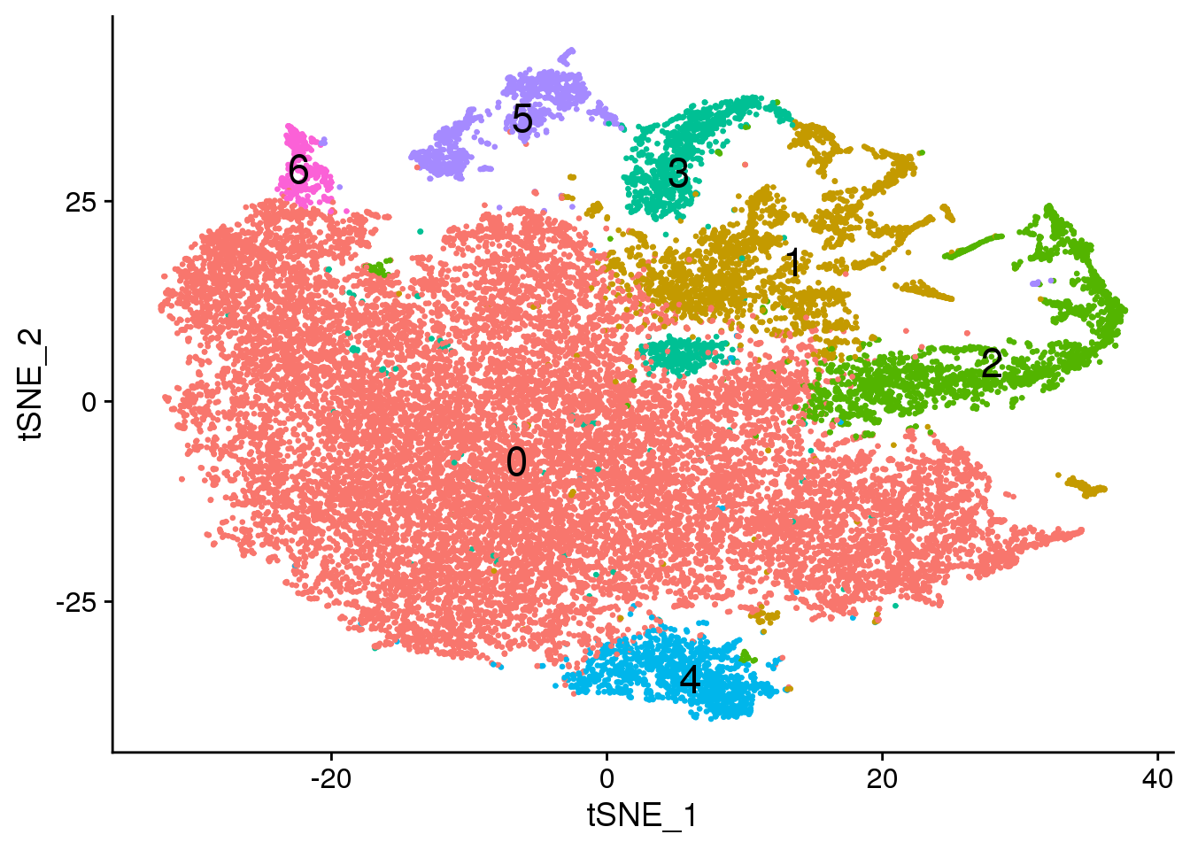

pdf(file="./output/Figures/NormalDev/tsne-cardioALL-res01.pdf",width=10,height=8,onefile = FALSE)
DimPlot(cardio.integrated, reduction = "tsne",label=TRUE,label.size = 6,pt.size = 0.5)+NoLegend()
dev.off()

png 
  2 

DimPlot(cardio.integrated, reduction = "tsne", group.by = "orig.ident")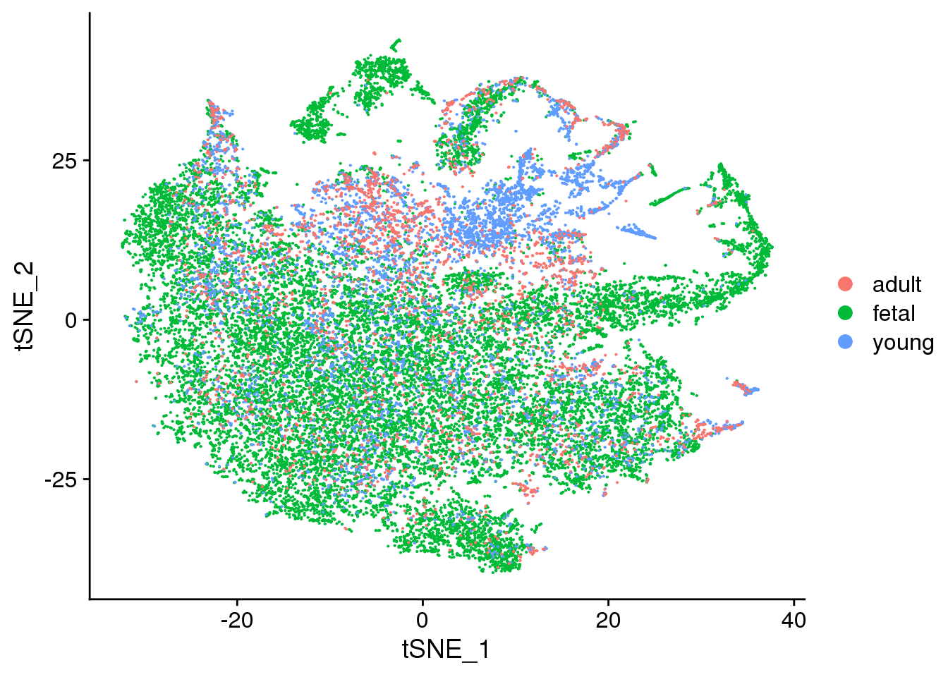

Past versions of unnamed-chunk-16-1.png

Version	Author	Date
67c1d63	Belinda Phipson	2019-10-18

DimPlot(cardio.integrated, reduction = "tsne", split.by = "orig.ident")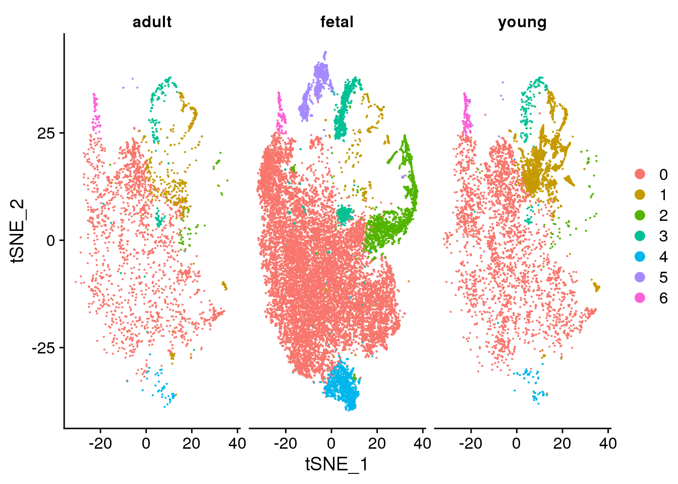

Past versions of unnamed-chunk-17-1.png

Version	Author	Date
67c1d63	Belinda Phipson	2019-10-18

DimPlot(cardio.integrated, reduction = "tsne", group.by = "biorep")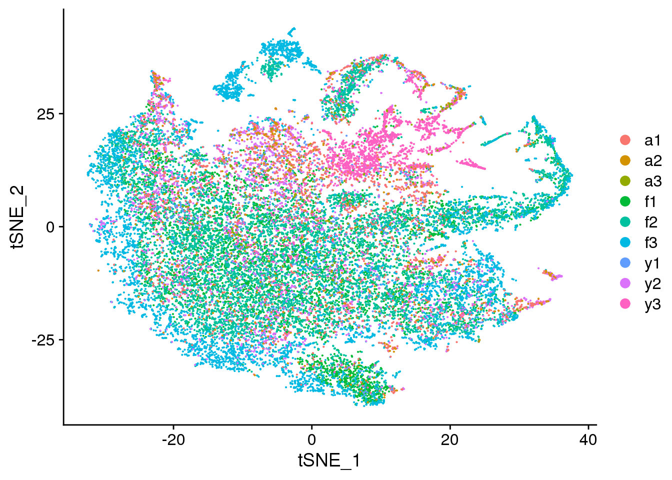

Past versions of unnamed-chunk-18-1.png

Version	Author	Date
67c1d63	Belinda Phipson	2019-10-18

DimPlot(cardio.integrated, reduction = "tsne", group.by = "sex")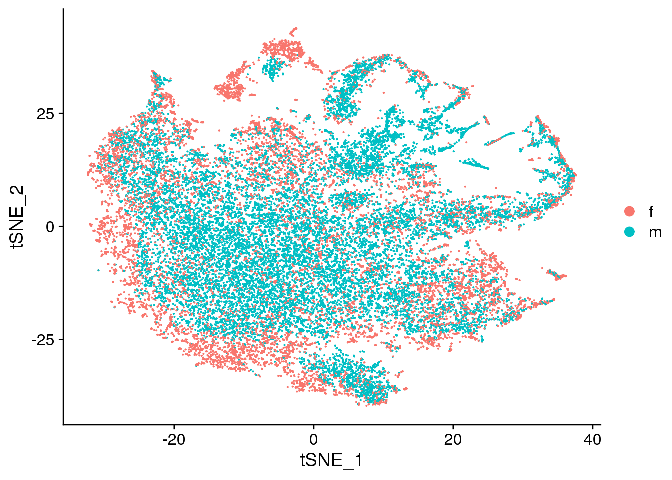

Past versions of unnamed-chunk-19-1.png

Version	Author	Date
67c1d63	Belinda Phipson	2019-10-18

DimPlot(cardio.integrated, reduction = "tsne", split.by = "sex")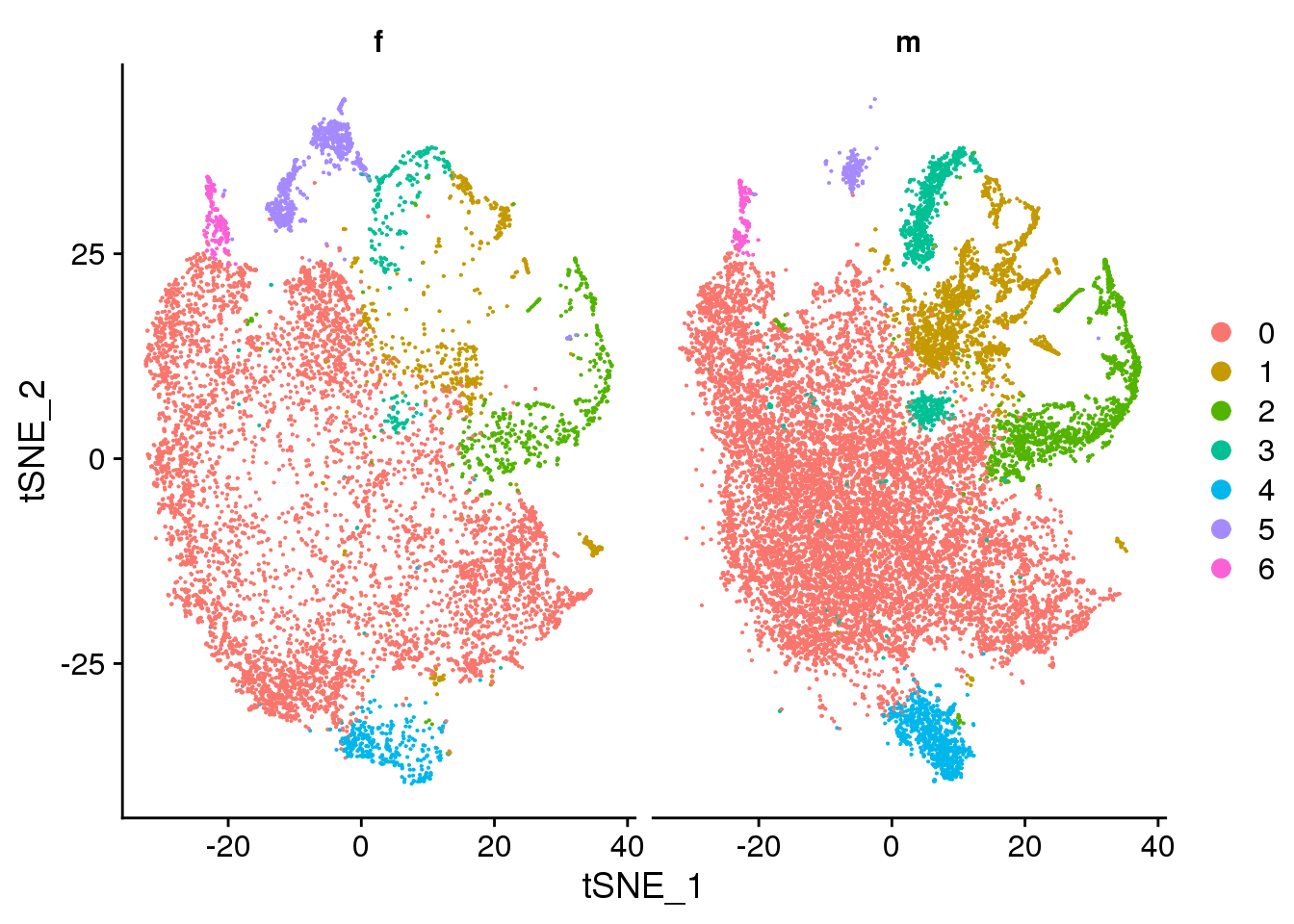

Past versions of unnamed-chunk-20-1.png

Version	Author	Date
67c1d63	Belinda Phipson	2019-10-18

DimPlot(cardio.integrated, reduction = "tsne", group.by = "batch")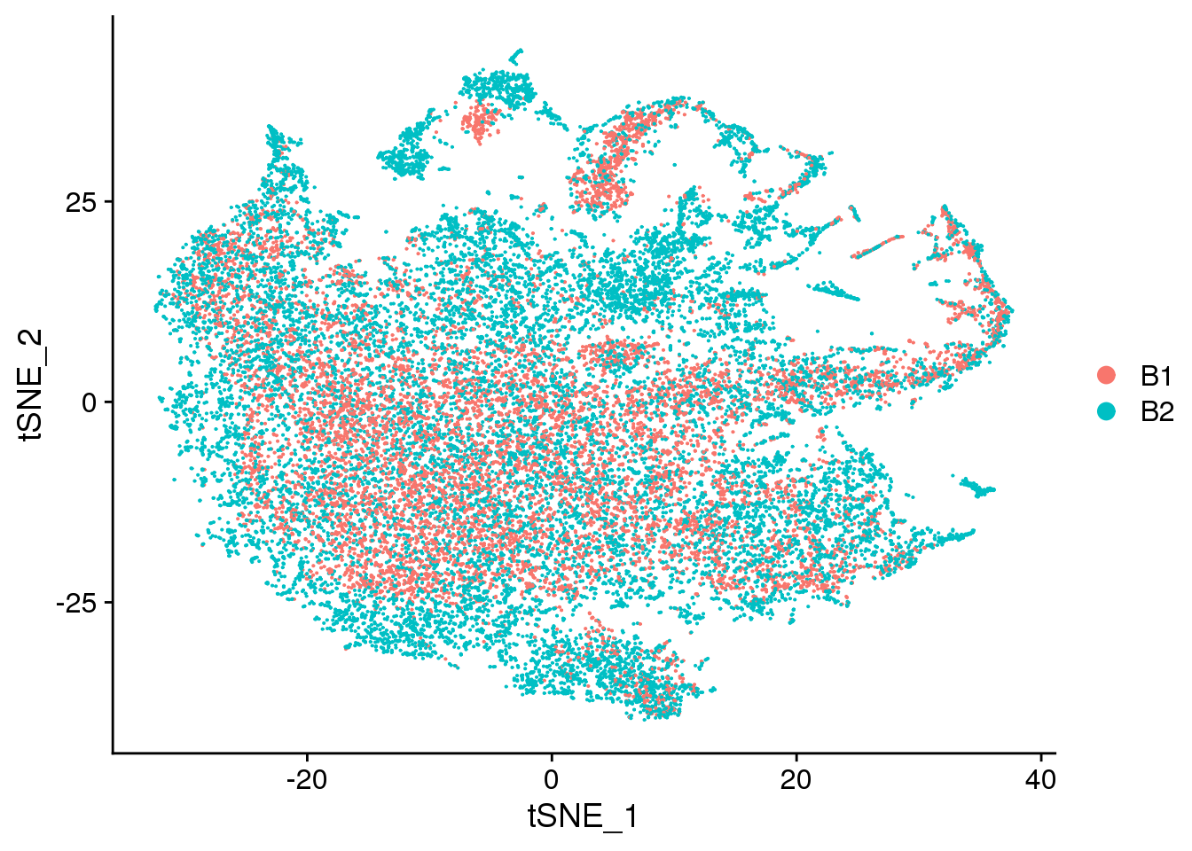

Past versions of unnamed-chunk-21-1.png

Version	Author	Date
67c1d63	Belinda Phipson	2019-10-18

par(mfrow=c(1,1))
par(mar=c(4,4,2,2))
tab <- table(Idents(cardio.integrated),cardio.integrated$biorep)
barplot(t(tab/rowSums(tab)),beside=TRUE,col=ggplotColors(9),legend=TRUE)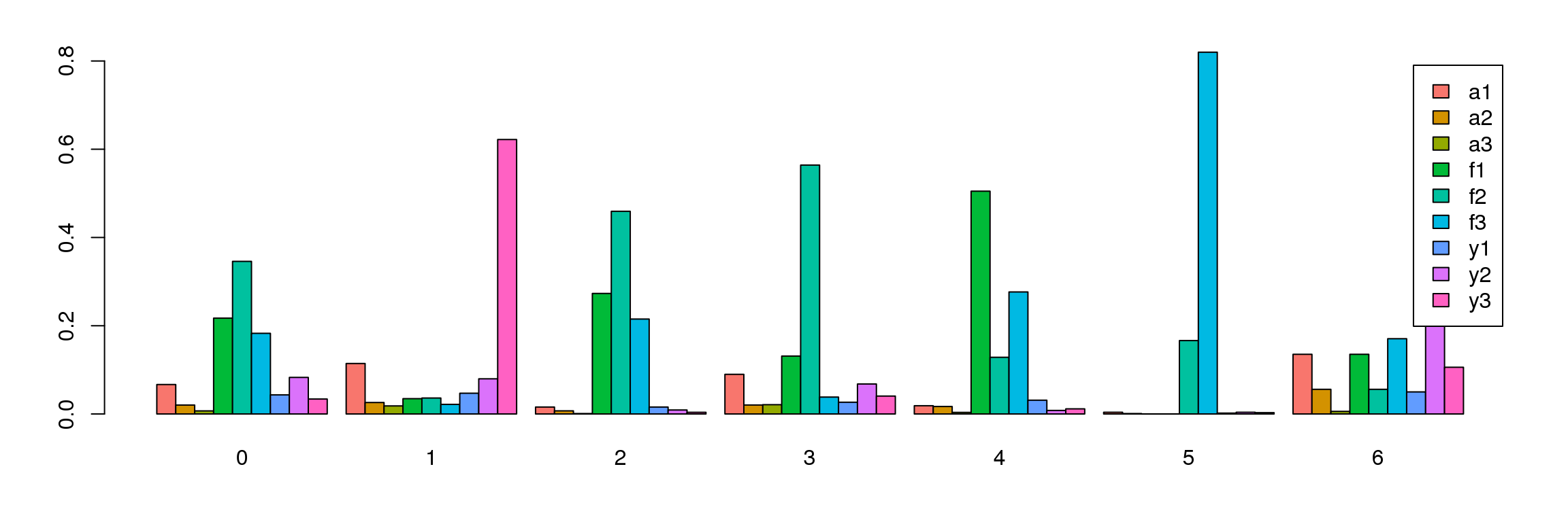

Past versions of unnamed-chunk-22-1.png

Version	Author	Date
67c1d63	Belinda Phipson	2019-10-18

par(mfrow=c(1,1))
par(mar=c(4,4,2,2))
tab <- table(Idents(cardio.integrated),cardio.integrated$orig.ident)
barplot(t(tab/rowSums(tab)),beside=TRUE,col=ggplotColors(3))
legend("topleft",legend=colnames(tab),fill=ggplotColors(3))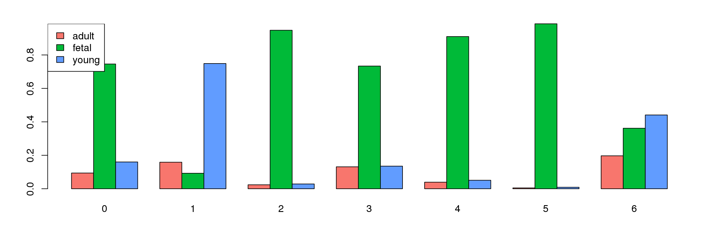

Visualisation with clustree

clusres <- c(0.1,0.2,0.3,0.4,0.5,0.6,0.7,0.8,0.9,1,1.1,1.2)

for(i in 1:length(clusres)){
  cardio.integrated <- FindClusters(cardio.integrated, 
                                   resolution = clusres[i])
}

Modularity Optimizer version 1.3.0 by Ludo Waltman and Nees Jan van Eck

Number of nodes: 27037
Number of edges: 943610

Running Louvain algorithm...
Maximum modularity in 10 random starts: 0.9410
Number of communities: 7
Elapsed time: 10 seconds
Modularity Optimizer version 1.3.0 by Ludo Waltman and Nees Jan van Eck

Number of nodes: 27037
Number of edges: 943610

Running Louvain algorithm...
Maximum modularity in 10 random starts: 0.9183
Number of communities: 11
Elapsed time: 9 seconds
Modularity Optimizer version 1.3.0 by Ludo Waltman and Nees Jan van Eck

Number of nodes: 27037
Number of edges: 943610

Running Louvain algorithm...
Maximum modularity in 10 random starts: 0.9023
Number of communities: 13
Elapsed time: 8 seconds
Modularity Optimizer version 1.3.0 by Ludo Waltman and Nees Jan van Eck

Number of nodes: 27037
Number of edges: 943610

Running Louvain algorithm...
Maximum modularity in 10 random starts: 0.8873
Number of communities: 16
Elapsed time: 10 seconds
Modularity Optimizer version 1.3.0 by Ludo Waltman and Nees Jan van Eck

Number of nodes: 27037
Number of edges: 943610

Running Louvain algorithm...
Maximum modularity in 10 random starts: 0.8735
Number of communities: 17
Elapsed time: 8 seconds
Modularity Optimizer version 1.3.0 by Ludo Waltman and Nees Jan van Eck

Number of nodes: 27037
Number of edges: 943610

Running Louvain algorithm...
Maximum modularity in 10 random starts: 0.8601
Number of communities: 18
Elapsed time: 9 seconds
Modularity Optimizer version 1.3.0 by Ludo Waltman and Nees Jan van Eck

Number of nodes: 27037
Number of edges: 943610

Running Louvain algorithm...
Maximum modularity in 10 random starts: 0.8486
Number of communities: 19
Elapsed time: 8 seconds
Modularity Optimizer version 1.3.0 by Ludo Waltman and Nees Jan van Eck

Number of nodes: 27037
Number of edges: 943610

Running Louvain algorithm...
Maximum modularity in 10 random starts: 0.8401
Number of communities: 18
Elapsed time: 9 seconds
Modularity Optimizer version 1.3.0 by Ludo Waltman and Nees Jan van Eck

Number of nodes: 27037
Number of edges: 943610

Running Louvain algorithm...
Maximum modularity in 10 random starts: 0.8299
Number of communities: 20
Elapsed time: 8 seconds
Modularity Optimizer version 1.3.0 by Ludo Waltman and Nees Jan van Eck

Number of nodes: 27037
Number of edges: 943610

Running Louvain algorithm...
Maximum modularity in 10 random starts: 0.8232
Number of communities: 23
Elapsed time: 9 seconds
Modularity Optimizer version 1.3.0 by Ludo Waltman and Nees Jan van Eck

Number of nodes: 27037
Number of edges: 943610

Running Louvain algorithm...
Maximum modularity in 10 random starts: 0.8173
Number of communities: 23
Elapsed time: 9 seconds
Modularity Optimizer version 1.3.0 by Ludo Waltman and Nees Jan van Eck

Number of nodes: 27037
Number of edges: 943610

Running Louvain algorithm...
Maximum modularity in 10 random starts: 0.8105
Number of communities: 23
Elapsed time: 7 seconds

pct.male <- function(x) {mean(x=="m")}
pct.female <- function(x) {mean(x=="f")}
pct.fetal <- function(x) {mean(x=="fetal")}
pct.young <- function(x) {mean(x=="young")}
pct.adult <- function(x) {mean(x=="adult")}

clustree(cardio.integrated, prefix = "integrated_snn_res.")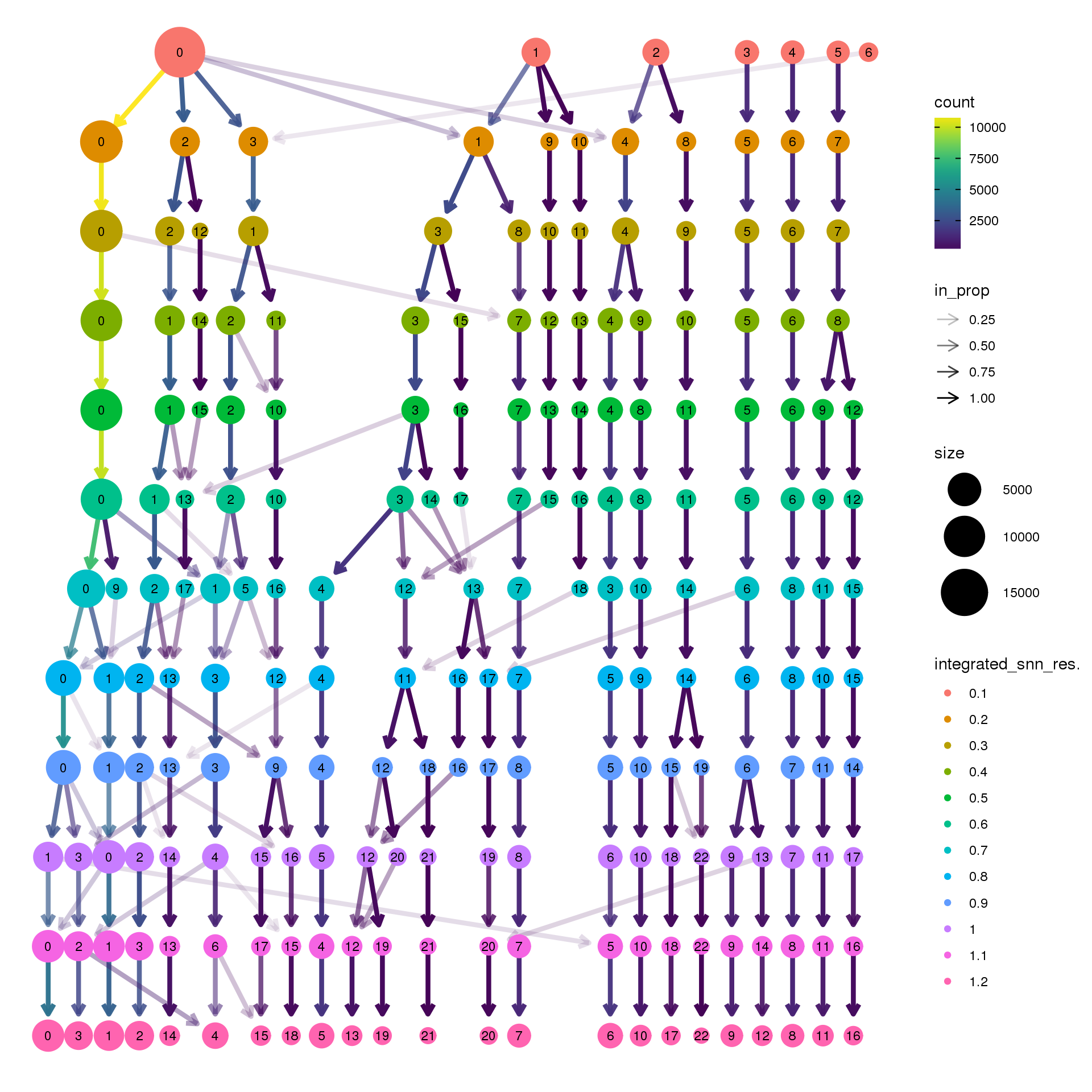

Past versions of unnamed-chunk-26-1.png

Version	Author	Date
67c1d63	Belinda Phipson	2019-10-18

clustree(cardio.integrated, prefix = "integrated_snn_res.",
         node_colour = "sex", node_colour_aggr = "pct.female",assay="RNA")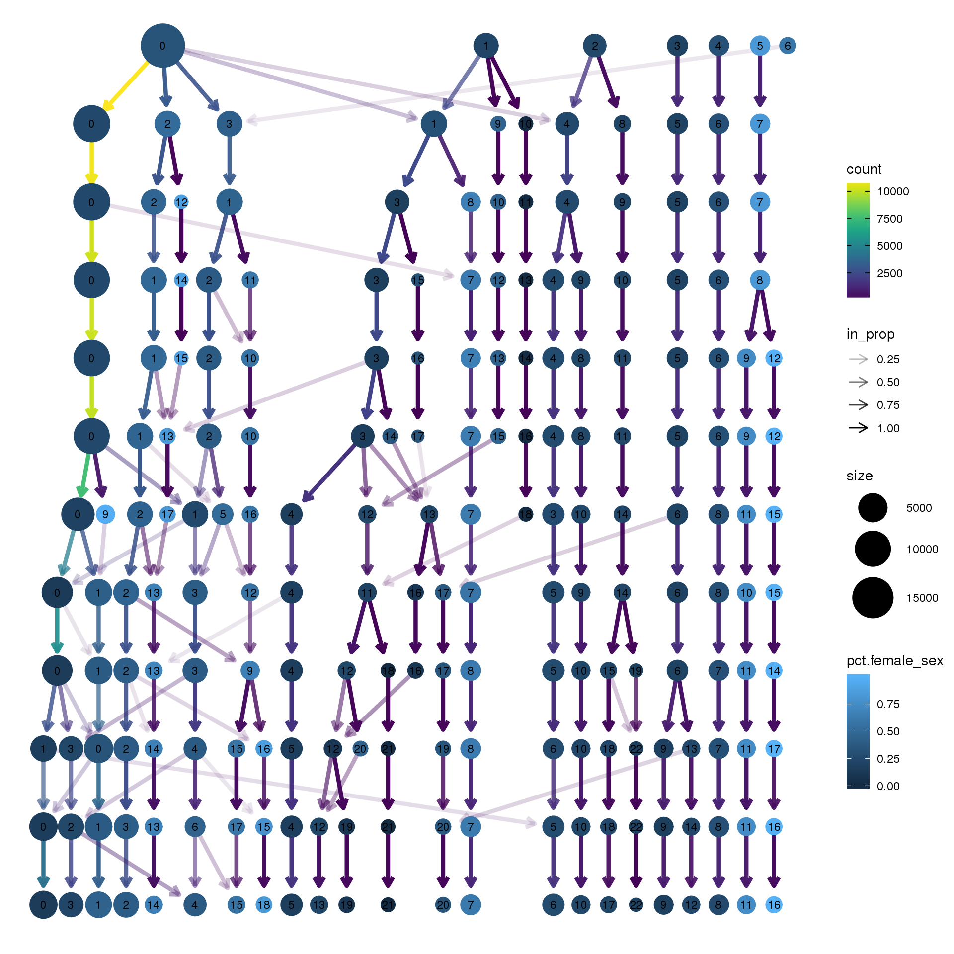

Past versions of unnamed-chunk-27-1.png

Version	Author	Date
67c1d63	Belinda Phipson	2019-10-18

clustree(cardio.integrated, prefix = "integrated_snn_res.",
         node_colour = "sex", node_colour_aggr = "pct.male",assay="RNA")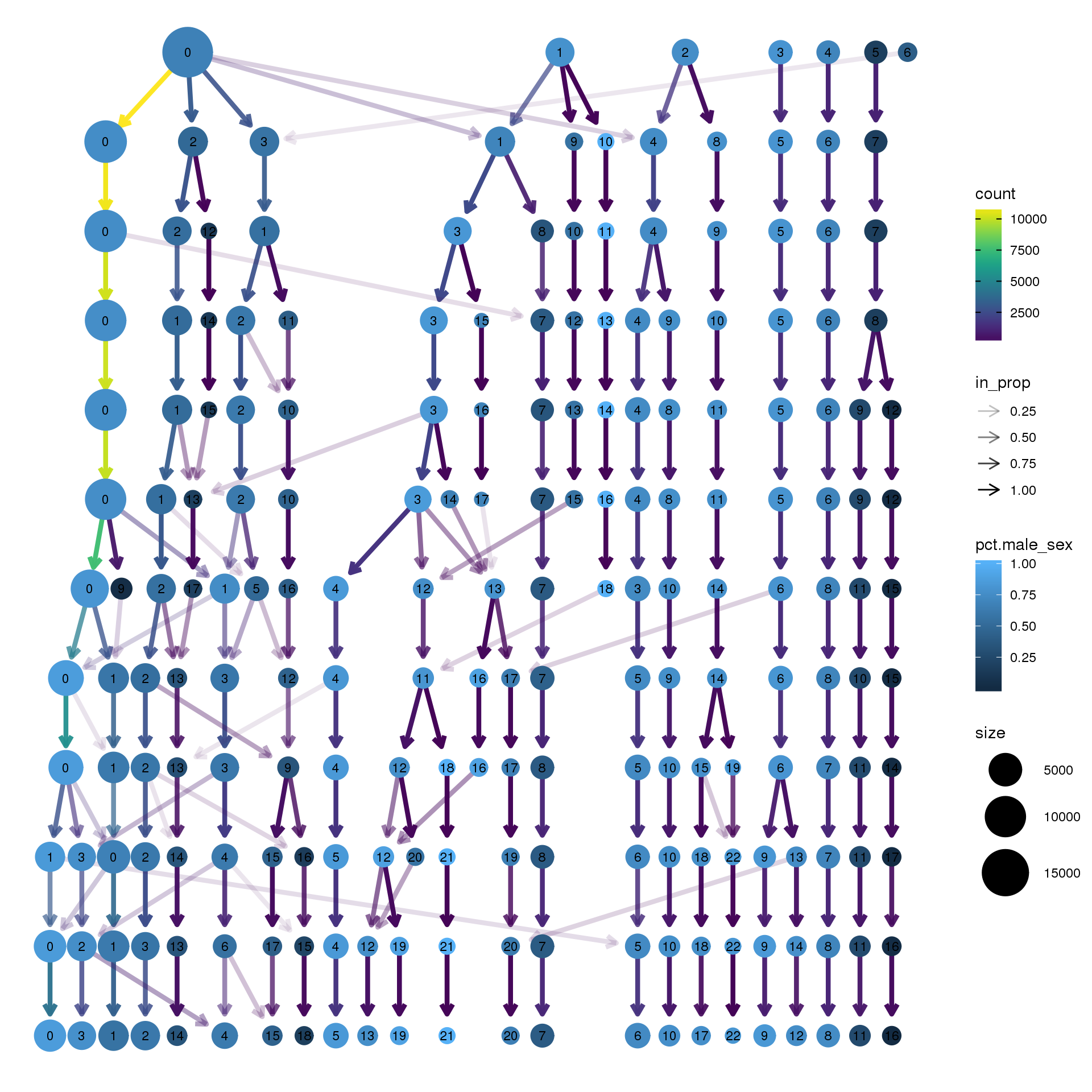

Past versions of unnamed-chunk-28-1.png

Version	Author	Date
67c1d63	Belinda Phipson	2019-10-18

clustree(cardio.integrated, prefix = "integrated_snn_res.",
         node_colour = "orig.ident", node_colour_aggr = "pct.fetal",assay="RNA")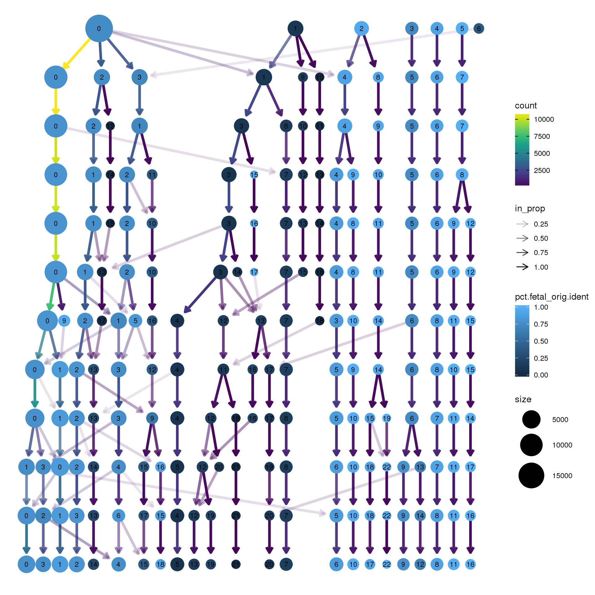

Past versions of unnamed-chunk-29-1.png

Version	Author	Date
67c1d63	Belinda Phipson	2019-10-18

clustree(cardio.integrated, prefix = "integrated_snn_res.",
         node_colour = "orig.ident", node_colour_aggr = "pct.young",assay="RNA")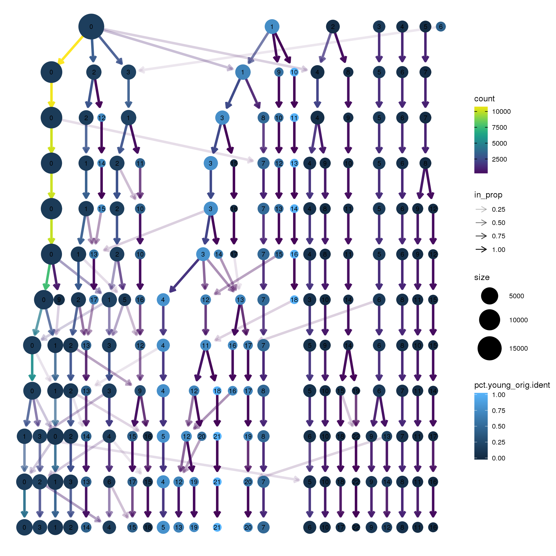

Past versions of unnamed-chunk-30-1.png

Version	Author	Date
67c1d63	Belinda Phipson	2019-10-18

clustree(cardio.integrated, prefix = "integrated_snn_res.",
         node_colour = "orig.ident", node_colour_aggr = "pct.adult",assay="RNA")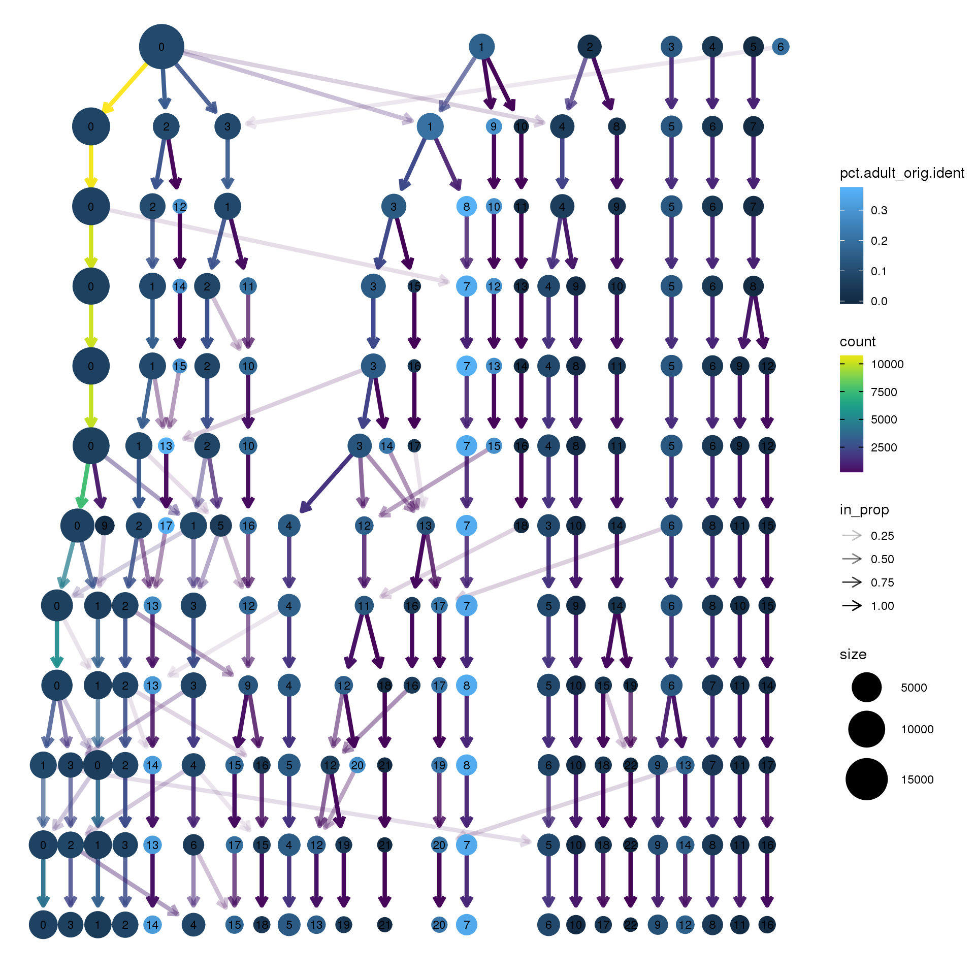

Save Seurat object

DefaultAssay(cardio.integrated) <- "RNA"
Idents(cardio.integrated) <- cardio.integrated$integrated_snn_res.0.1

saveRDS(cardio.integrated,file="./output/RDataObjects/cardio-int-FYA-filtered.Rds")
#cardio.integrated <- readRDS(file="./output/RDataObjects/cardio-int-FYA.Rds")
# Load unfiltered counts matrix for every sample (object all)
load("./output/RDataObjects/all-counts.Rdata")

columns(org.Hs.eg.db)

 [1] "ACCNUM"       "ALIAS"        "ENSEMBL"      "ENSEMBLPROT" 
 [5] "ENSEMBLTRANS" "ENTREZID"     "ENZYME"       "EVIDENCE"    
 [9] "EVIDENCEALL"  "GENENAME"     "GO"           "GOALL"       
[13] "IPI"          "MAP"          "OMIM"         "ONTOLOGY"    
[17] "ONTOLOGYALL"  "PATH"         "PFAM"         "PMID"        
[21] "PROSITE"      "REFSEQ"       "SYMBOL"       "UCSCKG"      
[25] "UNIGENE"      "UNIPROT"     

ann <- AnnotationDbi:::select(org.Hs.eg.db,keys=rownames(all),columns=c("SYMBOL","ENTREZID","ENSEMBL","GENENAME","CHR"),keytype = "SYMBOL")
m <- match(rownames(all),ann$SYMBOL)
ann <- ann[m,]
table(ann$SYMBOL==rownames(all))

 TRUE 
33939 

mito <- grep("mitochondrial",ann$GENENAME)
length(mito)

[1] 226

ribo <- grep("ribosomal",ann$GENENAME)
length(ribo)

[1] 198

missingEZID <- which(is.na(ann$ENTREZID))
length(missingEZID)

[1] 10530

Find Markers

#adultmarkers <- FindAllMarkers(adult.integrated, only.pos = TRUE, min.pct = 0.25, logfc.threshold = 0.25)
# Limma-trend for DE
m <- match(colnames(cardio.integrated),colnames(all))
all.counts <- all[,m]

chuck <- unique(c(mito,ribo,missingEZID))
length(chuck)

[1] 10875

all.counts.keep <- all.counts[-chuck,]
ann.keep <- ann[-chuck,]
table(ann.keep$SYMBOL==rownames(all.counts.keep))

 TRUE 
23064 

numzero.genes <- rowSums(all.counts.keep==0)

#avg.exp <- rowMeans(cpm.DGEList(y.kid,log=TRUE))

#plot(avg.exp,numzero.genes,xlab="Average log-normalised-counts",ylab="Number zeroes per gene")

table(numzero.genes > (ncol(all.counts.keep)-20))

FALSE  TRUE 
18407  4657 

keep.genes <- numzero.genes < (ncol(all.counts.keep)-20)
table(keep.genes)

keep.genes
FALSE  TRUE 
 4698 18366 

all.keep <- all.counts.keep[keep.genes,]
dim(all.keep)

[1] 18366 27037

ann.keep <- ann.keep[keep.genes,]

y.cardio <- DGEList(all.keep)

logcounts <- normCounts(y.cardio,log=TRUE,prior.count=0.5)

#logcounts.n <- normalizeBetweenArrays(logcounts, method = "cyclicloess")

maxclust <- length(levels(Idents(cardio.integrated)))-1

grp <- paste("c",Idents(cardio.integrated),sep = "")
grp <- factor(grp,levels = paste("c",0:maxclust,sep=""))

design <- model.matrix(~0+grp+cardio.integrated$biorep)
colnames(design)[1:(maxclust+1)] <- levels(grp)

mycont <- matrix(0,ncol=length(levels(grp)),nrow=length(levels(grp)))
colnames(mycont)<-levels(grp)
diag(mycont)<-1
mycont[upper.tri(mycont)]<- -1/(length(levels(factor(grp)))-1)
mycont[lower.tri(mycont)]<- -1/(length(levels(factor(grp)))-1)

# Fill out remaining rows with 0s
zero.rows <- matrix(0,ncol=length(levels(grp)),nrow=(ncol(design)-length(levels(Idents(cardio.integrated)))))
test <- rbind(mycont,zero.rows)


fit <- lmFit(logcounts,design)
fit.cont <- contrasts.fit(fit,contrasts=test)
fit.cont <- eBayes(fit.cont,trend=TRUE,robust=TRUE)

fit.cont$genes <- ann.keep

summary(decideTests(fit.cont))

          c0    c1    c2    c3    c4    c5    c6
Down    7235  4032  2697  5758  6760  3880  2650
NotSig  8667  8790  9107  9337 10182 11538 14120
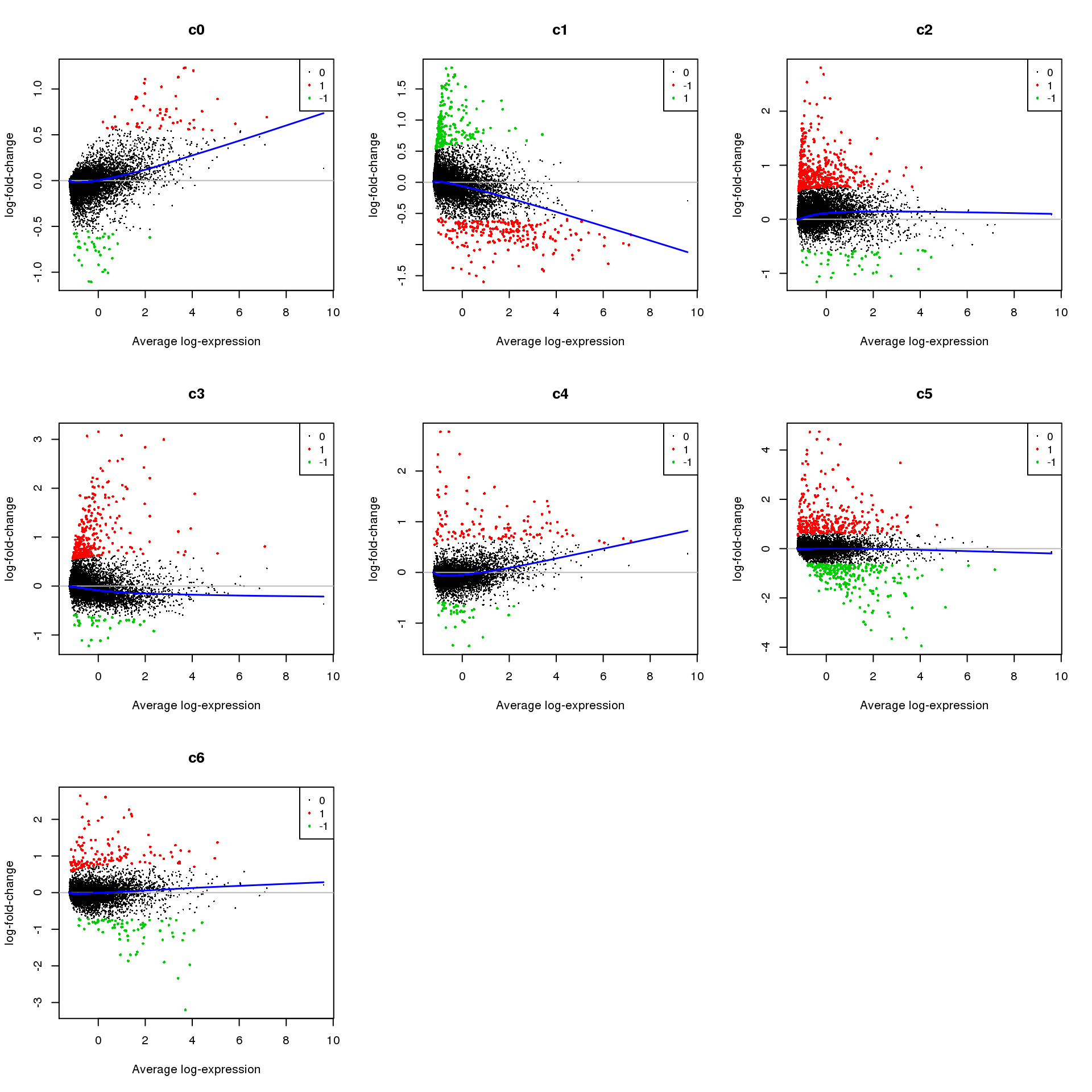
Up      2464  5544  6562  3271  1424  2948  1596

treat <- treat(fit.cont,lfc=0.5)

dt <- decideTests(treat)
summary(dt)

          c0    c1    c2    c3    c4    c5    c6
Down      39   231    48    37    42   253    71
NotSig 18274 17920 17850 18045 18208 17808 18163
Up        53   215   468   284   116   305   132

par(mfrow=c(3,3))
for(i in 1:ncol(mycont)){
  plotMD(treat,coef=i,status = dt[,i],hl.cex=0.5)
  abline(h=0,col=colours()[c(226)])
  lines(lowess(treat$Amean,treat$coefficients[,i]),lwd=1.5,col=4)
}

Write out marker genes for each cluster

contnames <- colnames(mycont)

for(i in 1:length(contnames)){
  topsig <- topTreat(treat,coef=i,n=Inf)
  write.csv(topsig,file=paste("./output/MarkerAnalysis/Cardiomyocytes/Development/Filtered/Cluster-",contnames[i],".csv",sep=""))
}

fdr <- apply(treat$p.value, 2, function(x) p.adjust(x, method="BH"))
output <- data.frame(treat$genes,LogFC=treat$coefficients,AveExp=treat$Amean,tstat=treat$t, pvalue=treat$p.value, fdr=fdr)
write.csv(output,file="./output/MarkerAnalysis/Cardiomyocytes/Development/Filtered/MarkerAnalysis.csv")

Perform gene set testing on C2 and GO sets

contnames <- colnames(mycont)

load("./output/RDataObjects/human_c2_v5p2.rdata")
load("./output/RDataObjects/human_c5_v5p2.rdata")

c2.id <- ids2indices(Hs.c2,treat$genes$ENTREZID)
c5.id <- ids2indices(Hs.c5,treat$genes$ENTREZID)

reactome.id <-c2.id[grep("REACTOME",names(c2.id))]

c2.c0 <- cameraPR(treat$t[,1],c2.id)
reactome.c0 <- cameraPR(treat$t[,1],reactome.id)
go.c0 <- cameraPR(treat$t[,1],c5.id)

for(i in 1:length(contnames)){
  write.csv(cameraPR(treat$t[,i],c2.id),file=paste("./output/MarkerAnalysis/Cardiomyocytes/Development/Filtered/c2-",contnames[i],".csv",sep=""))
  write.csv(cameraPR(treat$t[,i],reactome.id),file=paste("./output/MarkerAnalysis/Cardiomyocytes/Development/Filtered/reactome-",contnames[i],".csv",sep=""))
  write.csv(cameraPR(treat$t[,i],c5.id),file=paste("./output/MarkerAnalysis/Cardiomyocytes/Development/Filtered/go-",contnames[i],".csv",sep=""))
}

Check quality of clusters

The quality of the clusters look good.

par(mfrow=c(1,1))
numgenes <- colSums(all.keep!=0)
boxplot(numgenes~grp)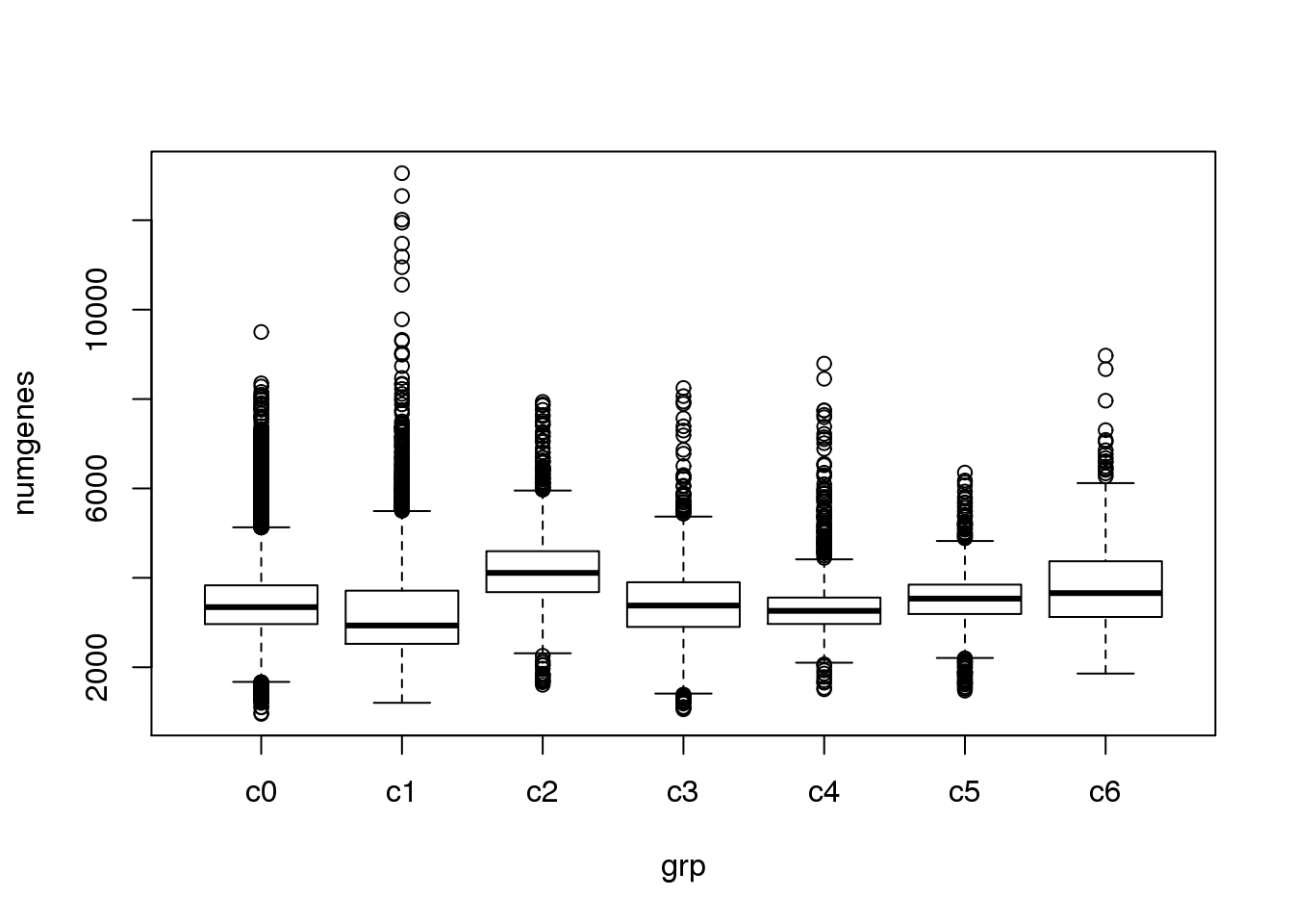

Heatmap of marker genes

sam <- factor(cardio.integrated$biorep,levels=c("f1","f2","f3","y1","y2","y3","a1","a2","a3"))
newgrp <- paste(grp,sam,sep=".")
newgrp <- factor(newgrp,levels=paste(rep(levels(grp),each=9),levels(sam),sep="."))
o <-order(newgrp)
clust <- rep(levels(grp),each=9)
samps <- rep(levels(sam),length(levels(grp)))

Summarise expression across cells

sumexpr <- matrix(NA,nrow=nrow(logcounts),ncol=length(levels(newgrp)))
rownames(sumexpr) <- rownames(logcounts)
colnames(sumexpr) <- levels(newgrp)

for(i in 1:nrow(sumexpr)){
  sumexpr[i,] <- tapply(logcounts[i,],newgrp,mean)
}

sig.genes <- gene.label <- vector("list", length(levels(grp)))
for(i in 1:length(sig.genes)){
  top <- topTreat(treat,coef=i,n=Inf)
  sig.genes[[i]] <- rownames(top)[top$logFC>0][1:10]
  gene.label[[i]] <- paste(rownames(top)[top$logFC>0][1:10],levels(grp)[i],sep="-")
} 

csig <- unlist(sig.genes)
genes <- unlist(gene.label)

myColors <- list(Clust=NA,Sample=NA)
myColors$Clust<-sample(ggplotColors(length(levels(grp))),length(levels(grp)))
names(myColors$Clust)<-levels(grp)
myColors$Sample <- sample(ggplotColors(length(levels(sam))),length(levels(sam)))
names(myColors$Sample) <- levels(sam)


pdf(file="./output/Figures/NormalDev/cardio-heatmap-siggenes-summarised-FYA-filtered.pdf",width=20,height=20,onefile = FALSE)
aheatmap(sumexpr[csig,],Rowv = NA,Colv = NA, labRow = genes,
         annCol=list(Clust=clust,Sample=samps),
         annColors=myColors,
         fontsize=16,color="-RdYlBu",
         scale="none")
dev.off()

png 
  2 

aheatmap(sumexpr[csig,],Rowv = NA,Colv = NA, labRow = genes,
         annCol=list(Clust=clust,Sample=samps),
         annColors=myColors,
         fontsize=16,color="-RdYlBu",
         scale="none")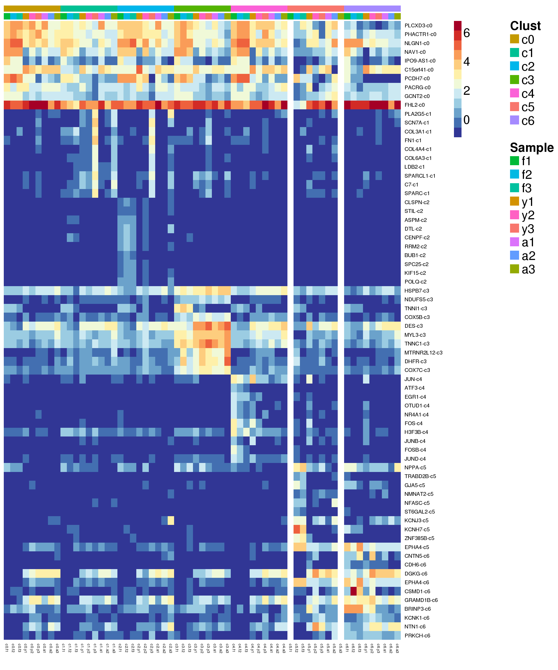

Past versions of unnamed-chunk-46-1.png

Version	Author	Date
67c1d63	Belinda Phipson	2019-10-18

Heatmap of pre-identified heart genes

hm <- read.delim("./data/heart-markers-long.txt",stringsAsFactors = FALSE)
hgene <- toupper(hm$Gene)
hgene <- unique(hgene)

m <- match(hgene,rownames(sumexpr))
m <- m[!is.na(m)]

mycelltypes <- hm$Celltype[match(rownames(sumexpr)[m],toupper(hm$Gene))]
mycelltypes <- factor(mycelltypes)

mygenes <- rownames(sumexpr)[m]
mygenelab <- paste(mygenes,mycelltypes,sep="_")

pdf(file="./output/Figures/NormalDev/cardio-heatmap-hmarkers-summarised-FYA-filtered.pdf",width=20,height=15,onefile = FALSE)
aheatmap(sumexpr[m,],Rowv = NA,Colv = NA, labRow = mygenelab,
         annCol=list(Clust=clust,Sample=samps),
 #        annRow=list(Celltypes=mycelltypes),
         annColors=myColors,
         fontsize=14,color="-RdYlBu")
dev.off()

png 
  2 

aheatmap(sumexpr[m,],Rowv = NA,Colv = NA, labRow = mygenelab,
         annCol=list(Clust=clust,Sample=samps),
 #        annRow=list(Celltypes=mycelltypes),
         annColors=myColors,
         fontsize=14,color="-RdYlBu")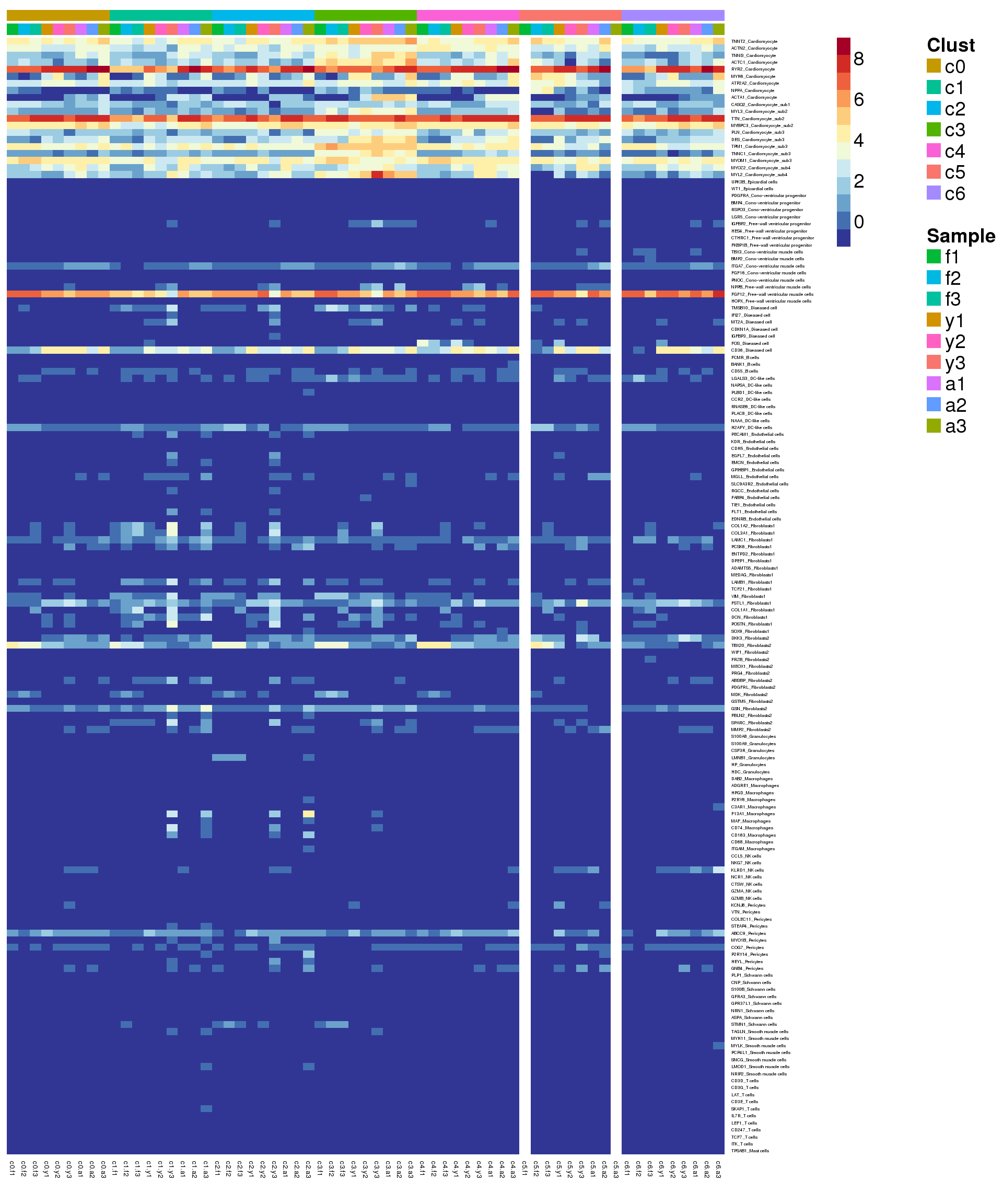

Session information

sessionInfo()

R version 3.6.0 (2019-04-26)
Platform: x86_64-pc-linux-gnu (64-bit)
Running under: CentOS release 6.7 (Final)

Matrix products: default
BLAS:   /usr/local/installed/R/3.6.0/lib64/R/lib/libRblas.so
LAPACK: /usr/local/installed/R/3.6.0/lib64/R/lib/libRlapack.so

locale:
 [1] LC_CTYPE=en_US.UTF-8       LC_NUMERIC=C              
 [3] LC_TIME=en_US.UTF-8        LC_COLLATE=en_US.UTF-8    
 [5] LC_MONETARY=en_US.UTF-8    LC_MESSAGES=en_US.UTF-8   
 [7] LC_PAPER=en_US.UTF-8       LC_NAME=C                 
 [9] LC_ADDRESS=C               LC_TELEPHONE=C            
[11] LC_MEASUREMENT=en_US.UTF-8 LC_IDENTIFICATION=C       

attached base packages:
 [1] splines   parallel  stats4    stats     graphics  grDevices utils    
 [8] datasets  methods   base     

other attached packages:
 [1] dplyr_0.8.3                 clustree_0.4.0             
 [3] ggraph_1.0.2                workflowr_1.3.0            
 [5] NMF_0.21.0                  bigmemory_4.5.33           
 [7] cluster_2.1.0               rngtools_1.4               
 [9] pkgmaker_0.27               registry_0.5-1             
[11] scran_1.12.0                SingleCellExperiment_1.6.0 
[13] SummarizedExperiment_1.14.1 GenomicRanges_1.36.0       
[15] GenomeInfoDb_1.20.0         DelayedArray_0.10.0        
[17] BiocParallel_1.18.1         matrixStats_0.55.0         
[19] cowplot_1.0.0               monocle_2.12.0             
[21] DDRTree_0.1.5               irlba_2.3.3                
[23] VGAM_1.1-1                  ggplot2_3.2.1              
[25] Matrix_1.2-17               Seurat_3.0.3.9019          
[27] org.Hs.eg.db_3.8.2          AnnotationDbi_1.46.1       
[29] IRanges_2.18.1              S4Vectors_0.22.0           
[31] Biobase_2.44.0              BiocGenerics_0.30.0        
[33] RColorBrewer_1.1-2          edgeR_3.26.3               
[35] limma_3.40.2               

loaded via a namespace (and not attached):
  [1] reticulate_1.13          R.utils_2.9.0           
  [3] tidyselect_0.2.5         RSQLite_2.1.2           
  [5] htmlwidgets_1.5          grid_3.6.0              
  [7] combinat_0.0-8           docopt_0.6.1            
  [9] Rtsne_0.15               munsell_0.5.0           
 [11] codetools_0.2-16         ica_1.0-2               
 [13] statmod_1.4.30           future_1.14.0           
 [15] withr_2.1.2              colorspace_1.4-1        
 [17] fastICA_1.2-2            knitr_1.25              
 [19] ROCR_1.0-7               gbRd_0.4-11             
 [21] listenv_0.7.0            labeling_0.3            
 [23] Rdpack_0.11-0            git2r_0.26.1            
 [25] slam_0.1-45              GenomeInfoDbData_1.2.1  
 [27] polyclip_1.10-0          farver_1.1.0            
 [29] bit64_0.9-7              pheatmap_1.0.12         
 [31] rprojroot_1.3-2          vctrs_0.2.0             
 [33] xfun_0.10                R6_2.4.0                
 [35] doParallel_1.0.15        ggbeeswarm_0.6.0        
 [37] rsvd_1.0.2               locfit_1.5-9.1          
 [39] bitops_1.0-6             assertthat_0.2.1        
 [41] SDMTools_1.1-221.1       scales_1.0.0            
 [43] beeswarm_0.2.3           gtable_0.3.0            
 [45] npsurv_0.4-0             globals_0.12.4          
 [47] tidygraph_1.1.2          rlang_0.4.0             
 [49] zeallot_0.1.0            lazyeval_0.2.2          
 [51] checkmate_1.9.4          yaml_2.2.0              
 [53] reshape2_1.4.3           backports_1.1.5         
 [55] tools_3.6.0              gridBase_0.4-7          
 [57] gplots_3.0.1.1           dynamicTreeCut_1.63-1   
 [59] ggridges_0.5.1           Rcpp_1.0.2              
 [61] plyr_1.8.4               zlibbioc_1.30.0         
 [63] purrr_0.3.2              RCurl_1.95-4.12         
 [65] densityClust_0.3         pbapply_1.4-1           
 [67] viridis_0.5.1            zoo_1.8-6               
 [69] ggrepel_0.8.1            fs_1.3.1                
 [71] magrittr_1.5             data.table_1.12.4       
 [73] lmtest_0.9-37            RANN_2.6.1              
 [75] whisker_0.3-2            fitdistrplus_1.0-14     
 [77] lsei_1.2-0               evaluate_0.14           
 [79] xtable_1.8-4             sparsesvd_0.1-4         
 [81] gridExtra_2.3            HSMMSingleCell_1.4.0    
 [83] compiler_3.6.0           scater_1.12.2           
 [85] tibble_2.1.3             KernSmooth_2.23-15      
 [87] crayon_1.3.4             R.oo_1.22.0             
 [89] htmltools_0.4.0          tidyr_0.8.3             
 [91] DBI_1.0.0                tweenr_1.0.1            
 [93] MASS_7.3-51.4            R.methodsS3_1.7.1       
 [95] gdata_2.18.0             metap_1.1               
 [97] igraph_1.2.4.1           pkgconfig_2.0.3         
 [99] bigmemory.sri_0.1.3      plotly_4.9.0            
[101] foreach_1.4.7            vipor_0.4.5             
[103] dqrng_0.2.1              XVector_0.24.0          
[105] bibtex_0.4.2             stringr_1.4.0           
[107] digest_0.6.21            sctransform_0.2.0       
[109] RcppAnnoy_0.0.12         tsne_0.1-3              
[111] rmarkdown_1.14           DelayedMatrixStats_1.6.0
[113] gtools_3.8.1             nlme_3.1-141            
[115] jsonlite_1.6             BiocNeighbors_1.2.0     
[117] viridisLite_0.3.0        pillar_1.4.2            
[119] lattice_0.20-38          httr_1.4.1              
[121] survival_2.44-1.1        glue_1.3.1              
[123] qlcMatrix_0.9.7          FNN_1.1.3               
[125] png_0.1-7                iterators_1.0.12        
[127] bit_1.1-14               ggforce_0.3.0           
[129] stringi_1.4.3            blob_1.2.0              
[131] BiocSingular_1.0.0       caTools_1.17.1.2        
[133] memoise_1.1.0            future.apply_1.3.0      
[135] ape_5.3