Analysis of adult samples
Belinda Phipson
6/21/2019
Last updated: 2019-07-05
Checks: 6 0
Knit directory: Porello-heart-snRNAseq/
This reproducible R Markdown analysis was created with workflowr (version 1.3.0). The Checks tab describes the reproducibility checks that were applied when the results were created. The Past versions tab lists the development history.
Great! Since the R Markdown file has been committed to the Git repository, you know the exact version of the code that produced these results.
Great job! The global environment was empty. Objects defined in the global environment can affect the analysis in your R Markdown file in unknown ways. For reproduciblity it’s best to always run the code in an empty environment.
The command set.seed(20190603) was run prior to running the code in the R Markdown file. Setting a seed ensures that any results that rely on randomness, e.g. subsampling or permutations, are reproducible.
Great job! Recording the operating system, R version, and package versions is critical for reproducibility.
Nice! There were no cached chunks for this analysis, so you can be confident that you successfully produced the results during this run.
Great! You are using Git for version control. Tracking code development and connecting the code version to the results is critical for reproducibility. The version displayed above was the version of the Git repository at the time these results were generated.
Note that you need to be careful to ensure that all relevant files for the analysis have been committed to Git prior to generating the results (you can use wflow_publish or wflow_git_commit). workflowr only checks the R Markdown file, but you know if there are other scripts or data files that it depends on. Below is the status of the Git repository when the results were generated:
Ignored files:
    Ignored:    .Rhistory
    Ignored:    .Rproj.user/

Untracked files:
    Untracked:  analysis/05-ClusterDCM.Rmd
    Untracked:  code/ReadDataObjects.R
    Untracked:  data/gstlist-fetal.Rdata
    Untracked:  data/gstlist-young.Rdata
    Untracked:  data/heart-markers-long.txt
    Untracked:  data/pseudobulk.Rds
    Untracked:  output/AllAdult-clustermarkers.csv
    Untracked:  output/AllFetal-clustermarkers.csv
    Untracked:  output/AllYoung-clustermarkers.csv
    Untracked:  output/Alldcm-clustermarkers.csv
    Untracked:  output/Figures/
    Untracked:  output/MarkerAnalysis/
    Untracked:  output/RDataObjects/
    Untracked:  output/fetal1-clustermarkers.csv
    Untracked:  output/fetal2-clustermarkers.csv
    Untracked:  output/fetal3-clustermarkers.csv
    Untracked:  output/heatmap-top10-adultmarkergenes.pdf
    Untracked:  output/young1-clustermarkers.csv

Unstaged changes:
    Modified:   analysis/01-QualityControl.Rmd
    Modified:   analysis/01a-DEpseudobulk.Rmd
    Modified:   analysis/02-ClusterFetal.Rmd
    Modified:   analysis/02c-ClusterFetal3.Rmd
Note that any generated files, e.g. HTML, png, CSS, etc., are not included in this status report because it is ok for generated content to have uncommitted changes.
These are the previous versions of the R Markdown and HTML files. If you’ve configured a remote Git repository (see ?wflow_git_remote), click on the hyperlinks in the table below to view them.
| File | Version | Author | Date | Message |
|---|---|---|---|---|
| Rmd | da40aba | Belinda Phipson | 2019-07-05 | update young and adult analysis |
| html | b502e30 | Belinda Phipson | 2019-07-05 | Build site. |
| Rmd | 6fb2f73 | Belinda Phipson | 2019-07-05 | add adult analysis |
Introduction
I will cluster all the adult samples from batch 1 and batch 2 using the integration technique from the Seurat package.
Load libraries and functions
library(edgeR)Loading required package: limmalibrary(RColorBrewer)
library(org.Hs.eg.db)Loading required package: AnnotationDbiLoading required package: stats4Loading required package: BiocGenericsLoading required package: parallel
Attaching package: 'BiocGenerics'The following objects are masked from 'package:parallel':
clusterApply, clusterApplyLB, clusterCall, clusterEvalQ,
clusterExport, clusterMap, parApply, parCapply, parLapply,
parLapplyLB, parRapply, parSapply, parSapplyLBThe following object is masked from 'package:limma':
plotMAThe following objects are masked from 'package:stats':
IQR, mad, sd, var, xtabsThe following objects are masked from 'package:base':
anyDuplicated, append, as.data.frame, basename, cbind,
colnames, dirname, do.call, duplicated, eval, evalq, Filter,
Find, get, grep, grepl, intersect, is.unsorted, lapply, Map,
mapply, match, mget, order, paste, pmax, pmax.int, pmin,
pmin.int, Position, rank, rbind, Reduce, rownames, sapply,
setdiff, sort, table, tapply, union, unique, unsplit, which,
which.max, which.minLoading required package: BiobaseWelcome to Bioconductor
Vignettes contain introductory material; view with
'browseVignettes()'. To cite Bioconductor, see
'citation("Biobase")', and for packages 'citation("pkgname")'.Loading required package: IRangesLoading required package: S4Vectors
Attaching package: 'S4Vectors'The following object is masked from 'package:base':
expand.gridlibrary(limma)
library(Seurat)Registered S3 method overwritten by 'R.oo':
method from
throw.default R.methodsS3Registered S3 methods overwritten by 'ggplot2':
method from
[.quosures rlang
c.quosures rlang
print.quosures rlanglibrary(monocle)Loading required package: Matrix
Attaching package: 'Matrix'The following object is masked from 'package:S4Vectors':
expandLoading required package: ggplot2Loading required package: VGAMLoading required package: splinesLoading required package: DDRTreeLoading required package: irlbalibrary(cowplot)
Attaching package: 'cowplot'The following object is masked from 'package:ggplot2':
ggsavelibrary(DelayedArray)Loading required package: matrixStats
Attaching package: 'matrixStats'The following objects are masked from 'package:Biobase':
anyMissing, rowMediansLoading required package: BiocParallel
Attaching package: 'DelayedArray'The following objects are masked from 'package:matrixStats':
colMaxs, colMins, colRanges, rowMaxs, rowMins, rowRangesThe following objects are masked from 'package:base':
aperm, apply, rowsumlibrary(scran)Loading required package: SingleCellExperimentLoading required package: SummarizedExperimentLoading required package: GenomicRangesLoading required package: GenomeInfoDb
Attaching package: 'SingleCellExperiment'The following object is masked from 'package:edgeR':
cpmlibrary(NMF)Loading required package: pkgmakerLoading required package: registry
Attaching package: 'pkgmaker'The following object is masked from 'package:S4Vectors':
new2The following object is masked from 'package:base':
isFALSELoading required package: rngtoolsLoading required package: clusterNMF - BioConductor layer [OK] | Shared memory capabilities [NO: synchronicity] | Cores 31/32 To enable shared memory capabilities, try: install.extras('
NMF
')
Attaching package: 'NMF'The following object is masked from 'package:DelayedArray':
seedThe following object is masked from 'package:BiocParallel':
registerThe following object is masked from 'package:S4Vectors':
nrunlibrary(workflowr)This is workflowr version 1.3.0
Run ?workflowr for help getting startedlibrary(ggplot2)
library(clustree)Loading required package: ggraphlibrary(dplyr)
Attaching package: 'dplyr'The following objects are masked from 'package:GenomicRanges':
intersect, setdiff, unionThe following object is masked from 'package:GenomeInfoDb':
intersectThe following object is masked from 'package:matrixStats':
countThe following object is masked from 'package:AnnotationDbi':
selectThe following objects are masked from 'package:IRanges':
collapse, desc, intersect, setdiff, slice, unionThe following objects are masked from 'package:S4Vectors':
first, intersect, rename, setdiff, setequal, unionThe following object is masked from 'package:Biobase':
combineThe following objects are masked from 'package:BiocGenerics':
combine, intersect, setdiff, unionThe following objects are masked from 'package:stats':
filter, lagThe following objects are masked from 'package:base':
intersect, setdiff, setequal, unionsource("/misc/card2-single_cell_nuclei_rnaseq/Porello-heart-snRNAseq/code/normCounts.R")
source("/misc/card2-single_cell_nuclei_rnaseq/Porello-heart-snRNAseq/code/findModes.R")
source("/misc/card2-single_cell_nuclei_rnaseq/Porello-heart-snRNAseq/code/ggplotColors.R")Read in the adult data
targets <- read.delim("/misc/card2-single_cell_nuclei_rnaseq/Porello-heart-snRNAseq/data/targets.txt",header=TRUE, stringsAsFactors = FALSE)
targets$FileName2 <- paste(targets$FileName,"/",sep="")
targets$Group_ID2 <- gsub("LV_","",targets$Group_ID)
group <- c("Fetal_1","Fetal_2","Fetal_3",
           "Young_1","Young_2","Young_3",
           "Adult_1","Adult_2","Adult_3",
           "Diseased_1","Diseased_2",
           "Diseased_3","Diseased_4")
m <- match(group, targets$Group_ID2)
targets <- targets[m,]

a1 <- Read10X(data.dir = targets$FileName2[targets$Group_ID2=="Adult_1"])
colnames(a1) <- paste(colnames(a1),"a1",sep="_")
a2 <- Read10X(data.dir = targets$FileName2[targets$Group_ID2=="Adult_2"])
colnames(a2) <- paste(colnames(a2),"a2",sep="_")
a3 <- Read10X(data.dir = targets$FileName2[targets$Group_ID2=="Adult_3"])
colnames(a3) <- paste(colnames(a3),"a3",sep="_")

# Combine 3 samples into one big data matrix
alla <- cbind(a1,a2,a3)
Gene filtering
Get gene annotation
I’m using gene annotation information from the org.Hs.eg.db package.
columns(org.Hs.eg.db) [1] "ACCNUM" "ALIAS" "ENSEMBL" "ENSEMBLPROT"
[5] "ENSEMBLTRANS" "ENTREZID" "ENZYME" "EVIDENCE"
[9] "EVIDENCEALL" "GENENAME" "GO" "GOALL"
[13] "IPI" "MAP" "OMIM" "ONTOLOGY"
[17] "ONTOLOGYALL" "PATH" "PFAM" "PMID"
[21] "PROSITE" "REFSEQ" "SYMBOL" "UCSCKG"
[25] "UNIGENE" "UNIPROT" ann <- AnnotationDbi:::select(org.Hs.eg.db,keys=rownames(alla),columns=c("SYMBOL","ENTREZID","ENSEMBL","GENENAME","CHR"),keytype = "SYMBOL")'select()' returned 1:many mapping between keys and columnsm <- match(rownames(alla),ann$SYMBOL)
ann <- ann[m,]
table(ann$SYMBOL==rownames(alla))
 TRUE
33939
mito <- grep("mitochondrial",ann$GENENAME)
length(mito)[1] 226ribo <- grep("ribosomal",ann$GENENAME)
length(ribo)[1] 198missingEZID <- which(is.na(ann$ENTREZID))
length(missingEZID)[1] 10530Remove mitochondrial and ribosomal genes and genes with no ENTREZID
These genes are not informative for downstream analysis.
chuck <- unique(c(mito,ribo,missingEZID))
length(chuck)
[1] 10875alla.keep <- alla[-chuck,]
ann.keep <- ann[-chuck,]
table(ann.keep$SYMBOL==rownames(alla.keep))
 TRUE
23064
Remove very lowly expressed genes
Removing very lowly expressed genes helps to reduce the noise in the data. Here I am choosing to keep genes with at least 1 count in at least 20 cells. This means that a cluster made up of at least 20 cells can potentially be detected (minimum cluster size = 20 cells).
numzero.genes <- rowSums(alla.keep==0)

#avg.exp <- rowMeans(cpm.DGEList(y.kid,log=TRUE))

#plot(avg.exp,numzero.genes,xlab="Average log-normalised-counts",ylab="Number zeroes per gene")

table(numzero.genes > (ncol(alla.keep)-20))
FALSE  TRUE
17605  5459
keep.genes <- numzero.genes < (ncol(alla.keep)-20)
table(keep.genes)keep.genes
FALSE TRUE
5518 17546 alla.keep <- alla.keep[keep.genes,]
dim(alla.keep)[1] 17546 9416ann.keep <- ann.keep[keep.genes,]The total size of the adult dataset is 9416 cells and 17546 genes.
Remove sex chromosome genes
I will remove the sex chromosome genes before clustering so that the sex doesn’t play a role in determining the clusters.
sexchr <- ann.keep$CHR %in% c("X","Y")

alla.nosex <- alla.keep[!sexchr,]
dim(alla.nosex)
[1] 16900 9416ann.nosex <- ann.keep[!sexchr,]Save data objects
save(ann,ann.keep,ann.nosex,alla,alla.keep,alla.nosex,file="./output/RDataObjects/adultObjs.Rdata")Create Seurat objects
Here I am following the Seurat vignette on performing clustering using their integration method to deal with batch effects.
biorep <- factor(rep(c("a1","a2","a3"),c(ncol(a1),ncol(a2),ncol(a3))))
names(biorep) <- colnames(alla.keep)
sex <- factor(rep(c("f","m","m"),c(ncol(a1),ncol(a2),ncol(a3))))
names(sex) <- colnames(alla.keep)
age <- rep(c(35,41,42),c(ncol(a1),ncol(a2),ncol(a3)))
names(age) <- colnames(alla.keep)
batch <- rep(c("B2","B2","B1"),c(ncol(a1),ncol(a2),ncol(a3)))
names(batch) <- colnames(alla.keep)

adult <- CreateSeuratObject(counts = alla.nosex, project = "adult")
adult <- AddMetaData(object=adult, metadata = biorep, col.name="biorep")
adult <- AddMetaData(object=adult, metadata = sex, col.name="sex")
adult <- AddMetaData(object=adult, metadata = age, col.name="age")
adult <- AddMetaData(object=adult, metadata = batch, col.name="batch")
adult.list <- SplitObject(adult, split.by = "biorep")Try new normalisation method: SCTransform
This new method replaces the NormalizeData, FindVariableFeatures and ScaleData functions. It performs regularised negative binomial regression with the total sequencing depth per cell as the covariate (i.e. library size), as well as any other user supplied covariates. The Pearson residuals are then used in downstream analysis.
# This is a bit slow
for (i in 1:length(adult.list)) {
    adult.list[[i]] <- SCTransform(adult.list[[i]], verbose = FALSE)
#    adult.list[[i]] <- GetResidual(adult.list[[i]])
}
Perform the usual normalisation
#for (i in 1:length(adult.list)) {
#    adult.list[[i]] <- NormalizeData(adult.list[[i]], verbose = FALSE)
#    adult.list[[i]] <- FindVariableFeatures(adult.list[[i]], selection.method #= "vst",
#                                            nfeatures = 2000, verbose = FALSE)
#}
Perform integration
There are two steps:
- Find integration anchors
- Perform integration which should batch-correct the data
The default number of dimensions is 30. Should increase the number of integration anchors to 3000.
adult.anchors <- FindIntegrationAnchors(object.list = adult.list, dims = 1:30, anchor.features = 3000)Computing 3000 integration featuresScaling features for provided objectsFinding all pairwise anchorsRunning CCAMerging objectsFinding neighborhoodsFinding anchors Found 7668 anchorsFiltering anchors Retained 5349 anchorsExtracting within-dataset neighborsRunning CCAMerging objectsFinding neighborhoodsFinding anchors Found 5109 anchorsFiltering anchors Retained 4374 anchorsExtracting within-dataset neighborsRunning CCAMerging objectsFinding neighborhoodsFinding anchors Found 4782 anchorsFiltering anchors Retained 4071 anchorsExtracting within-dataset neighborsadult.integrated <- IntegrateData(anchorset = adult.anchors, dims = 1:30)Merging dataset 3 into 1Extracting anchors for merged samplesFinding integration vectorsFinding integration vector weightsIntegrating dataMerging dataset 2 into 1 3Extracting anchors for merged samplesFinding integration vectorsFinding integration vector weightsIntegrating dataPerform clustering
DefaultAssay(object = adult.integrated) <- "integrated"Perform scaling and PCA
adult.integrated <- ScaleData(adult.integrated, verbose = FALSE)
adult.integrated <- RunPCA(adult.integrated, npcs = 50, verbose = FALSE)
ElbowPlot(adult.integrated,ndims=50)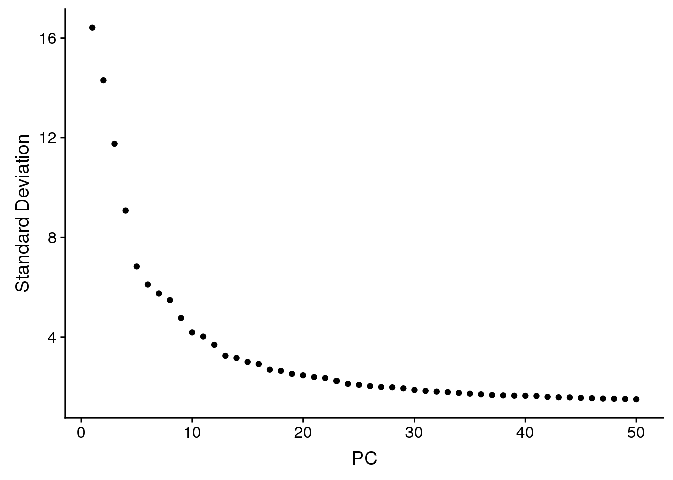
| Version | Author | Date |
|---|---|---|
| b502e30 | Belinda Phipson | 2019-07-05 |
VizDimLoadings(adult.integrated, dims = 1:4, reduction = "pca")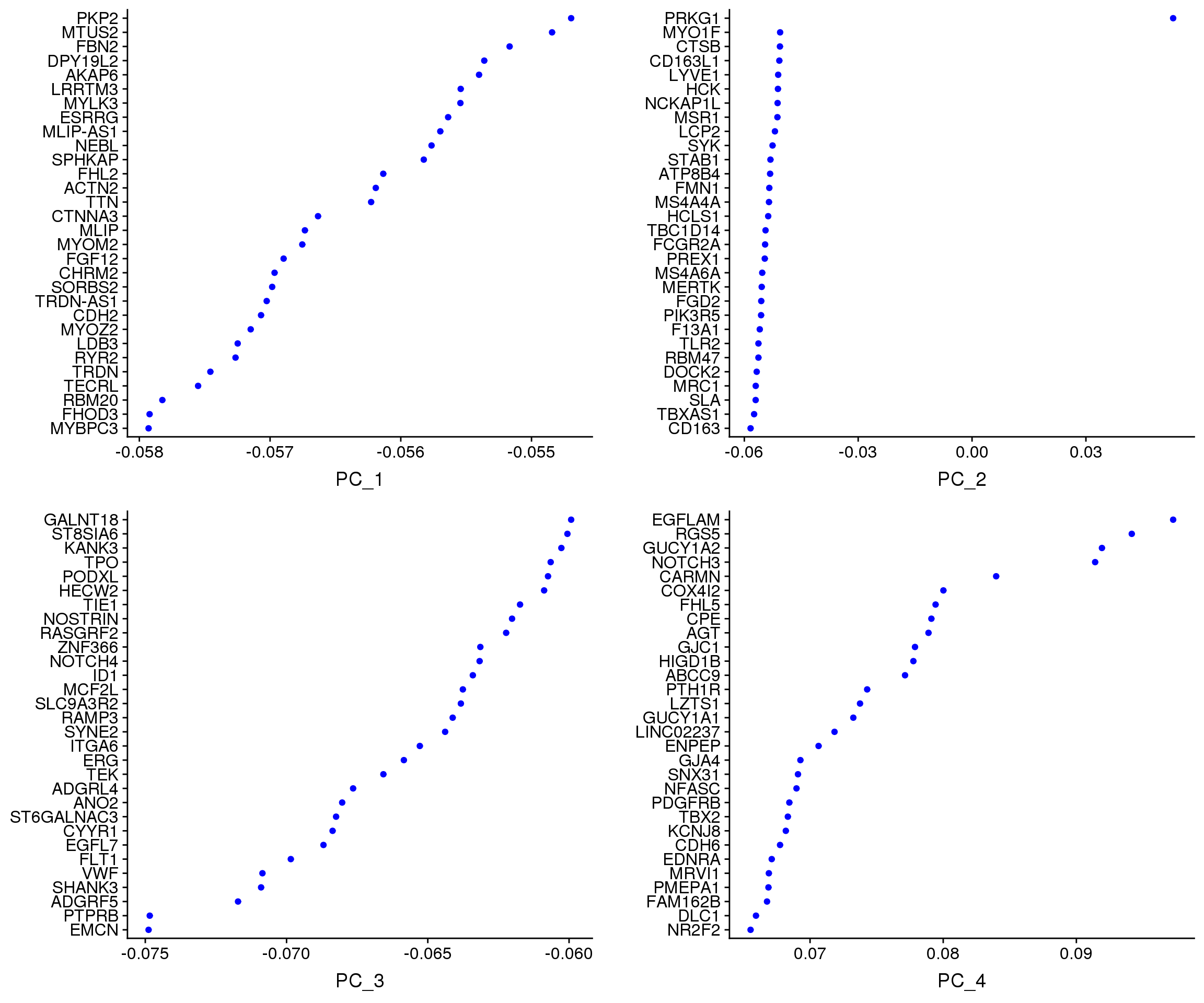
| Version | Author | Date |
|---|---|---|
| b502e30 | Belinda Phipson | 2019-07-05 |
DimPlot(adult.integrated, reduction = "pca",group.by="biorep")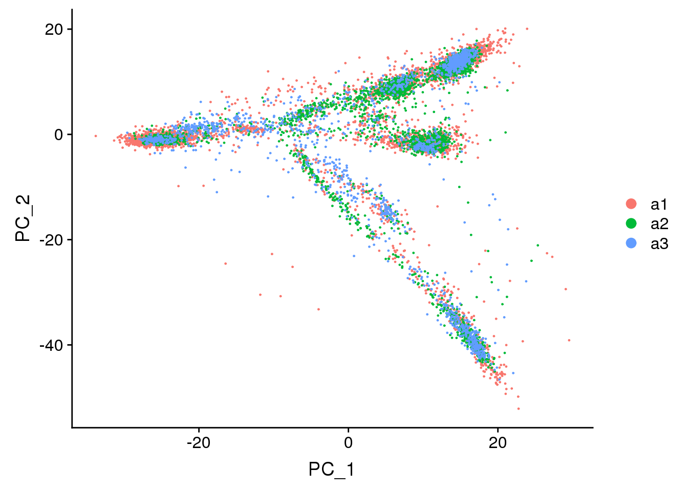
| Version | Author | Date |
|---|---|---|
| b502e30 | Belinda Phipson | 2019-07-05 |
DimPlot(adult.integrated, reduction = "pca",group.by="sex")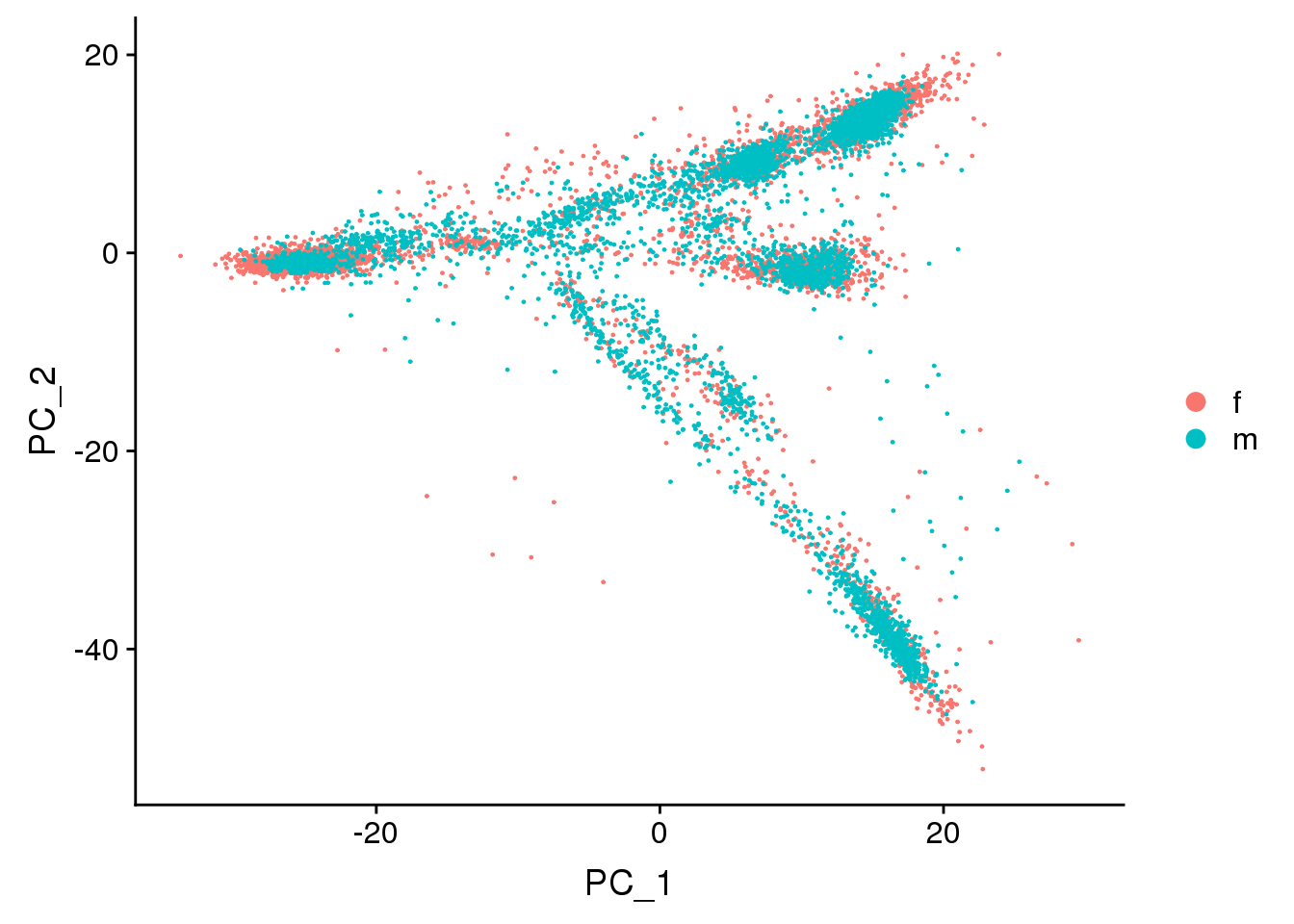
| Version | Author | Date |
|---|---|---|
| b502e30 | Belinda Phipson | 2019-07-05 |
DimPlot(adult.integrated, reduction = "pca",group.by="batch")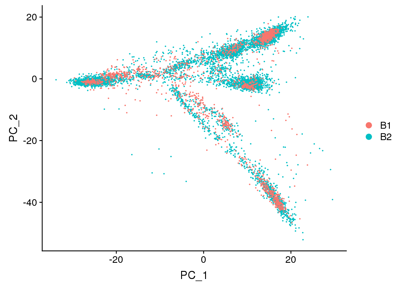
| Version | Author | Date |
|---|---|---|
| b502e30 | Belinda Phipson | 2019-07-05 |
DimHeatmap(adult.integrated, dims = 1:15, cells = 500, balanced = TRUE)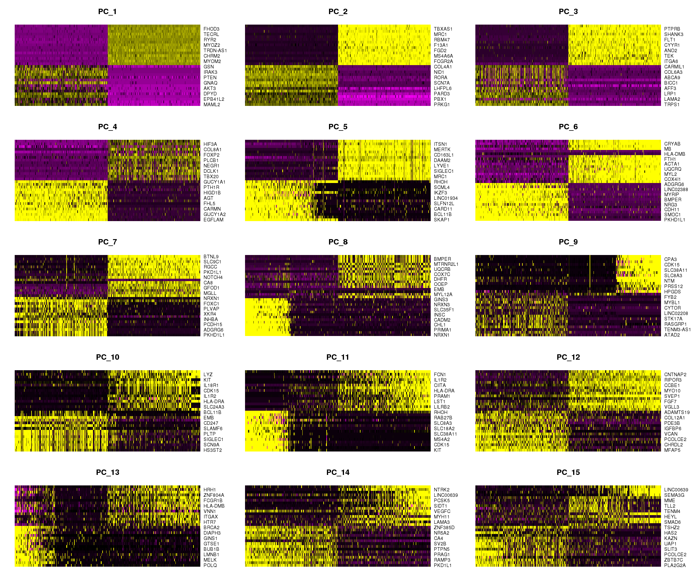
| Version | Author | Date |
|---|---|---|
| b502e30 | Belinda Phipson | 2019-07-05 |
DimHeatmap(adult.integrated, dims = 16:30, cells = 500, balanced = TRUE)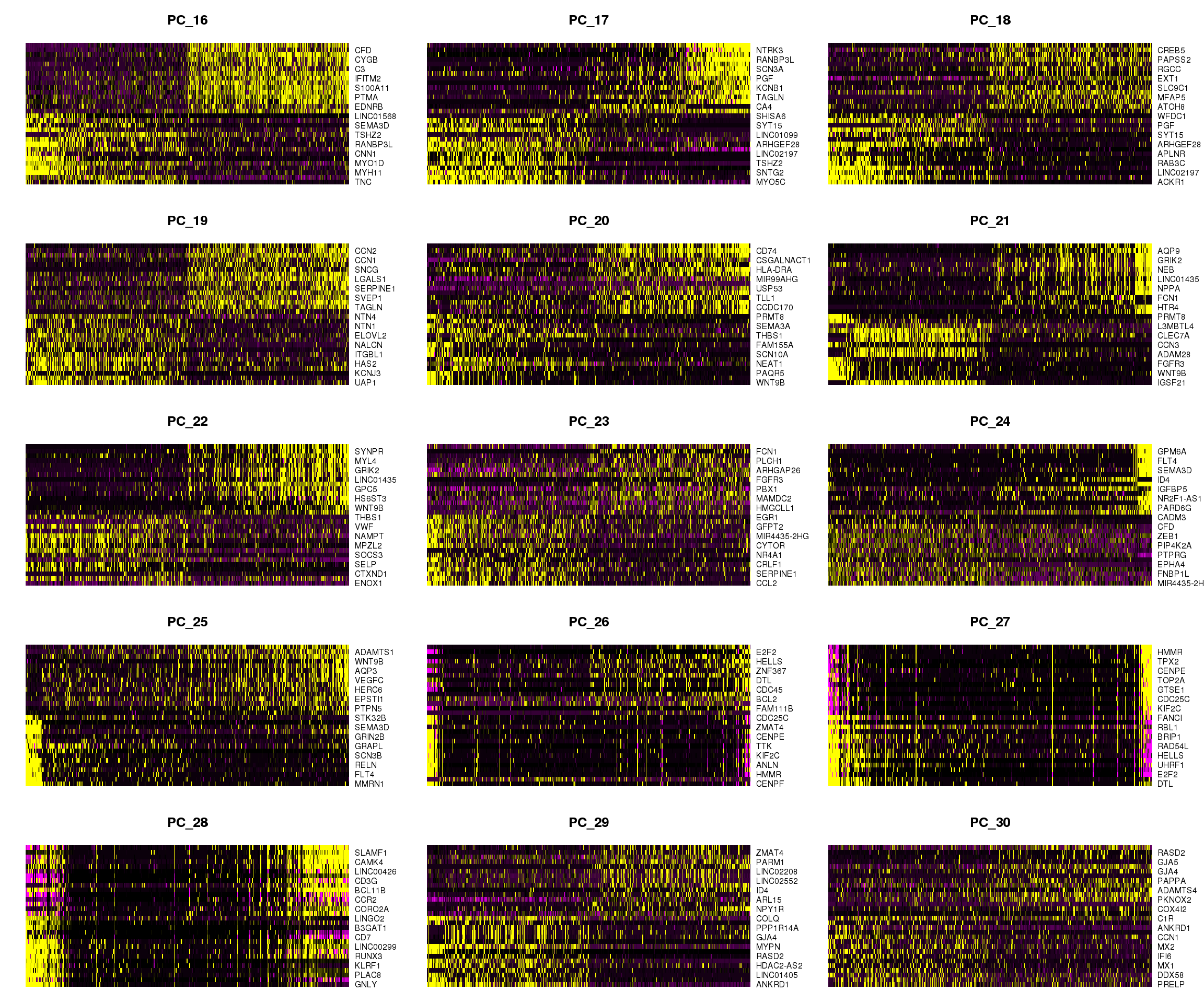
| Version | Author | Date |
|---|---|---|
| b502e30 | Belinda Phipson | 2019-07-05 |
Perform nearest neighbours clustering
adult.integrated <- FindNeighbors(adult.integrated, dims = 1:20)Computing nearest neighbor graphComputing SNNadult.integrated <- FindClusters(adult.integrated, resolution = 0.6)Modularity Optimizer version 1.3.0 by Ludo Waltman and Nees Jan van Eck
Number of nodes: 9416
Number of edges: 354612
Running Louvain algorithm...
Maximum modularity in 10 random starts: 0.9127
Number of communities: 21
Elapsed time: 0 secondstable(Idents(adult.integrated))
0 1 2 3 4 5 6 7 8 9 10 11 12 13 14
1845 1074 928 724 669 650 546 516 398 389 330 212 210 199 133
15 16 17 18 19 20
121 117 114 92 84 65 Visualisation with TSNE
set.seed(10)
adult.integrated <- RunTSNE(adult.integrated, reduction = "pca", dims = 1:20)pdf(file="./output/Figures/tsne-adultALL.pdf",width=10,height=8,onefile = FALSE)
DimPlot(adult.integrated, reduction = "tsne",label=TRUE,label.size = 6,pt.size = 0.5)+NoLegend()
dev.off()png
2 DimPlot(adult.integrated, reduction = "tsne",label=TRUE,label.size = 6)+NoLegend()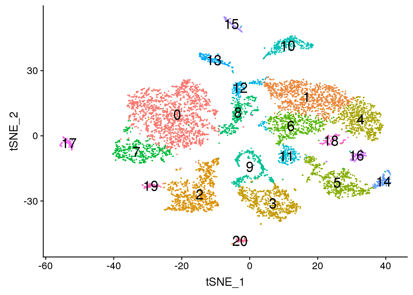
| Version | Author | Date |
|---|---|---|
| b502e30 | Belinda Phipson | 2019-07-05 |
DimPlot(adult.integrated, reduction = "tsne", split.by = "biorep",label=TRUE,label.size = 5)+NoLegend()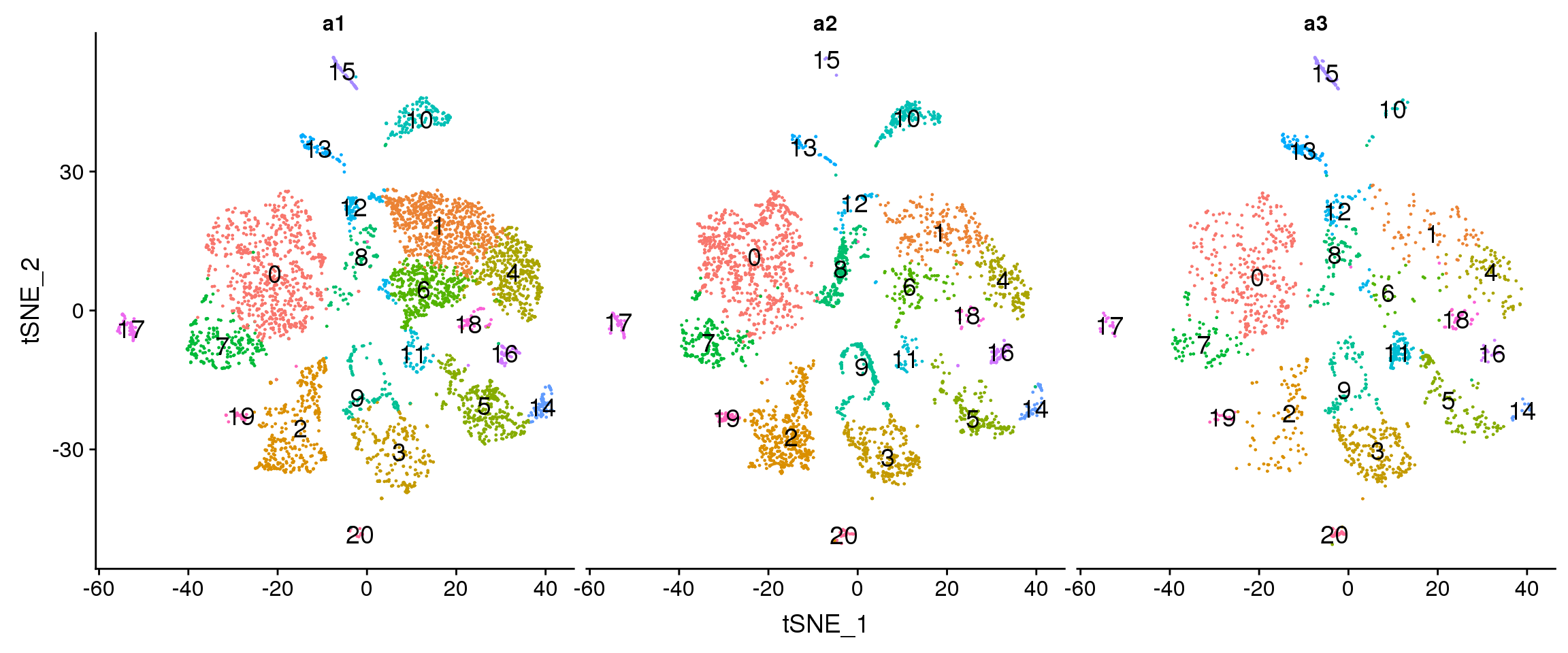
| Version | Author | Date |
|---|---|---|
| b502e30 | Belinda Phipson | 2019-07-05 |
DimPlot(adult.integrated, reduction = "tsne", split.by = "sex",label=TRUE,label.size = 5)+NoLegend()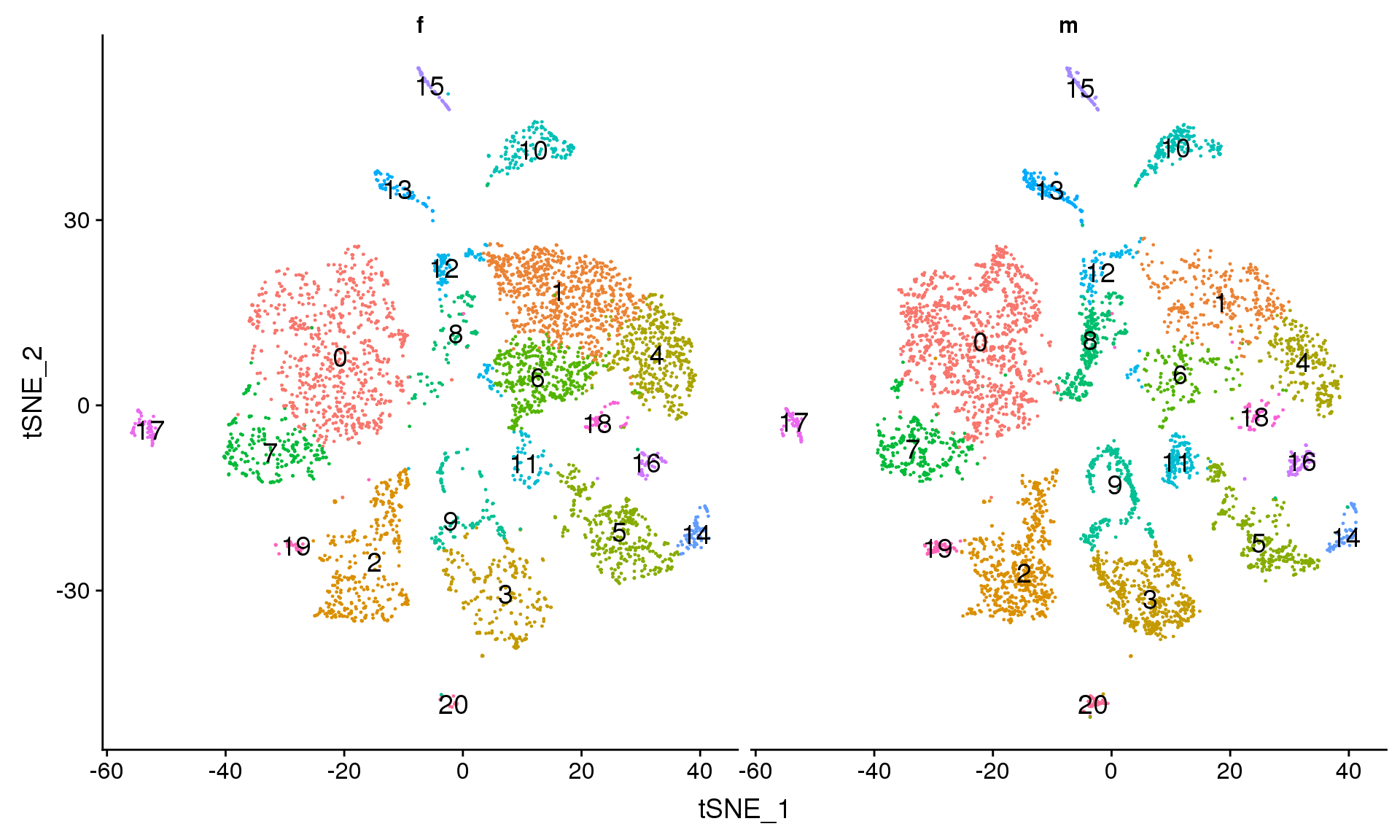
| Version | Author | Date |
|---|---|---|
| b502e30 | Belinda Phipson | 2019-07-05 |
DimPlot(adult.integrated, reduction = "tsne", group.by = "biorep")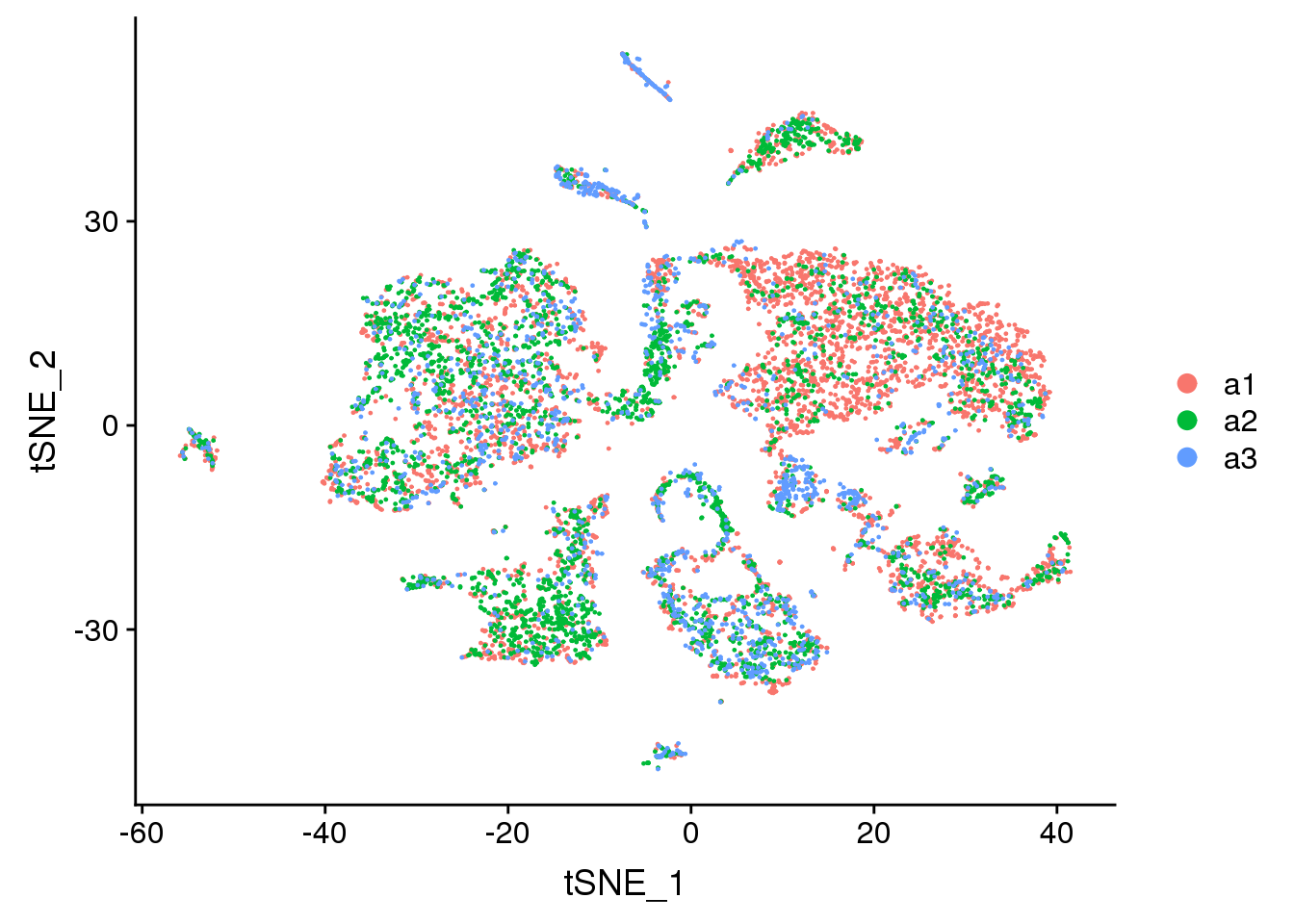
| Version | Author | Date |
|---|---|---|
| b502e30 | Belinda Phipson | 2019-07-05 |
DimPlot(adult.integrated, reduction = "tsne", group.by = "sex")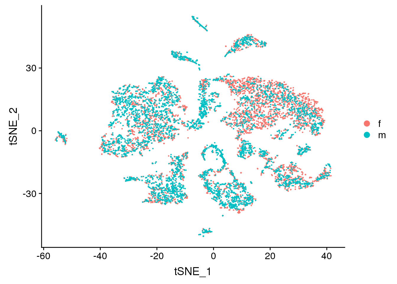
| Version | Author | Date |
|---|---|---|
| b502e30 | Belinda Phipson | 2019-07-05 |
DimPlot(adult.integrated, reduction = "tsne", group.by = "batch")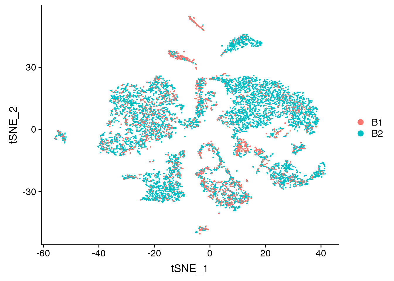
| Version | Author | Date |
|---|---|---|
| b502e30 | Belinda Phipson | 2019-07-05 |
#FeaturePlot(adult.integrated, features = c("XIST"))FeaturePlot(adult.integrated, features = c("TNNT2", "MYH6", "WT1", "PECAM1", "TBX3", "PDGFRA"), pt.size = 0.2,
ncol = 3)Warning: Found the following features in more than one assay, excluding the
default. We will not include these in the final dataframe: PDGFRAWarning in FetchData(object = object, vars = c(dims, "ident", features), :
The following requested variables were not found: PDGFRA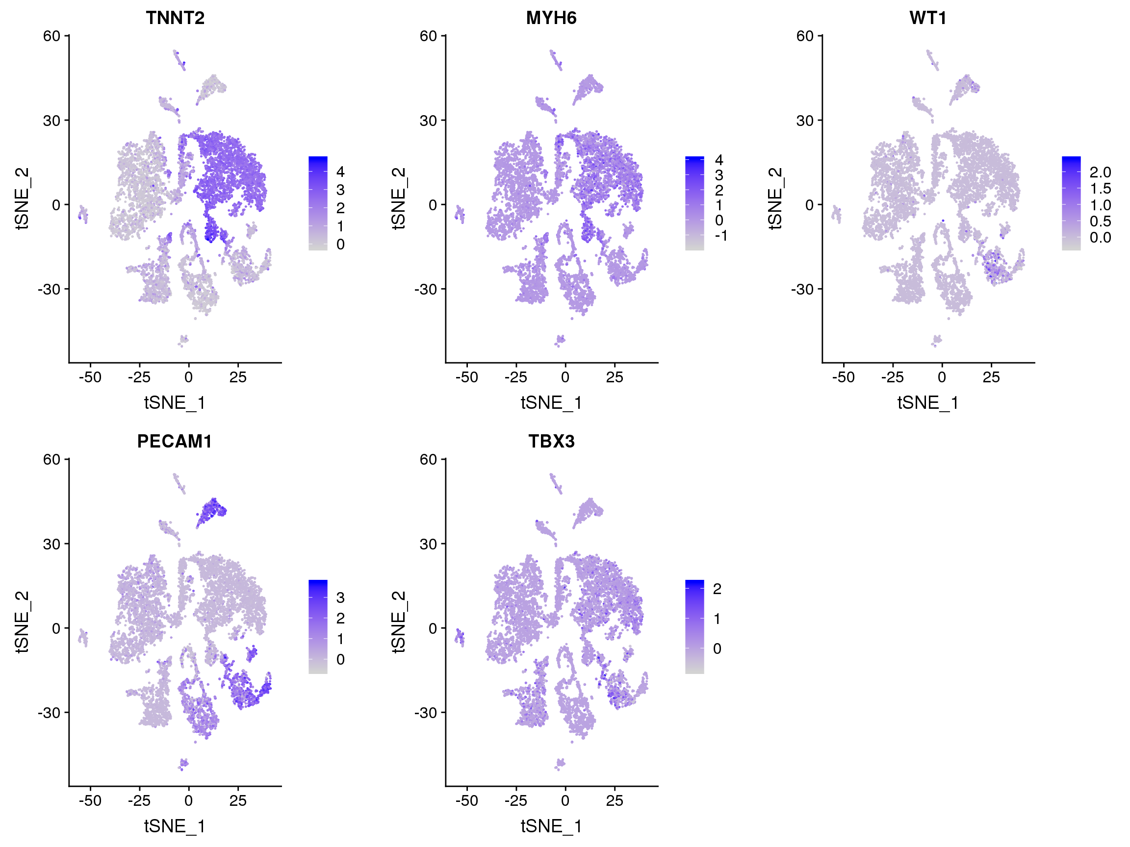
par(mfrow=c(1,1))
par(mar=c(4,4,2,2))
tab <- table(Idents(adult.integrated),adult@meta.data$biorep)
barplot(t(tab/rowSums(tab)),beside=TRUE,col=ggplotColors(3),legend=TRUE)
| Version | Author | Date |
|---|---|---|
| b502e30 | Belinda Phipson | 2019-07-05 |
Visualisation with clustree
clusres <- c(0.1,0.2,0.3,0.4,0.5,0.6,0.7,0.8,0.9,1,1.1,1.2)for(i in 1:length(clusres)){
adult.integrated <- FindClusters(adult.integrated,
resolution = clusres[i])
}Modularity Optimizer version 1.3.0 by Ludo Waltman and Nees Jan van Eck
Number of nodes: 9416
Number of edges: 354612
Running Louvain algorithm...
Maximum modularity in 10 random starts: 0.9778
Number of communities: 10
Elapsed time: 0 seconds
Modularity Optimizer version 1.3.0 by Ludo Waltman and Nees Jan van Eck
Number of nodes: 9416
Number of edges: 354612
Running Louvain algorithm...
Maximum modularity in 10 random starts: 0.9616
Number of communities: 13
Elapsed time: 0 seconds
Modularity Optimizer version 1.3.0 by Ludo Waltman and Nees Jan van Eck
Number of nodes: 9416
Number of edges: 354612
Running Louvain algorithm...
Maximum modularity in 10 random starts: 0.9463
Number of communities: 15
Elapsed time: 0 seconds
Modularity Optimizer version 1.3.0 by Ludo Waltman and Nees Jan van Eck
Number of nodes: 9416
Number of edges: 354612
Running Louvain algorithm...
Maximum modularity in 10 random starts: 0.9331
Number of communities: 19
Elapsed time: 0 seconds
Modularity Optimizer version 1.3.0 by Ludo Waltman and Nees Jan van Eck
Number of nodes: 9416
Number of edges: 354612
Running Louvain algorithm...
Maximum modularity in 10 random starts: 0.9222
Number of communities: 20
Elapsed time: 1 seconds
Modularity Optimizer version 1.3.0 by Ludo Waltman and Nees Jan van Eck

Number of nodes: 9416
Number of edges: 354612

Running Louvain algorithm...
Maximum modularity in 10 random starts: 0.9127
Number of communities: 21
Elapsed time: 0 seconds
Modularity Optimizer version 1.3.0 by Ludo Waltman and Nees Jan van Eck
Number of nodes: 9416
Number of edges: 354612
Running Louvain algorithm...
Maximum modularity in 10 random starts: 0.9048
Number of communities: 23
Elapsed time: 0 seconds
Modularity Optimizer version 1.3.0 by Ludo Waltman and Nees Jan van Eck
Number of nodes: 9416
Number of edges: 354612
Running Louvain algorithm...
Maximum modularity in 10 random starts: 0.8986
Number of communities: 24
Elapsed time: 0 seconds
Modularity Optimizer version 1.3.0 by Ludo Waltman and Nees Jan van Eck
Number of nodes: 9416
Number of edges: 354612
Running Louvain algorithm...
Maximum modularity in 10 random starts: 0.8930
Number of communities: 26
Elapsed time: 0 seconds
Modularity Optimizer version 1.3.0 by Ludo Waltman and Nees Jan van Eck
Number of nodes: 9416
Number of edges: 354612
Running Louvain algorithm...
Maximum modularity in 10 random starts: 0.8872
Number of communities: 27
Elapsed time: 0 seconds
Modularity Optimizer version 1.3.0 by Ludo Waltman and Nees Jan van Eck
Number of nodes: 9416
Number of edges: 354612
Running Louvain algorithm...
Maximum modularity in 10 random starts: 0.8816
Number of communities: 27
Elapsed time: 0 seconds
Modularity Optimizer version 1.3.0 by Ludo Waltman and Nees Jan van Eck
Number of nodes: 9416
Number of edges: 354612
Running Louvain algorithm...
Maximum modularity in 10 random starts: 0.8757
Number of communities: 27
Elapsed time: 0 secondspct.male <- function(x) {mean(x=="m")}
pct.female <- function(x) {mean(x=="f")}
biorep1 <- function(x) {mean(x=="a1")}
biorep2 <- function(x) {mean(x=="a2")}
biorep3 <- function(x) {mean(x=="a3")}clustree(adult.integrated, prefix = "integrated_snn_res.")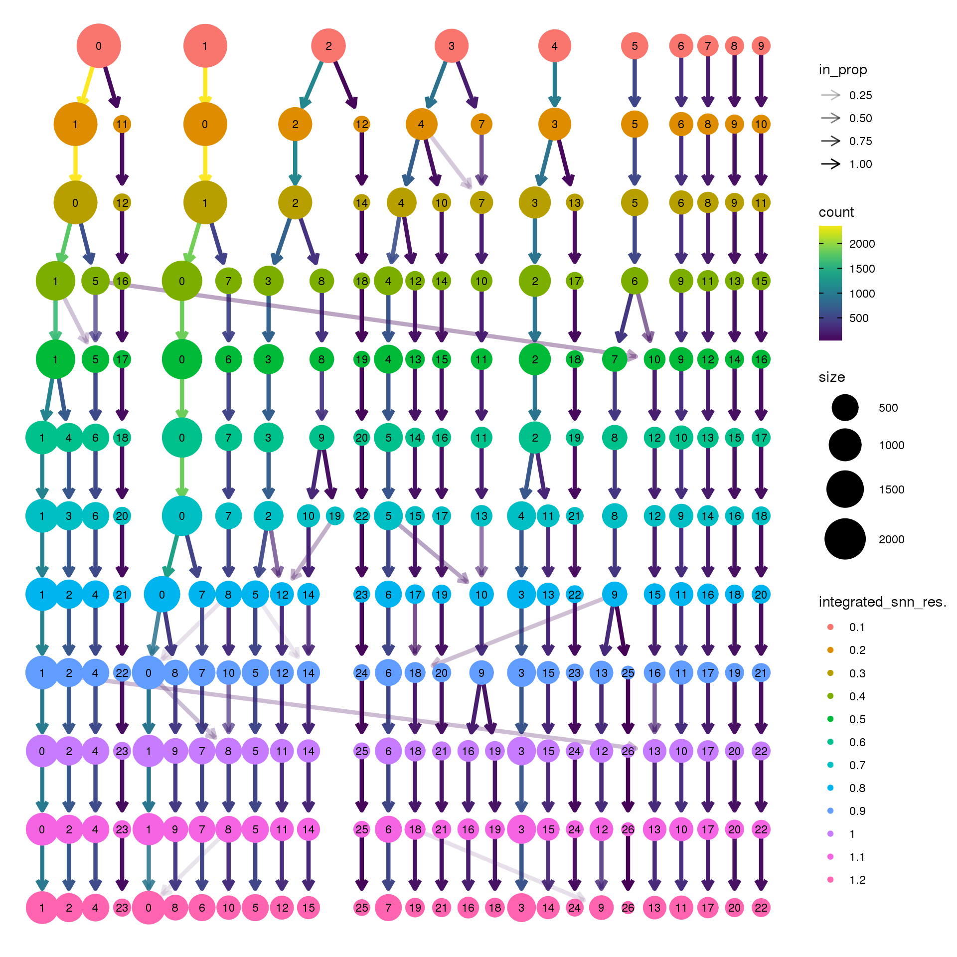
clustree(adult.integrated, prefix = "integrated_snn_res.",
node_colour = "biorep", node_colour_aggr = "biorep1",assay="RNA")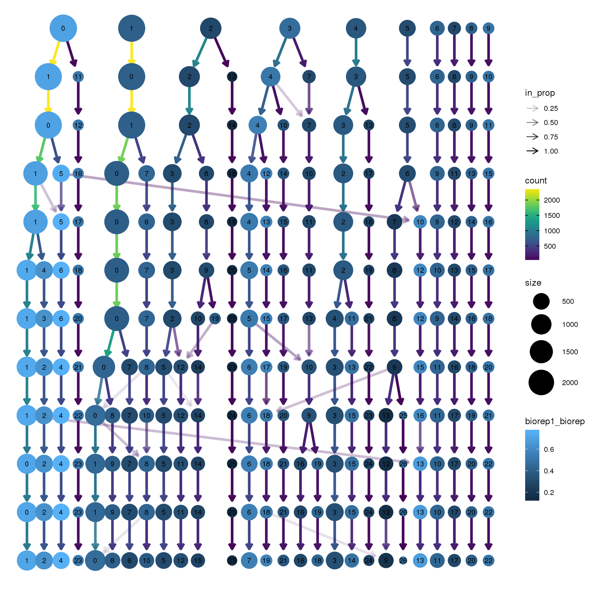
| Version | Author | Date |
|---|---|---|
| b502e30 | Belinda Phipson | 2019-07-05 |
clustree(adult.integrated, prefix = "integrated_snn_res.",
node_colour = "biorep", node_colour_aggr = "biorep2",assay="RNA")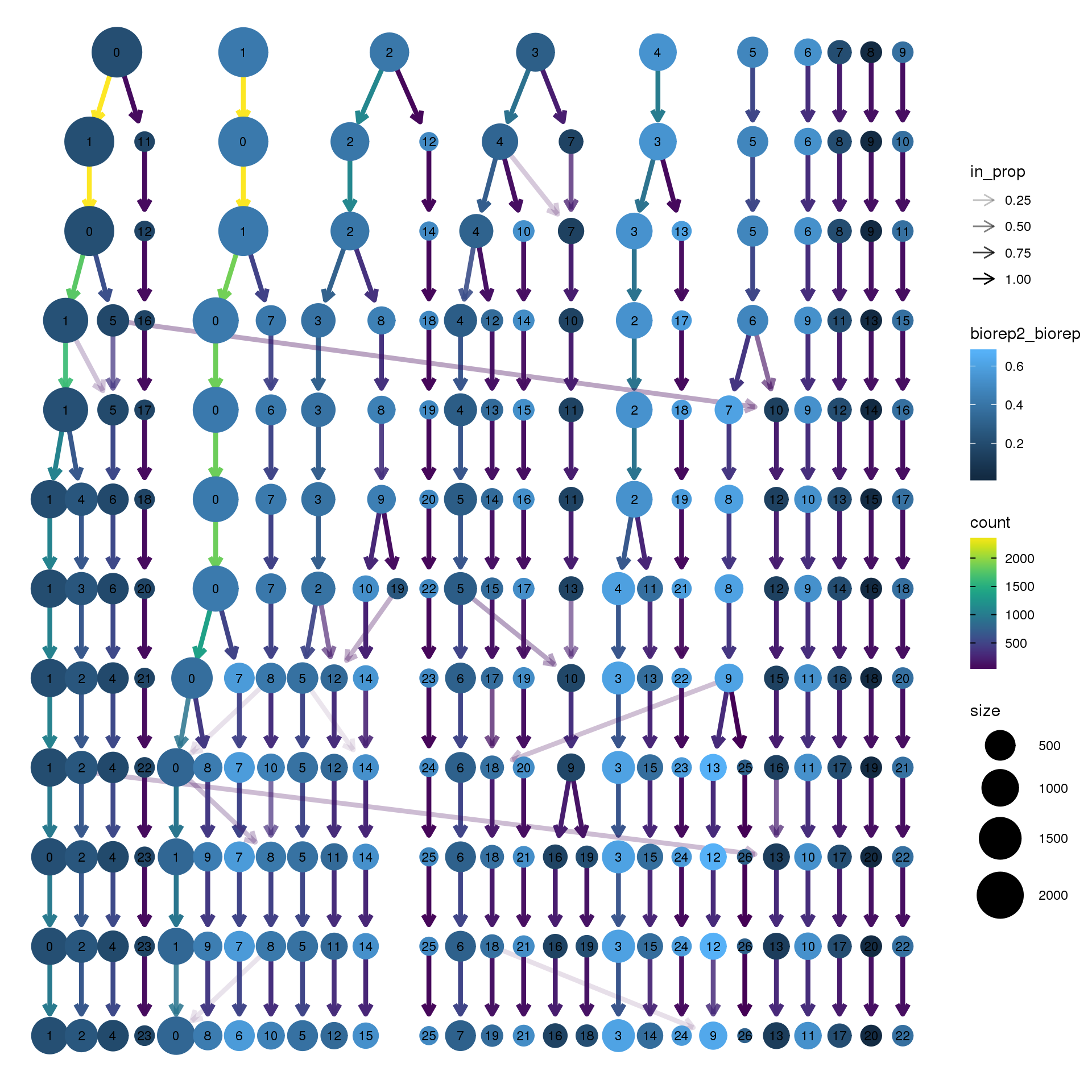
| Version | Author | Date |
|---|---|---|
| b502e30 | Belinda Phipson | 2019-07-05 |
clustree(adult.integrated, prefix = "integrated_snn_res.",
node_colour = "biorep", node_colour_aggr = "biorep3",assay="RNA")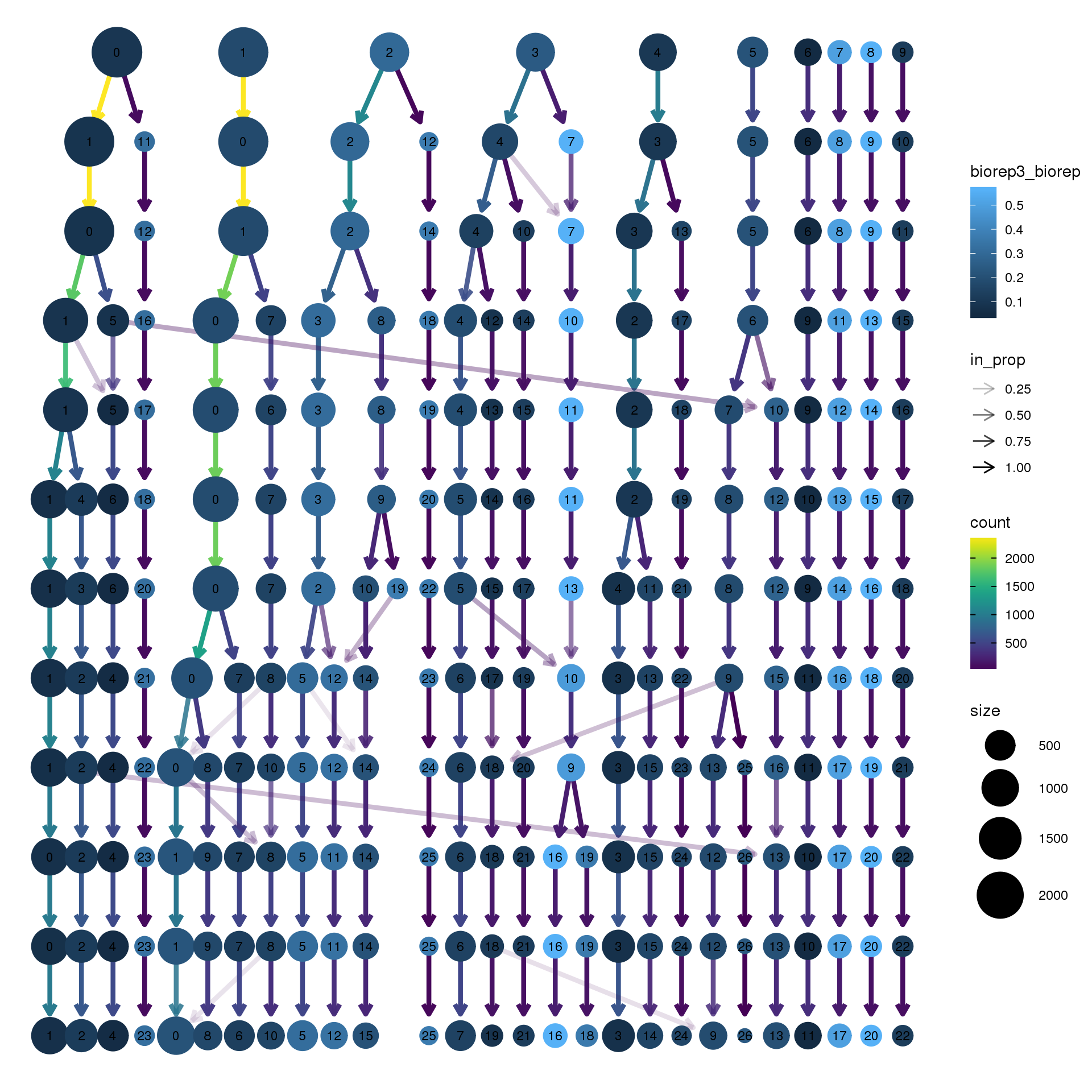
| Version | Author | Date |
|---|---|---|
| b502e30 | Belinda Phipson | 2019-07-05 |
clustree(adult.integrated, prefix = "integrated_snn_res.",
node_colour = "sex", node_colour_aggr = "pct.female",assay="RNA")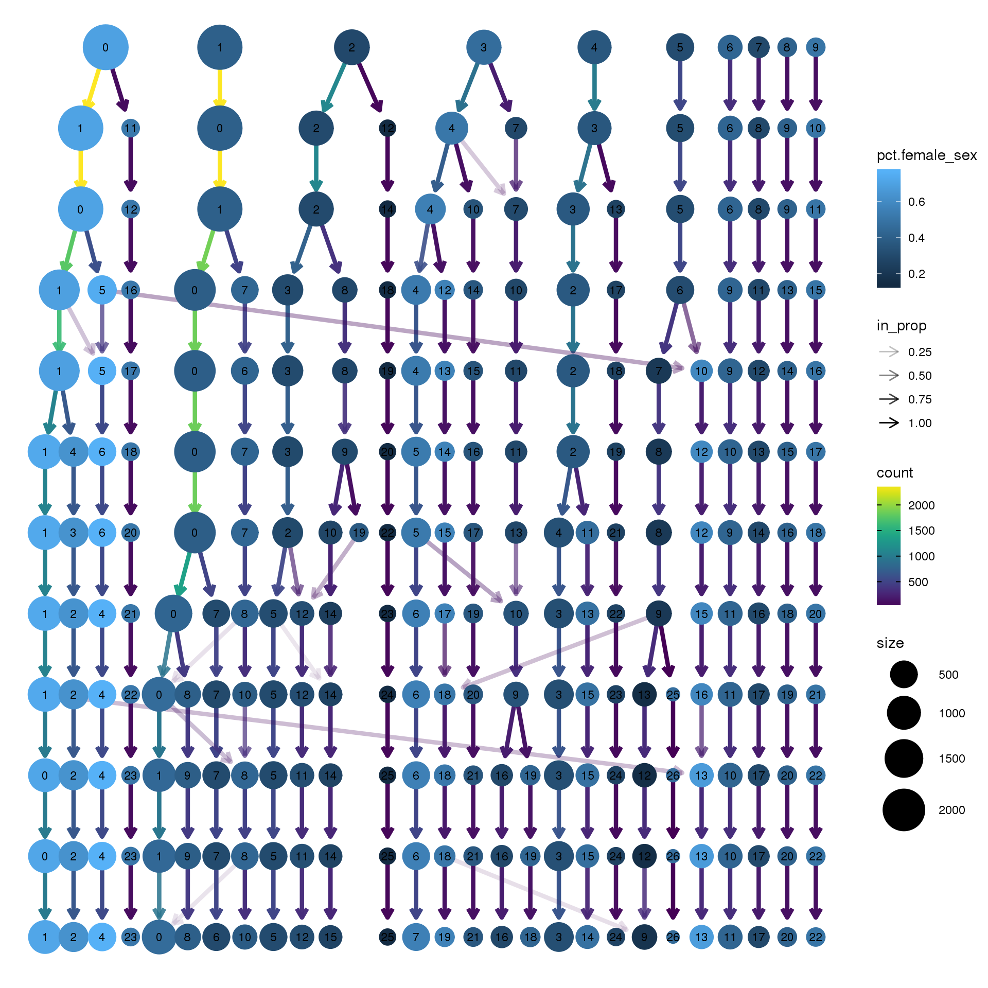
| Version | Author | Date |
|---|---|---|
| b502e30 | Belinda Phipson | 2019-07-05 |
clustree(adult.integrated, prefix = "integrated_snn_res.",
node_colour = "sex", node_colour_aggr = "pct.male",assay="RNA")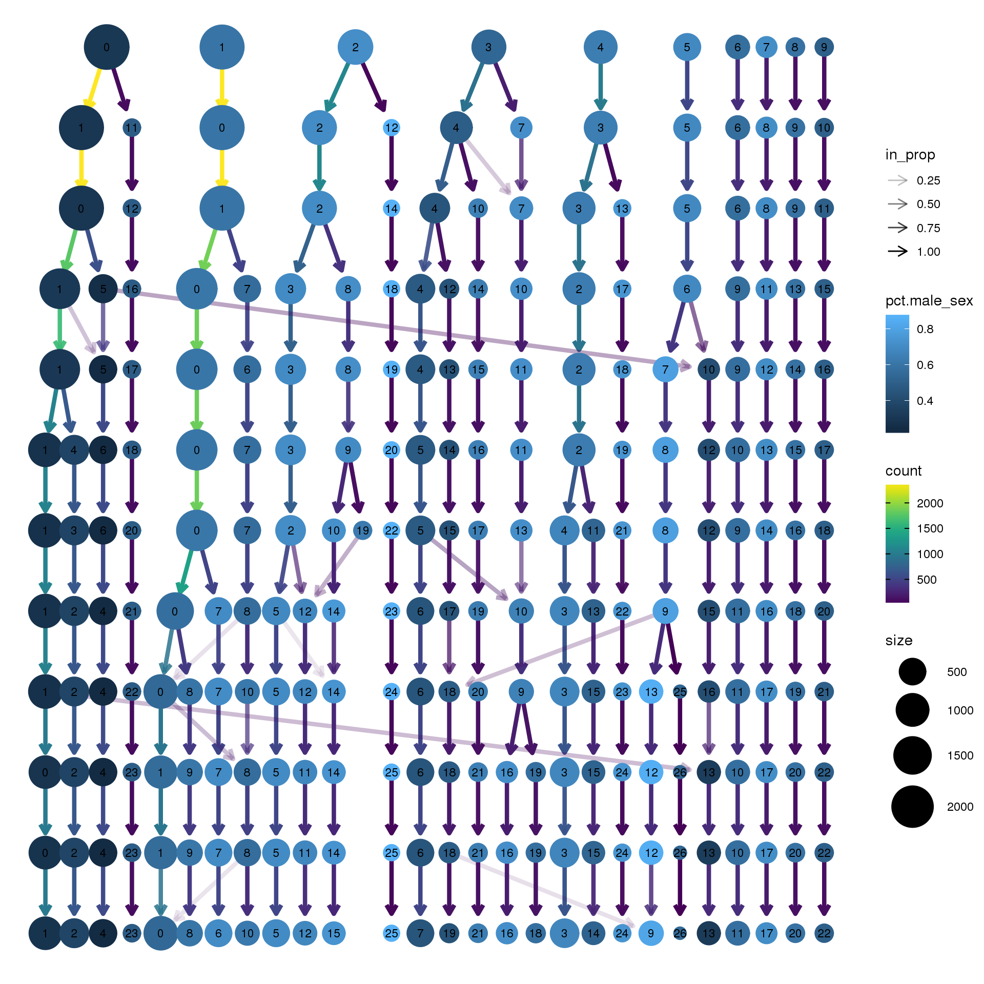
| Version | Author | Date |
|---|---|---|
| b502e30 | Belinda Phipson | 2019-07-05 |
#clustree(adult.integrated, prefix = "integrated_snn_res.",
# node_colour = "XIST", node_colour_aggr = "median",
# assay="RNA")clustree(adult.integrated, prefix = "integrated_snn_res.",
node_colour = "TNNT2", node_colour_aggr = "median",
assay="RNA")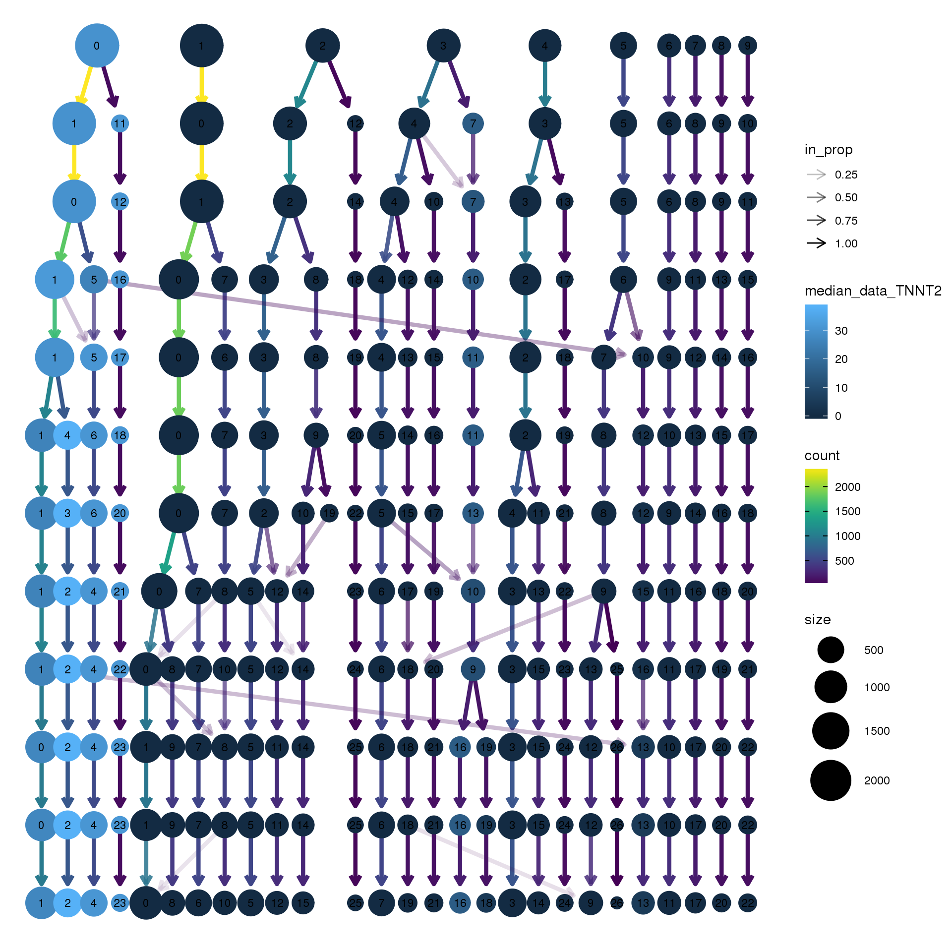
Save Seurat object
DefaultAssay(adult.integrated) <- "RNA"
Idents(adult.integrated) <- adult.integrated$integrated_snn_res.0.6saveRDS(adult.integrated,file="./output/RDataObjects/adult-int.Rds")Find Markers
par(mfrow=c(1,1))
par(mar=c(4,4,2,2))
tab <- table(Idents(adult.integrated),adult@meta.data$biorep)
barplot(t(tab/rowSums(tab)),beside=TRUE,col=ggplotColors(3),legend=TRUE)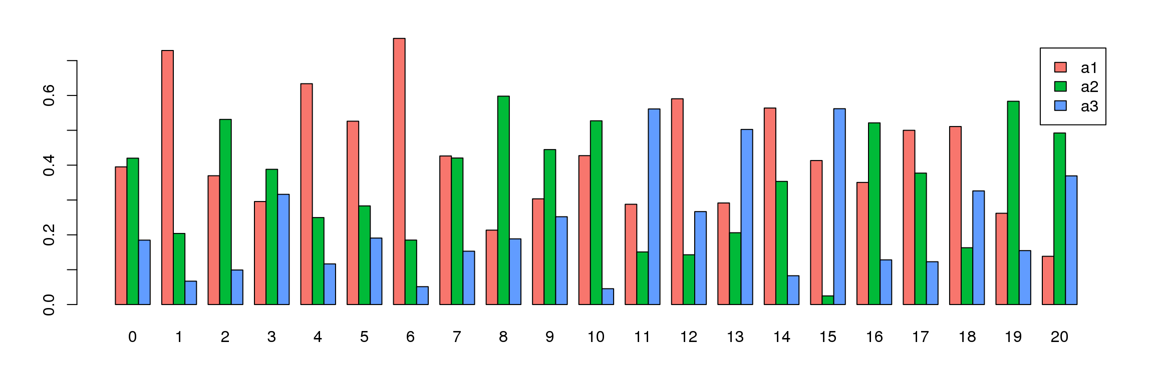
#adultmarkers <- FindAllMarkers(adult.integrated, only.pos = TRUE, min.pct = 0.25, logfc.threshold = 0.25)
# Limma-trend for DE

y.adult <- DGEList(alla.keep)

logcounts <- normCounts(y.adult,log=TRUE,prior.count=0.5)

#logcounts.n <- normalizeBetweenArrays(logcounts, method = "cyclicloess")

maxclust <- length(levels(Idents(adult.integrated)))-1

grp <- paste("c",Idents(adult.integrated),sep = "")
grp <- factor(grp,levels = paste("c",0:maxclust,sep=""))

design <- model.matrix(~0+grp)
colnames(design) <- levels(grp)

mycont <- matrix(NA,ncol=length(levels(grp)),nrow=length(levels(grp)))
rownames(mycont)<-colnames(mycont)<-levels(grp)
diag(mycont)<-1
mycont[upper.tri(mycont)]<- -1/(length(levels(factor(grp)))-1)
mycont[lower.tri(mycont)]<- -1/(length(levels(factor(grp)))-1)

fit <- lmFit(logcounts,design)
fit.cont <- contrasts.fit(fit,contrasts=mycont)
fit.cont <- eBayes(fit.cont,trend=TRUE,robust=TRUE)

fit.cont$genes <- ann.keep

summary(decideTests(fit.cont))
c0 c1 c2 c3 c4 c5 c6 c7 c8 c9 c10
Down 4054 5600 5412 5159 4219 5439 4471 3932 11588 8258 3068
NotSig 5681 6449 8196 7127 6674 8832 7943 8974 5553 7557 10562
Up 7811 5497 3938 5260 6653 3275 5132 4640 405 1731 3916
c11 c12 c13 c14 c15 c16 c17 c18 c19 c20
Down 8406 9999 4755 2221 6995 2188 2672 162 1735 1384
NotSig 7542 7129 10254 12838 9474 13024 12804 12408 14126 11703
Up 1598 418 2537 2487 1077 2334 2070 4976 1685 4459treat <- treat(fit.cont,lfc=0.5)
dt <- decideTests(treat)
summary(dt) c0 c1 c2 c3 c4 c5 c6 c7 c8 c9 c10
Down 314 427 413 572 310 378 364 302 1378 782 285
NotSig 16333 16128 16480 15789 15994 16508 16220 16495 16107 16446 16609
Up 899 991 653 1185 1242 660 962 749 61 318 652
c11 c12 c13 c14 c15 c16 c17 c18 c19 c20
Down 1412 1232 720 241 801 253 306 0 156 222
NotSig 15716 16217 16247 16735 16427 16663 16696 16877 16928 16191
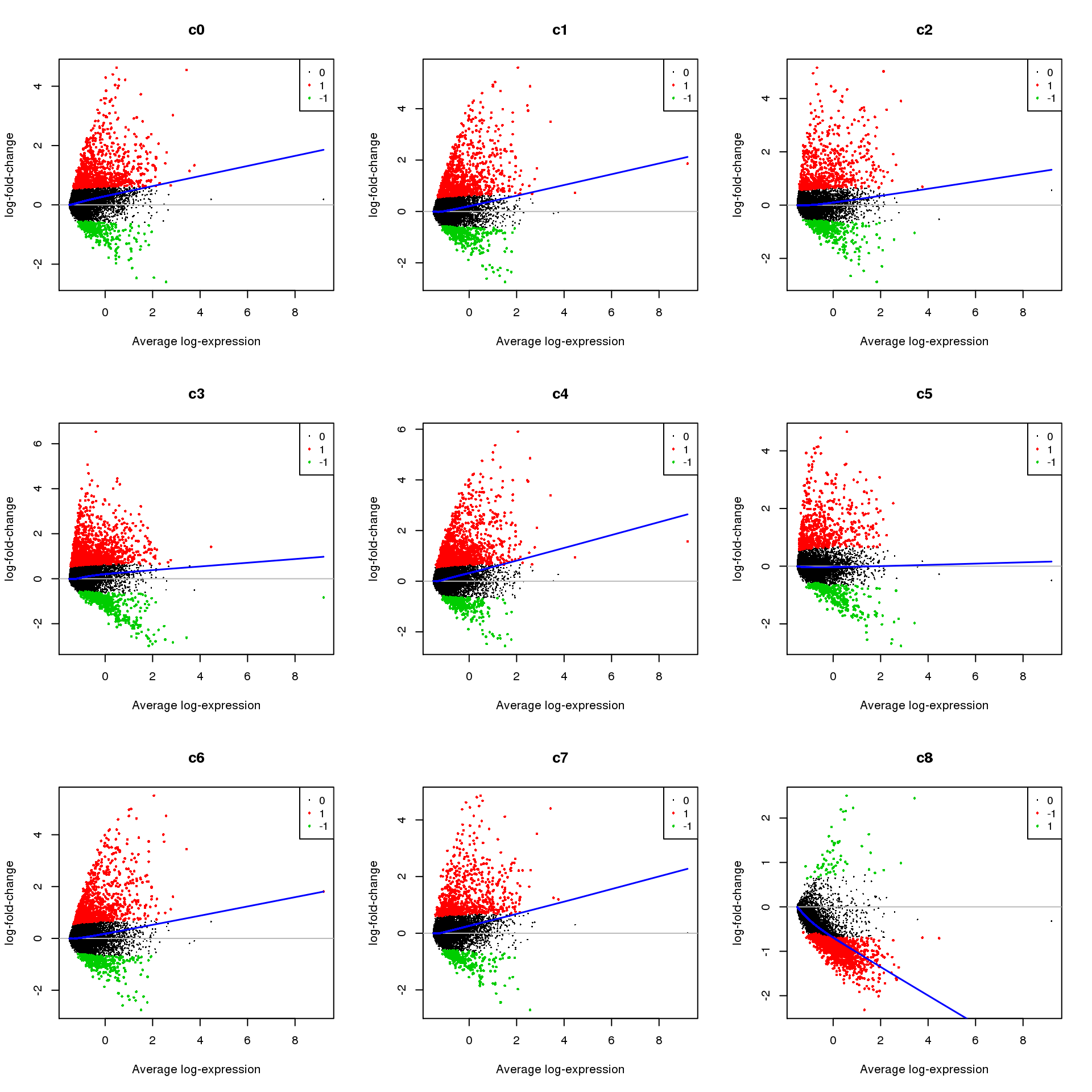
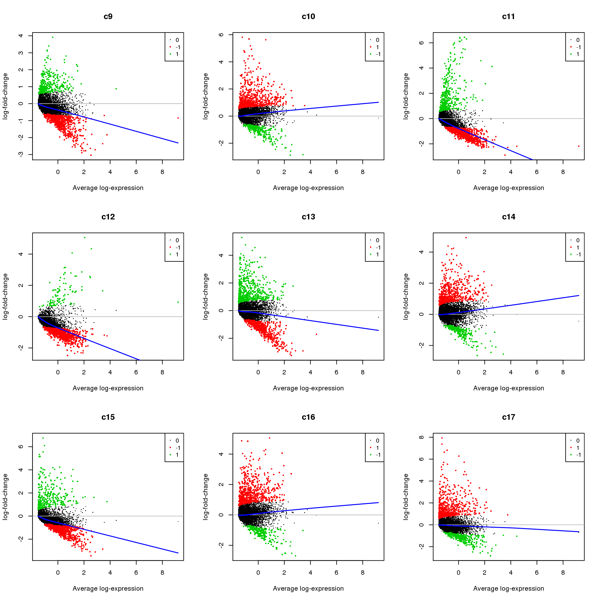
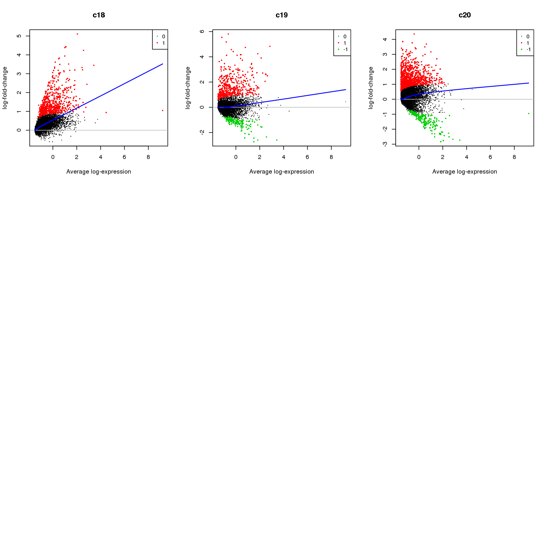
Up 418 97 579 570 318 630 544 669 462 1133par(mfrow=c(3,3))
for(i in 1:ncol(mycont)){
plotMD(treat,coef=i,status = dt[,i],hl.cex=0.5)
abline(h=0,col=colours()[c(226)])
lines(lowess(treat$Amean,treat$coefficients[,i]),lwd=1.5,col=4)
}
| Version | Author | Date |
|---|---|---|
| b502e30 | Belinda Phipson | 2019-07-05 |
Write out marker genes for each cluster
#write.csv(adultmarkers,file="./output/AllAdult-clustermarkers.csv")

contnames <- colnames(mycont)

for(i in 1:length(contnames)){
  topsig <- topTreat(treat,coef=i,n=Inf,p.value=0.05)
  write.csv(topsig[topsig$logFC>0,],file=paste("./output/MarkerAnalysis/Adult/Up-Cluster-",contnames[i],".csv",sep=""))
  write.csv(topGO(goana(de=topsig$ENTREZID[topsig$logFC>0],universe=treat$genes$ENTREZID,species="Hs"),number=50),
            file=paste("./output/MarkerAnalysis/Adult/GO-Cluster-",contnames[i],".csv",sep=""))

}
Heatmap of pre-defined heart cell type markers
hm <- read.delim("./data/heart-markers-long.txt",stringsAsFactors = FALSE)
hgene <- toupper(hm$Gene)
hgene <- unique(hgene)

m <- match(hgene,rownames(logcounts))
m <- m[!is.na(m)]

sam <- factor(adult.integrated$biorep)
newgrp <- paste(grp,sam,sep=".")
newgrp <- factor(newgrp,levels=paste(rep(levels(grp),each=3),levels(sam),sep="."))
o <-order(newgrp)

annot <- data.frame(CellType=grp,Sample=sam,NewGroup=newgrp)

mycelltypes <- hm$Celltype[match(rownames(logcounts)[m],toupper(hm$Gene))]
mycelltypes <- factor(mycelltypes)


myColors <- list(Clust=NA,Sample=NA,Celltypes=NA)
myColors$Clust<-sample(ggplotColors(length(levels(grp))),length(levels(grp)))
names(myColors$Clust)<-levels(grp)
myColors$Sample <- brewer.pal(3, "Set1")
names(myColors$Sample) <- levels(sam)
myColors$Celltypes <- ggplotColors(length(levels(mycelltypes)))
names(myColors$Celltypes) <- levels(mycelltypes)

mygenes <- rownames(logcounts)[m]
mygenelab <- paste(mygenes,mycelltypes,sep="_")
par(mfrow=c(1,1))
pdf(file="./output/Figures/adult-heatmap-hmarkers.pdf",width=20,height=15,onefile = FALSE)
aheatmap(logcounts[m,o],Rowv=NA,Colv=NA,labRow=mygenelab,labCol=NA,
annCol=list(Clust=grp[o],Sample=sam[o]),
# annRow = list(Celltypes=mycelltypes),
annColors = myColors,
fontsize=16,color="-RdYlBu")
dev.off()png
2 Summarise expression across cells
sumexpr <- matrix(NA,nrow=nrow(logcounts),ncol=length(levels(newgrp)))
rownames(sumexpr) <- rownames(logcounts)
colnames(sumexpr) <- levels(newgrp)

for(i in 1:nrow(sumexpr)){
  sumexpr[i,] <- tapply(logcounts[i,],newgrp,median)
}
par(mfrow=c(1,1))
clust <- rep(levels(grp),each=3)
samps <- rep(levels(sam),length(levels(grp)))
pdf(file="./output/Figures/adult-heatmap-hmarkers-summarised.pdf",width=20,height=15,onefile = FALSE)
aheatmap(sumexpr[m,],Rowv = NA,Colv = NA, labRow = mygenelab,
annCol=list(Clust=clust,Sample=samps),
# annRow=list(Celltypes=mycelltypes),
annColors=myColors,
fontsize=14,color="-RdYlBu")
dev.off()png
2 aheatmap(sumexpr[m,],Rowv = NA,Colv = NA, labRow = mygenelab,
annCol=list(Clust=clust,Sample=samps),
# annRow=list(Celltypes=mycelltypes),
annColors=myColors,
fontsize=12,color="-RdYlBu")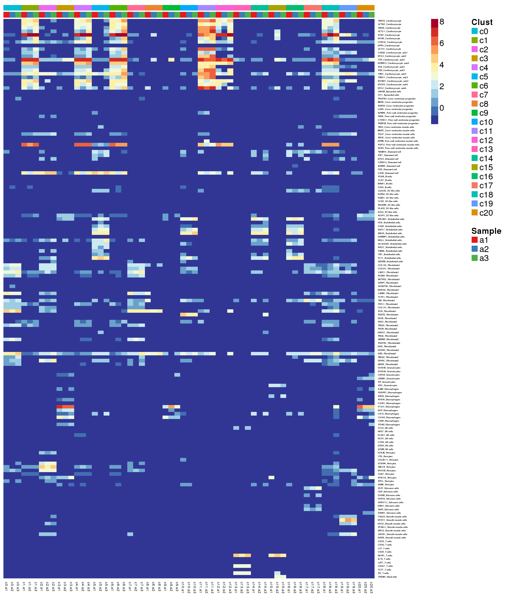
sig.genes <- gene.label <- vector("list", length(levels(grp)))
for(i in 1:length(sig.genes)){
  top <- topTreat(treat,coef=i,n=200)
  sig.genes[[i]] <- rownames(top)[top$logFC>0][1:5]
  gene.label[[i]] <- paste(rownames(top)[top$logFC>0][1:5],levels(grp)[i],sep="-")
}

csig <- unlist(sig.genes)
genes <- unlist(gene.label)

pdf(file="./output/Figures/adult-heatmap-siggenes-summarised.pdf",width=20,height=15,onefile = FALSE)
aheatmap(sumexpr[csig,],Rowv = NA,Colv = NA, labRow = genes,
         annCol=list(Clust=clust,Sample=samps),
         annColors=myColors,
         fontsize=16,color="-RdYlBu",
         scale="none")
dev.off()
png
2 aheatmap(sumexpr[csig,],Rowv = NA,Colv = NA, labRow = genes,
annCol=list(Clust=clust,Sample=samps),
annColors=myColors,
fontsize=16,color="-RdYlBu",
scale="none")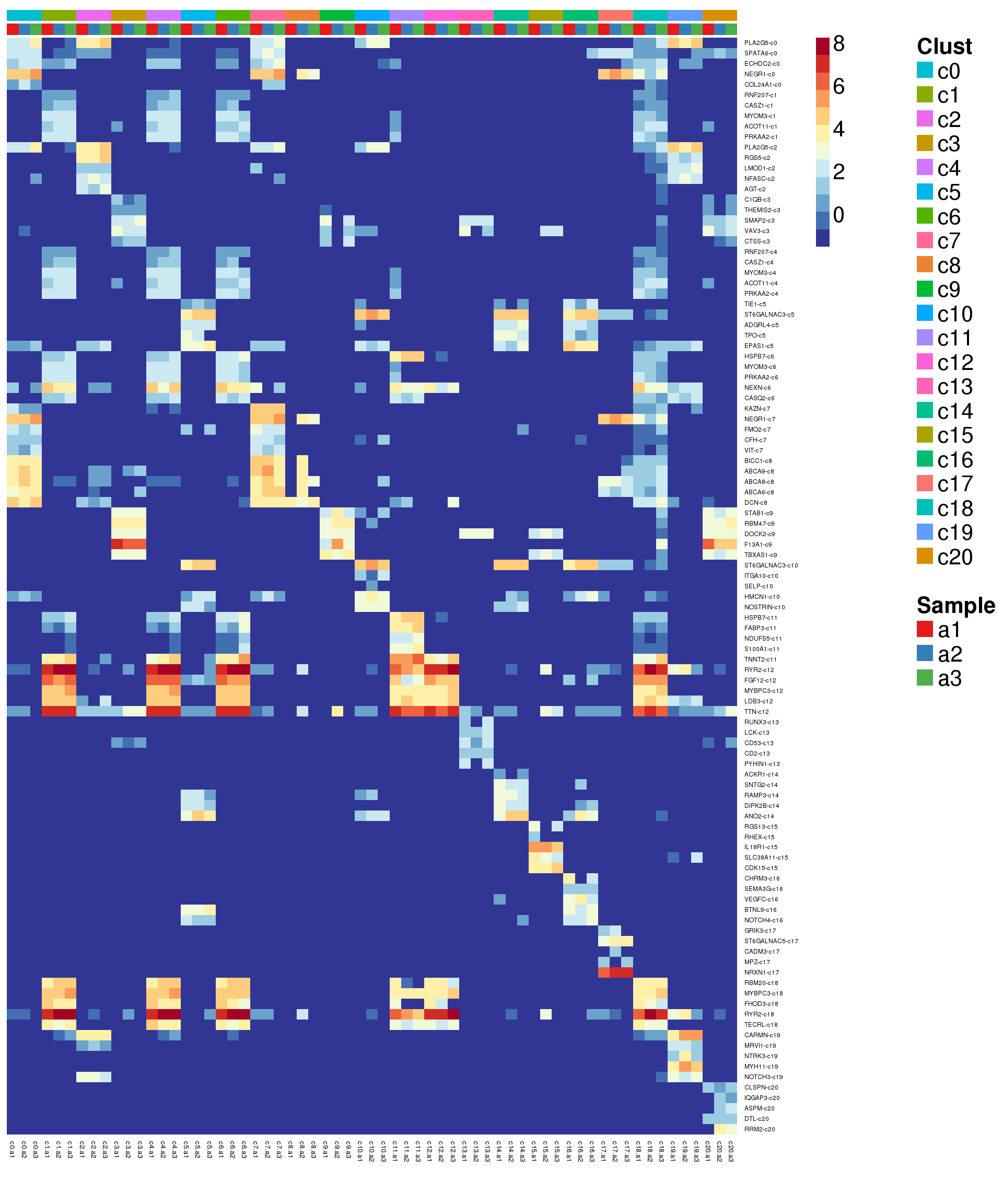
Try annotate clusters based on fetal cell types
# This loads a list object called sig.genes.gst
load(file="./data/gstlist-fetal.Rdata")

expr.score <- matrix(NA,nrow=length(sig.genes.gst),ncol=length(levels(newgrp)))
colnames(expr.score) <- levels(newgrp)
rownames(expr.score) <- names(sig.genes.gst)

specialm <- lapply(sig.genes.gst,function(x) match(x,rownames(sumexpr))[!is.na(match(x,rownames(sumexpr)))])

for(i in 1:nrow(expr.score)){
  expr.score[i,] <- colMedians(sumexpr[specialm[[i]],])
}

pdf(file="./output/Figures/heatmap-match-fetal-adult-medians.pdf",width=20,height=15,onefile = FALSE)
aheatmap(expr.score,
         Rowv = NA,Colv = NA,
         labRow = rownames(expr.score),
         annCol=list(Clust=clust,Sample=samps),
         annColors=myColors,
         fontsize=16,color="-RdYlBu",
         scale="none")
dev.off()
png
2 aheatmap(expr.score,
Rowv = NA,Colv = NA,
labRow = rownames(expr.score),
annCol=list(Clust=clust,Sample=samps),
annColors=myColors,
fontsize=16,color="-RdYlBu",
scale="none")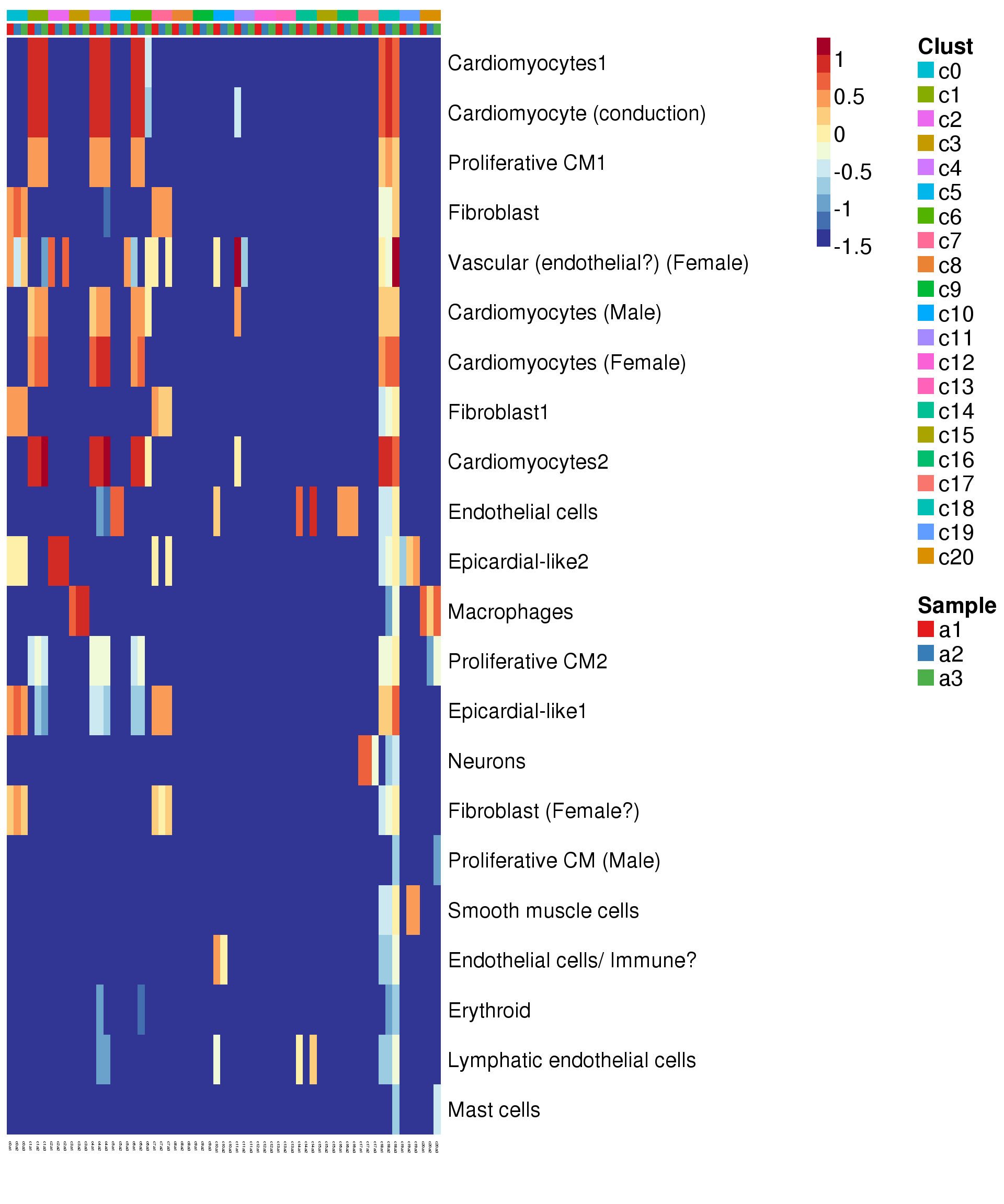
Compare adult to young
# This loads a list object called young.sig.genes.gst
load(file="./data/gstlist-young.Rdata")
expr.score <- matrix(NA,nrow=length(young.sig.genes.gst),ncol=length(levels(newgrp)))
colnames(expr.score) <- levels(newgrp)
rownames(expr.score) <- names(young.sig.genes.gst)
specialm <- lapply(young.sig.genes.gst,function(x) match(x,rownames(sumexpr))[!is.na(match(x,rownames(sumexpr)))])
for(i in 1:nrow(expr.score)){
expr.score[i,] <- colMedians(sumexpr[specialm[[i]],])
}
pdf(file="./output/Figures/heatmap-match-young-adult-medians.pdf",width=20,height=15,onefile = FALSE)
aheatmap(expr.score,
         Rowv = NA,Colv = NA,
         labRow = rownames(expr.score),
         annCol=list(Clust=clust,Sample=samps),
         annColors=myColors,
         fontsize=16,color="-RdYlBu",
         scale="none")
dev.off()png
2 aheatmap(expr.score,
Rowv = NA,Colv = NA,
labRow = rownames(expr.score),
annCol=list(Clust=clust,Sample=samps),
annColors=myColors,
fontsize=16,color="-RdYlBu",
scale="none")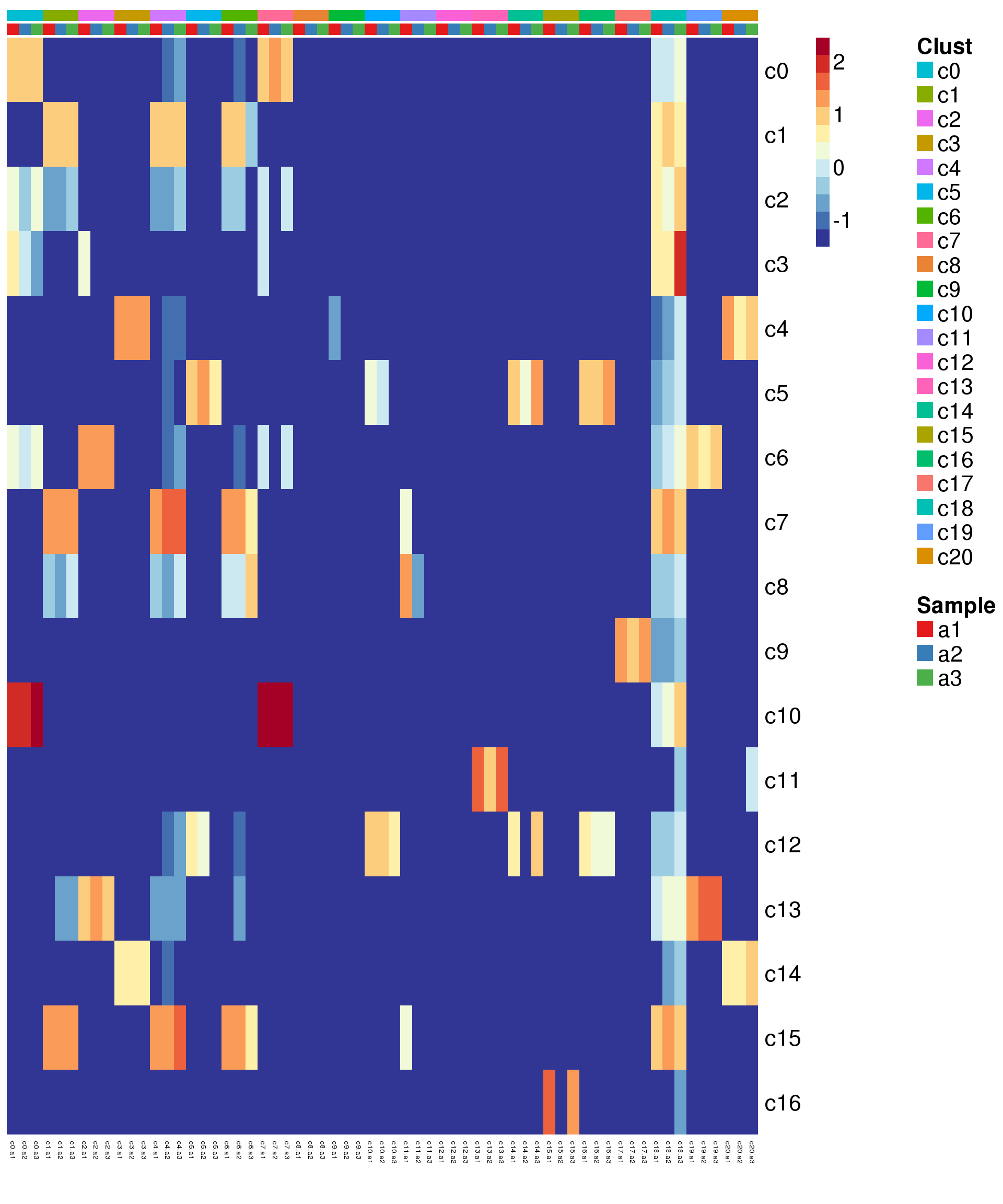
sessionInfo()R version 3.6.0 (2019-04-26)
Platform: x86_64-pc-linux-gnu (64-bit)
Running under: CentOS release 6.7 (Final)
Matrix products: default
BLAS: /usr/local/installed/R/3.6.0/lib64/R/lib/libRblas.so
LAPACK: /usr/local/installed/R/3.6.0/lib64/R/lib/libRlapack.so
locale:
[1] LC_CTYPE=en_US.UTF-8 LC_NUMERIC=C
[3] LC_TIME=en_US.UTF-8 LC_COLLATE=en_US.UTF-8
[5] LC_MONETARY=en_US.UTF-8 LC_MESSAGES=en_US.UTF-8
[7] LC_PAPER=en_US.UTF-8 LC_NAME=C
[9] LC_ADDRESS=C LC_TELEPHONE=C
[11] LC_MEASUREMENT=en_US.UTF-8 LC_IDENTIFICATION=C
attached base packages:
[1] splines parallel stats4 stats graphics grDevices utils
[8] datasets methods base
other attached packages:
[1] dplyr_0.8.1 clustree_0.4.0
[3] ggraph_1.0.2 workflowr_1.3.0
[5] NMF_0.21.0 bigmemory_4.5.33
[7] cluster_2.0.9 rngtools_1.3.1.1
[9] pkgmaker_0.27 registry_0.5-1
[11] scran_1.12.0 SingleCellExperiment_1.6.0
[13] SummarizedExperiment_1.14.0 GenomicRanges_1.36.0
[15] GenomeInfoDb_1.20.0 DelayedArray_0.10.0
[17] BiocParallel_1.18.0 matrixStats_0.54.0
[19] cowplot_0.9.4 monocle_2.12.0
[21] DDRTree_0.1.5 irlba_2.3.3
[23] VGAM_1.1-1 ggplot2_3.1.1
[25] Matrix_1.2-17 Seurat_3.0.2
[27] org.Hs.eg.db_3.8.2 AnnotationDbi_1.46.0
[29] IRanges_2.18.0 S4Vectors_0.22.0
[31] Biobase_2.44.0 BiocGenerics_0.30.0
[33] RColorBrewer_1.1-2 edgeR_3.26.3
[35] limma_3.40.2
loaded via a namespace (and not attached):
[1] reticulate_1.12 R.utils_2.8.0
[3] tidyselect_0.2.5 RSQLite_2.1.1
[5] htmlwidgets_1.3 grid_3.6.0
[7] combinat_0.0-8 docopt_0.6.1
[9] Rtsne_0.15 munsell_0.5.0
[11] codetools_0.2-16 ica_1.0-2
[13] statmod_1.4.30 future_1.12.0
[15] withr_2.1.2 colorspace_1.4-1
[17] fastICA_1.2-1 knitr_1.22
[19] ROCR_1.0-7 gbRd_0.4-11
[21] listenv_0.7.0 Rdpack_0.11-0
[23] labeling_0.3 git2r_0.25.2
[25] slam_0.1-45 GenomeInfoDbData_1.2.1
[27] polyclip_1.10-0 bit64_0.9-7
[29] farver_1.1.0 pheatmap_1.0.12
[31] rprojroot_1.3-2 xfun_0.6
[33] R6_2.4.0 doParallel_1.0.14
[35] ggbeeswarm_0.6.0 rsvd_1.0.0
[37] locfit_1.5-9.1 bitops_1.0-6
[39] assertthat_0.2.1 SDMTools_1.1-221.1
[41] scales_1.0.0 beeswarm_0.2.3
[43] gtable_0.3.0 npsurv_0.4-0
[45] globals_0.12.4 tidygraph_1.1.2
[47] rlang_0.3.4 lazyeval_0.2.2
[49] checkmate_1.9.3 yaml_2.2.0
[51] reshape2_1.4.3 backports_1.1.4
[53] tools_3.6.0 gridBase_0.4-7
[55] gplots_3.0.1.1 dynamicTreeCut_1.63-1
[57] ggridges_0.5.1 Rcpp_1.0.1
[59] plyr_1.8.4 zlibbioc_1.30.0
[61] purrr_0.3.2 RCurl_1.95-4.12
[63] densityClust_0.3 pbapply_1.4-0
[65] viridis_0.5.1 zoo_1.8-5
[67] ggrepel_0.8.1 fs_1.3.1
[69] magrittr_1.5 data.table_1.11.6
[71] lmtest_0.9-37 RANN_2.6.1
[73] whisker_0.3-2 fitdistrplus_1.0-14
[75] lsei_1.2-0 evaluate_0.13
[77] xtable_1.8-4 sparsesvd_0.1-4
[79] gridExtra_2.3 HSMMSingleCell_1.4.0
[81] compiler_3.6.0 scater_1.12.2
[83] tibble_2.1.1 KernSmooth_2.23-15
[85] crayon_1.3.4 R.oo_1.22.0
[87] htmltools_0.3.6 tidyr_0.8.3
[89] DBI_1.0.0 tweenr_1.0.1
[91] MASS_7.3-51.4 R.methodsS3_1.7.1
[93] gdata_2.18.0 metap_1.1
[95] igraph_1.2.4.1 pkgconfig_2.0.2
[97] bigmemory.sri_0.1.3 plotly_4.9.0
[99] foreach_1.4.4 vipor_0.4.5
[101] dqrng_0.2.1 XVector_0.24.0
[103] bibtex_0.4.2 stringr_1.4.0
[105] digest_0.6.18 sctransform_0.2.0
[107] tsne_0.1-3 rmarkdown_1.12.6
[109] DelayedMatrixStats_1.6.0 gtools_3.8.1
[111] nlme_3.1-139 jsonlite_1.6
[113] BiocNeighbors_1.2.0 viridisLite_0.3.0
[115] pillar_1.3.1 lattice_0.20-38
[117] GO.db_3.8.2 httr_1.4.0
[119] survival_2.44-1.1 glue_1.3.1
[121] qlcMatrix_0.9.7 FNN_1.1.3
[123] png_0.1-7 iterators_1.0.10
[125] bit_1.1-14 ggforce_0.2.2
[127] stringi_1.4.3 blob_1.1.1
[129] BiocSingular_1.0.0 caTools_1.17.1.2
[131] memoise_1.1.0 future.apply_1.2.0
[133] ape_5.3