apaQTLs
Briana Mittleman
4/18/2019
Last updated: 2019-04-29
Checks: 6 0
Knit directory: apaQTL/analysis/
This reproducible R Markdown analysis was created with workflowr (version 1.3.0). The Checks tab describes the reproducibility checks that were applied when the results were created. The Past versions tab lists the development history.
Great! Since the R Markdown file has been committed to the Git repository, you know the exact version of the code that produced these results.
Great job! The global environment was empty. Objects defined in the global environment can affect the analysis in your R Markdown file in unknown ways. For reproduciblity it’s best to always run the code in an empty environment.
The command set.seed(20190411) was run prior to running the code in the R Markdown file. Setting a seed ensures that any results that rely on randomness, e.g. subsampling or permutations, are reproducible.
Great job! Recording the operating system, R version, and package versions is critical for reproducibility.
Nice! There were no cached chunks for this analysis, so you can be confident that you successfully produced the results during this run.
Great! You are using Git for version control. Tracking code development and connecting the code version to the results is critical for reproducibility. The version displayed above was the version of the Git repository at the time these results were generated.
Note that you need to be careful to ensure that all relevant files for the analysis have been committed to Git prior to generating the results (you can use wflow_publish or wflow_git_commit). workflowr only checks the R Markdown file, but you know if there are other scripts or data files that it depends on. Below is the status of the Git repository when the results were generated:
Ignored files:
    Ignored:    .DS_Store
    Ignored:    .Rhistory
    Ignored:    .Rproj.user/
    Ignored:    output/.DS_Store

Untracked files:
    Untracked:  .Rprofile
    Untracked:  ._.DS_Store
    Untracked:  .gitignore
    Untracked:  _workflowr.yml
    Untracked:  analysis/._PASdescriptiveplots.Rmd
    Untracked:  analysis/._cuttoffPercUsage.Rmd
    Untracked:  analysis/cuttoffPercUsage.Rmd
    Untracked:  analysis/newQTLheatmap.Rmd
    Untracked:  apaQTL.Rproj
    Untracked:  code/._SnakefilePAS
    Untracked:  code/._SnakefilefiltPAS
    Untracked:  code/._apaQTLCorrectPvalMakeQQ.R
    Untracked:  code/._apaQTL_Nominal.sh
    Untracked:  code/._apaQTL_permuted.sh
    Untracked:  code/._bed2saf.py
    Untracked:  code/._callPeaksYL.py
    Untracked:  code/._chooseAnno2SAF.py
    Untracked:  code/._chooseSignalSite
    Untracked:  code/._chooseSignalSite.py
    Untracked:  code/._cluster.json
    Untracked:  code/._clusterPAS.json
    Untracked:  code/._clusterfiltPAS.json
    Untracked:  code/._config.yaml
    Untracked:  code/._config2.yaml
    Untracked:  code/._configOLD.yaml
    Untracked:  code/._convertNumeric.py
    Untracked:  code/._dag.pdf
    Untracked:  code/._filter5perc.R
    Untracked:  code/._filter5percPheno.py
    Untracked:  code/._filterpeaks.py
    Untracked:  code/._fixFChead.py
    Untracked:  code/._make5percPeakbed.py
    Untracked:  code/._makeFileID.py
    Untracked:  code/._makePheno.py
    Untracked:  code/._mergeAllBam.sh
    Untracked:  code/._mergeByFracBam.sh
    Untracked:  code/._mergePeaks.sh
    Untracked:  code/._namePeaks.py
    Untracked:  code/._peak2PAS.py
    Untracked:  code/._peakFC.sh
    Untracked:  code/._pheno2countonly.R
    Untracked:  code/._quantassign2parsedpeak.py
    Untracked:  code/._snakemakePAS.batch
    Untracked:  code/._snakemakefiltPAS.batch
    Untracked:  code/._submit-snakemakePAS.sh
    Untracked:  code/._submit-snakemakefiltPAS.sh
    Untracked:  code/.snakemake/
    Untracked:  code/APAqtl_nominal.err
    Untracked:  code/APAqtl_nominal.out
    Untracked:  code/APAqtl_permuted.err
    Untracked:  code/APAqtl_permuted.out
    Untracked:  code/BothFracDTPlotGeneRegions.err
    Untracked:  code/BothFracDTPlotGeneRegions.out
    Untracked:  code/DistPAS2Sig.py
    Untracked:  code/README.md
    Untracked:  code/Rplots.pdf
    Untracked:  code/Upstream100Bases_general.py
    Untracked:  code/bam2bw.err
    Untracked:  code/bam2bw.out
    Untracked:  code/dag.pdf
    Untracked:  code/dagPAS.pdf
    Untracked:  code/dagfiltPAS.pdf
    Untracked:  code/findbuginpeaks.R
    Untracked:  code/get100upPAS.py
    Untracked:  code/getSeq100up.sh
    Untracked:  code/getseq100up.err
    Untracked:  code/getseq100up.out
    Untracked:  code/log/
    Untracked:  code/run_DistPAS2Sig.err
    Untracked:  code/run_DistPAS2Sig.out
    Untracked:  code/run_distPAS2Sig.sh
    Untracked:  code/snakePASlog.out
    Untracked:  code/snakefiltPASlog.out
    Untracked:  data/DTmatrix/
    Untracked:  data/PAS/
    Untracked:  data/README.md
    Untracked:  data/SignalSiteFiles/
    Untracked:  data/apaQTLNominal/
    Untracked:  data/apaQTLPermuted/
    Untracked:  data/apaQTLs/
    Untracked:  data/assignedPeaks/
    Untracked:  data/bam/
    Untracked:  data/bam_clean/
    Untracked:  data/bam_waspfilt/
    Untracked:  data/bed_10up/
    Untracked:  data/bed_clean/
    Untracked:  data/bed_clean_sort/
    Untracked:  data/bed_waspfilter/
    Untracked:  data/bedsort_waspfilter/
    Untracked:  data/fastq/
    Untracked:  data/filterPeaks/
    Untracked:  data/inclusivePeaks/
    Untracked:  data/inclusivePeaks_FC/
    Untracked:  data/mergedBG/
    Untracked:  data/mergedBW_byfrac/
    Untracked:  data/mergedBam/
    Untracked:  data/mergedbyFracBam/
    Untracked:  data/nuc_10up/
    Untracked:  data/nuc_10upclean/
    Untracked:  data/peakCoverage/
    Untracked:  data/peaks_5perc/
    Untracked:  data/phenotype/
    Untracked:  data/phenotype_5perc/
    Untracked:  data/sort/
    Untracked:  data/sort_clean/
    Untracked:  data/sort_waspfilter/
    Untracked:  nohup.out
    Untracked:  output/._.DS_Store
    Untracked:  output/dtPlots/
    Untracked:  output/fastqc/

Unstaged changes:
    Modified:   analysis/PASusageQC.Rmd
    Modified:   analysis/corrbetweenind.Rmd
    Deleted:    code/Upstream10Bases_general.py
    Modified:   code/apaQTLCorrectPvalMakeQQ.R
    Modified:   code/apaQTL_permuted.sh
    Modified:   code/bed2saf.py
    Deleted:    code/test.txt
Note that any generated files, e.g. HTML, png, CSS, etc., are not included in this status report because it is ok for generated content to have uncommitted changes.
These are the previous versions of the R Markdown and HTML files. If you’ve configured a remote Git repository (see ?wflow_git_remote), click on the hyperlinks in the table below to view them.
| File | Version | Author | Date | Message |
|---|---|---|---|---|
| Rmd | 3c5e041 | brimittleman | 2019-04-29 | add write out for qtls |
| html | 9490b23 | brimittleman | 2019-04-29 | Build site. |
| Rmd | b18b96c | brimittleman | 2019-04-29 | fix distance |
| html | 2d33728 | brimittleman | 2019-04-28 | Build site. |
| Rmd | 7416404 | brimittleman | 2019-04-28 | add res |
| html | ed97e35 | brimittleman | 2019-04-21 | Build site. |
| Rmd | be90ded | brimittleman | 2019-04-21 | fix to 5perc phenp |
| html | 28bd046 | brimittleman | 2019-04-18 | Build site. |
| Rmd | 017f5c0 | brimittleman | 2019-04-18 | add map apa qtl pipeline |
library(tidyverse)── Attaching packages ─────────────────────────────────────────────── tidyverse 1.2.1 ──✔ ggplot2 3.1.0 ✔ purrr 0.3.2
✔ tibble 2.1.1 ✔ dplyr 0.8.0.1
✔ tidyr 0.8.3 ✔ stringr 1.3.1
✔ readr 1.3.1 ✔ forcats 0.3.0 ── Conflicts ────────────────────────────────────────────────── tidyverse_conflicts() ──
✖ dplyr::filter() masks stats::filter()
✖ dplyr::lag() masks stats::lag()library(reshape2)
Attaching package: 'reshape2'The following object is masked from 'package:tidyr':
smithslibrary(workflowr)This is workflowr version 1.3.0
Run ?workflowr for help getting startedlibrary(cowplot)
Attaching package: 'cowplot'The following object is masked from 'package:ggplot2':
ggsaveIn this analysis I will call apaQTls in both fractions. I will start with the phenotype files and normalized the counts using the leafcutter package in order to run the fastq QTL mapper.
Prepare phenotypes for QTL- phenotype dir
It is best to run this analysis in the data/phenotype_5perc directory. I have copied the leafcutter prepare_phenotype_table.py to the code directroy to use here.
#!/bin/bash
module load python

gzip APApeak_Phenotype_GeneLocAnno.Total.5perc.fc
gzip APApeak_Phenotype_GeneLocAnno.Nuclear.5perc.fc

python ../../code/prepare_phenotype_table.py APApeak_Phenotype_GeneLocAnno.Total.5perc.fc.gz
python ../../code/prepare_phenotype_table.py APApeak_Phenotype_GeneLocAnno.Nuclear.5perc.fc.gz
This will output bash scripts to run.
module load Anaconda3
source activate three-prime-env

sh APApeak_Phenotype_GeneLocAnno.Nuclear.5perc.fc.gz_prepare.sh
sh APApeak_Phenotype_GeneLocAnno.Total.5perc.fc.gz_prepare.sh
Subset the PCs to use the first 2 in the qtl calling:
module load Anaconda3
source activate three-prime-env

head -n 3 APApeak_Phenotype_GeneLocAnno.Nuclear.5perc.fc.gz.PCs > APApeak_Phenotype_GeneLocAnno.Nuclear.5perc.fc.gz.2PCs
head -n 3 APApeak_Phenotype_GeneLocAnno.Total.5perc.fc.gz.PCs > APApeak_Phenotype_GeneLocAnno.Total.5perc.fc.gz.2PCs
Call QTLs- code dir
Next I will need to make a sample list. From the code directory:
python makeSampleList.pyremove 19092 and 19193
Prepare directroy
mkdir ../data/apaQTLNominal
mkdir ../data/apaQTLPermuted
Run the code to call QTLs within 1mb of each PAS peak. I run both a nominal pass and a permuted pas. The permulted pas chosses the best snp for each peak gene pair.
sbatch apaQTL_Nominal.sh
sbatch apaQTL_permuted.sh
Concatinate all of the results in the permuted set. I do this so I can account for multiple testing with the benjamini hochberg test.
Concatinate results in permuted directory:
cat APApeak_Phenotype_GeneLocAnno.Total.5perc.fc.gz.qqnorm_chr* > APApeak_Phenotype_GeneLocAnno.Total_permRes.txt

cat APApeak_Phenotype_GeneLocAnno.Nuclear.5perc.fc.gz.qqnorm_chr* > APApeak_Phenotype_GeneLocAnno.Nuclear_permRes.txt
Run correction script
Rscripts apaQTLCorrectPvalMakeQQ.R Evaluation results
totRes=read.table("../data/apaQTLPermuted/APApeak_Phenotype_GeneLocAnno.Total_permResBH.txt", stringsAsFactors = F, header = T) %>% separate(pid, into=c("Chr", "Start", "End", "PeakID"), sep=":") %>% separate(PeakID, into=c("Gene", "Loc", "Strand","Peak"), sep="_")Total Apa QTLs
TotQTLs= totRes %>% filter(-log10(bh)>=1)
nrow(TotQTLs)
[1] 502apaQTL genes:
TotQTLs_gene=TotQTLs %>% group_by(Gene)  %>% summarise(nQTL=n())

summary(TotQTLs_gene$nQTL)
Min. 1st Qu. Median Mean 3rd Qu. Max.
1.000 1.000 1.000 1.307 2.000 6.000 hist(TotQTLs_gene$nQTL)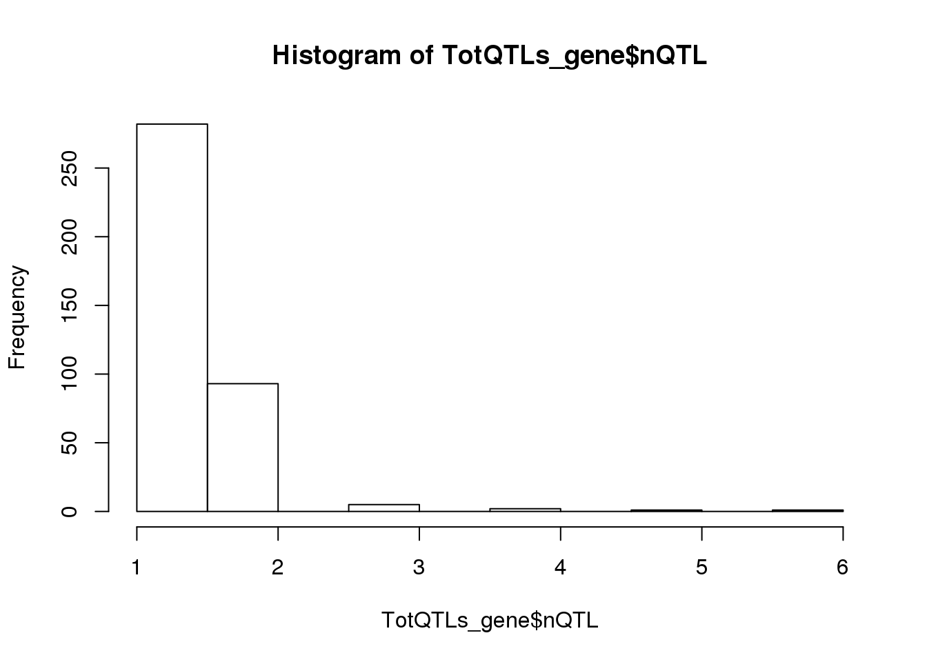
Location distribution for peaks:
TotQTLs_loc= TotQTLs %>% group_by(Loc) %>% summarise(nLoc=n()) %>% mutate(PropLoc=nLoc/nrow(TotQTLs))


totQTLloc=ggplot(TotQTLs_loc, aes(x=Loc, y=PropLoc, fill=Loc)) + geom_bar(stat = "Identity") + labs(x="Location of Significant Peak", y="Proportion of QTLs", title="Total QTL peak distribution")+ theme(axis.text.x = element_text(angle = 90, hjust = 1))
nucRes=read.table("../data/apaQTLPermuted/APApeak_Phenotype_GeneLocAnno.Nuclear_permResBH.txt", stringsAsFactors = F, header = T) %>% separate(pid, into=c("Chr", "Start", "End", "PeakID"), sep=":") %>% separate(PeakID, into=c("Gene", "Loc", "Strand","Peak"), sep="_")Nuclear Apa QTLs
NucQTLs= nucRes %>% filter(-log10(bh)>=1)
nrow(NucQTLs)
[1] 1070apaQTL genes:
NucQTLs_gene= NucQTLs %>% group_by(Gene)  %>% summarise(nQTL=n())

summary(NucQTLs_gene$nQTL)
Min. 1st Qu. Median Mean 3rd Qu. Max.
1.000 1.000 1.000 1.328 2.000 7.000 hist(NucQTLs_gene$nQTL)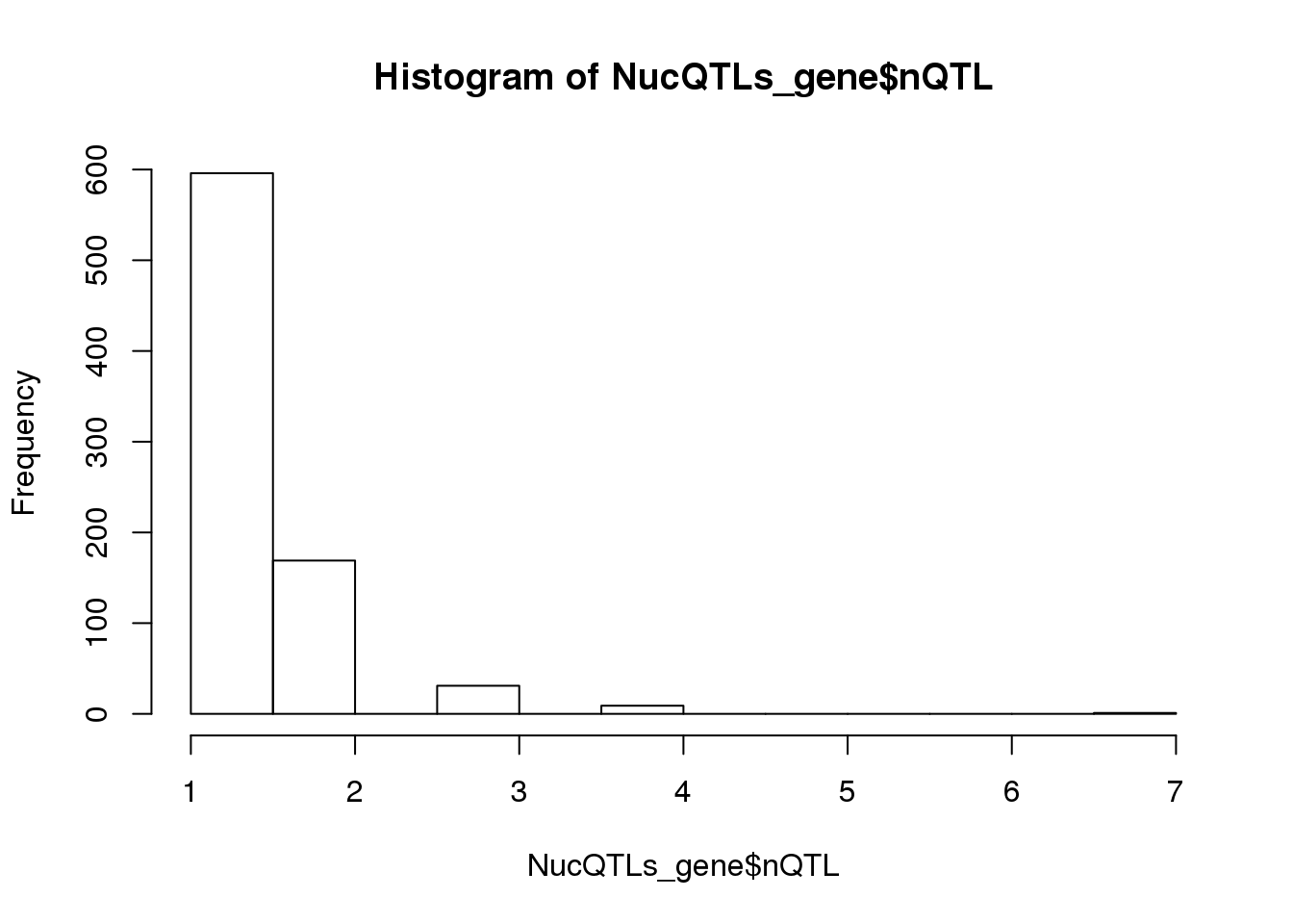
Location distribution for peaks:
NucQTLs_loc= NucQTLs %>% group_by(Loc) %>% summarise(nLoc=n()) %>% mutate(PropLoc=nLoc/nrow(NucQTLs))


nucQTLloc=ggplot(NucQTLs_loc, aes(x=Loc, y=PropLoc, fill=Loc)) + geom_bar(stat = "Identity") + labs(x="Location of Significant Peak", y="Proportion of QTLs", title="Nuclear QTL peak distribution")+theme(axis.text.x = element_text(angle = 90, hjust = 1))
plot_grid(totQTLloc, nucQTLloc)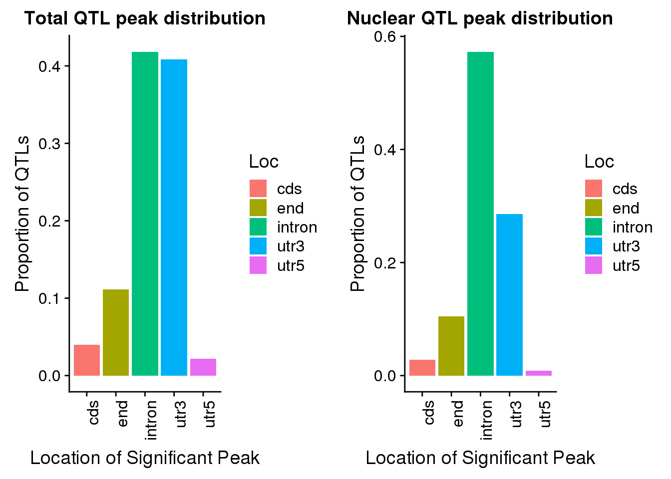
Distance to PAS
The distance to PAS is the location of the snp to the end of the peak for the
Strand in this file is the peak strand (opposite of gene). This means for + strand I want the start of the Peak and for the - strand i will use the end of the peak. ###Total
TotQTLs_dist=TotQTLs %>% separate(sid, into=c("SnpCHR", "SNPpos"), sep=":") %>% mutate(Dist2PAS=ifelse(Strand=="+", as.integer(SNPpos)-as.integer(Start), as.integer(SNPpos)-as.integer(End)))


summary(abs(TotQTLs_dist$Dist2PAS))
Min. 1st Qu. Median Mean 3rd Qu. Max.
0 1598 6160 8832 15461 25071 Plot:
totqtldist=ggplot(TotQTLs_dist, aes(x=Dist2PAS)) + geom_histogram(bins=100, fill="darkviolet") + theme(axis.text.x = element_text(angle = 90, hjust = 1)) + labs(x="Distance from QTL snp to PAS",y="Number of Total apaQTLs", title="Total apaQTL \n are close to the PAS they regulate")ggplot(TotQTLs_dist, aes(x=Dist2PAS)) + geom_histogram(bins=100) + theme(axis.text.x = element_text(angle = 90, hjust = 1)) + facet_grid(~Loc)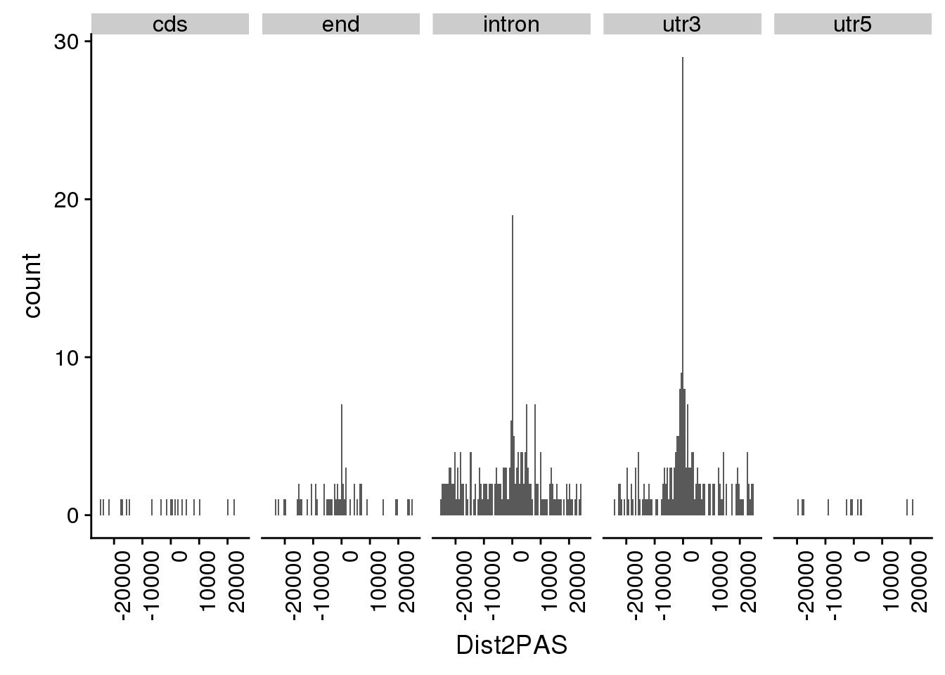
| Version | Author | Date |
|---|---|---|
| 9490b23 | brimittleman | 2019-04-29 |
Nuclear
NucQTLs_dist=NucQTLs %>% separate(sid, into=c("SnpCHR", "SNPpos"), sep=":") %>% mutate(Dist2PAS=ifelse(Strand=="+", as.integer(SNPpos)-as.integer(Start), as.integer(SNPpos)-as.integer(End)))


summary(abs(NucQTLs_dist$Dist2PAS))
Min. 1st Qu. Median Mean 3rd Qu. Max.
0 1930 7726 9216 15463 25071 Plot:
nucqtldist=ggplot(NucQTLs_dist, aes(x=Dist2PAS)) + geom_histogram(bins=100,fill="deepskyblue3") + theme(axis.text.x = element_text(angle = 90, hjust = 1)) + labs(x="Distance from QTL snp to PAS",y="Number of Nuclear apaQTLs", title="Nuclear apaQTL \n are close to the PAS they regulate") plot_grid(totqtldist,nucqtldist)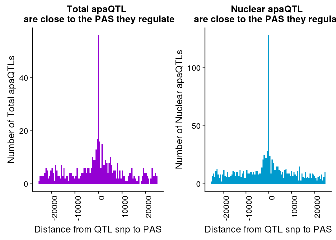
Write out QTLs:
write.table(TotQTLs, file="../data/apaQTLs/Total_apaQTLs_5fdr.txt", col.names = T, row.names = F, quote=F)

write.table(NucQTLs, file="../data/apaQTLs/Nuclear_apaQTLs_5fdr.txt", col.names = T, row.names = F, quote=F)
sessionInfo()R version 3.5.1 (2018-07-02)
Platform: x86_64-pc-linux-gnu (64-bit)
Running under: Scientific Linux 7.4 (Nitrogen)
Matrix products: default
BLAS/LAPACK: /software/openblas-0.2.19-el7-x86_64/lib/libopenblas_haswellp-r0.2.19.so
locale:
[1] LC_CTYPE=en_US.UTF-8 LC_NUMERIC=C
[3] LC_TIME=en_US.UTF-8 LC_COLLATE=en_US.UTF-8
[5] LC_MONETARY=en_US.UTF-8 LC_MESSAGES=en_US.UTF-8
[7] LC_PAPER=en_US.UTF-8 LC_NAME=C
[9] LC_ADDRESS=C LC_TELEPHONE=C
[11] LC_MEASUREMENT=en_US.UTF-8 LC_IDENTIFICATION=C
attached base packages:
[1] stats graphics grDevices utils datasets methods base
other attached packages:
[1] cowplot_0.9.4 workflowr_1.3.0 reshape2_1.4.3 forcats_0.3.0
[5] stringr_1.3.1 dplyr_0.8.0.1 purrr_0.3.2 readr_1.3.1
[9] tidyr_0.8.3 tibble_2.1.1 ggplot2_3.1.0 tidyverse_1.2.1
loaded via a namespace (and not attached):
[1] Rcpp_1.0.0 cellranger_1.1.0 pillar_1.3.1 compiler_3.5.1
[5] git2r_0.23.0 plyr_1.8.4 tools_3.5.1 digest_0.6.18
[9] lubridate_1.7.4 jsonlite_1.6 evaluate_0.12 nlme_3.1-137
[13] gtable_0.2.0 lattice_0.20-38 pkgconfig_2.0.2 rlang_0.3.1
[17] cli_1.0.1 rstudioapi_0.10 yaml_2.2.0 haven_1.1.2
[21] withr_2.1.2 xml2_1.2.0 httr_1.3.1 knitr_1.20
[25] hms_0.4.2 generics_0.0.2 fs_1.2.6 rprojroot_1.3-2
[29] grid_3.5.1 tidyselect_0.2.5 glue_1.3.0 R6_2.3.0
[33] readxl_1.1.0 rmarkdown_1.10 modelr_0.1.2 magrittr_1.5
[37] whisker_0.3-2 backports_1.1.2 scales_1.0.0 htmltools_0.3.6
[41] rvest_0.3.2 assertthat_0.2.0 colorspace_1.3-2 labeling_0.3
[45] stringi_1.2.4 lazyeval_0.2.1 munsell_0.5.0 broom_0.5.1
[49] crayon_1.3.4