Characterize Nuclear ApaQTLs
Briana Mittleman
10/24/2018
Last updated: 2018-10-29
workflowr checks: (Click a bullet for more information)-
✔ R Markdown file: up-to-date
Great! Since the R Markdown file has been committed to the Git repository, you know the exact version of the code that produced these results.
-
✔ Environment: empty
Great job! The global environment was empty. Objects defined in the global environment can affect the analysis in your R Markdown file in unknown ways. For reproduciblity it’s best to always run the code in an empty environment.
-
✔ Seed:
set.seed(12345)The command
set.seed(12345)was run prior to running the code in the R Markdown file. Setting a seed ensures that any results that rely on randomness, e.g. subsampling or permutations, are reproducible. -
✔ Session information: recorded
Great job! Recording the operating system, R version, and package versions is critical for reproducibility.
-
Great! You are using Git for version control. Tracking code development and connecting the code version to the results is critical for reproducibility. The version displayed above was the version of the Git repository at the time these results were generated.✔ Repository version: afb0ce9
Note that you need to be careful to ensure that all relevant files for the analysis have been committed to Git prior to generating the results (you can usewflow_publishorwflow_git_commit). workflowr only checks the R Markdown file, but you know if there are other scripts or data files that it depends on. Below is the status of the Git repository when the results were generated:
Note that any generated files, e.g. HTML, png, CSS, etc., are not included in this status report because it is ok for generated content to have uncommitted changes.Ignored files: Ignored: .DS_Store Ignored: .Rhistory Ignored: .Rproj.user/ Ignored: data/.DS_Store Ignored: output/.DS_Store Untracked files: Untracked: KalistoAbundance18486.txt Untracked: analysis/genometrack_figs.Rmd Untracked: analysis/ncbiRefSeq_sm.sort.mRNA.bed Untracked: analysis/snake.config.notes.Rmd Untracked: analysis/verifyBAM.Rmd Untracked: data/18486.genecov.txt Untracked: data/APApeaksYL.total.inbrain.bed Untracked: data/ChromHmmOverlap/ Untracked: data/GM12878.chromHMM.bed Untracked: data/GM12878.chromHMM.txt Untracked: data/NuclearApaQTLs.txt Untracked: data/PeaksUsed/ Untracked: data/RNAkalisto/ Untracked: data/TotalApaQTLs.txt Untracked: data/Totalpeaks_filtered_clean.bed Untracked: data/YL-SP-18486-T-combined-genecov.txt Untracked: data/YL-SP-18486-T_S9_R1_001-genecov.txt Untracked: data/apaExamp/ Untracked: data/bedgraph_peaks/ Untracked: data/bin200.5.T.nuccov.bed Untracked: data/bin200.Anuccov.bed Untracked: data/bin200.nuccov.bed Untracked: data/clean_peaks/ Untracked: data/comb_map_stats.csv Untracked: data/comb_map_stats.xlsx Untracked: data/comb_map_stats_39ind.csv Untracked: data/combined_reads_mapped_three_prime_seq.csv Untracked: data/diff_iso_trans/ Untracked: data/ensemble_to_genename.txt Untracked: data/filtered_APApeaks_merged_allchrom_refseqTrans.closest2End.bed Untracked: data/filtered_APApeaks_merged_allchrom_refseqTrans.closest2End.noties.bed Untracked: data/first50lines_closest.txt Untracked: data/gencov.test.csv Untracked: data/gencov.test.txt Untracked: data/gencov_zero.test.csv Untracked: data/gencov_zero.test.txt Untracked: data/gene_cov/ Untracked: data/joined Untracked: data/leafcutter/ Untracked: data/merged_combined_YL-SP-threeprimeseq.bg Untracked: data/mol_overlap/ Untracked: data/mol_pheno/ Untracked: data/nom_QTL/ Untracked: data/nom_QTL_opp/ Untracked: data/nom_QTL_trans/ Untracked: data/nuc6up/ Untracked: data/other_qtls/ Untracked: data/peakPerRefSeqGene/ Untracked: data/perm_QTL/ Untracked: data/perm_QTL_opp/ Untracked: data/perm_QTL_trans/ Untracked: data/reads_mapped_three_prime_seq.csv Untracked: data/smash.cov.results.bed Untracked: data/smash.cov.results.csv Untracked: data/smash.cov.results.txt Untracked: data/smash_testregion/ Untracked: data/ssFC200.cov.bed Untracked: data/temp.file1 Untracked: data/temp.file2 Untracked: data/temp.gencov.test.txt Untracked: data/temp.gencov_zero.test.txt Untracked: output/picard/ Untracked: output/plots/ Untracked: output/qual.fig2.pdf Unstaged changes: Modified: analysis/28ind.peak.explore.Rmd Modified: analysis/39indQC.Rmd Modified: analysis/cleanupdtseq.internalpriming.Rmd Modified: analysis/coloc_apaQTLs_protQTLs.Rmd Modified: analysis/dif.iso.usage.leafcutter.Rmd Modified: analysis/diff_iso_pipeline.Rmd Modified: analysis/explore.filters.Rmd Modified: analysis/overlapMolQTL.Rmd Modified: analysis/overlap_qtls.Rmd Modified: analysis/peakOverlap_oppstrand.Rmd Modified: analysis/pheno.leaf.comb.Rmd Modified: analysis/test.max2.Rmd Modified: code/Snakefile
Expand here to see past versions:
| File | Version | Author | Date | Message |
|---|---|---|---|---|
| Rmd | afb0ce9 | Briana Mittleman | 2018-10-29 | change plot colors |
| html | 805dec6 | Briana Mittleman | 2018-10-26 | Build site. |
| Rmd | 5cb6b0b | Briana Mittleman | 2018-10-26 | permutation code |
| html | 96cfdcd | Briana Mittleman | 2018-10-24 | Build site. |
| Rmd | 00b1020 | Briana Mittleman | 2018-10-24 | naive enrichment |
| html | de860f0 | Briana Mittleman | 2018-10-24 | Build site. |
| Rmd | 96a97f4 | Briana Mittleman | 2018-10-24 | add nuclear characterization |
This analysis is similar to the Characterize Total APAqtl analysis
I would like to study:
- Distance metrics:
- distance from snp to TSS of gene
- Distance from snp to peak
- distance from snp to TSS of gene
- Expression metrics:
- expression of genes with significant QTLs vs other genes (by rna seq)
- expression of genes with significant QTLs vs other genes (peak coverage)
- Chrom HMM metrics:
- look at the chrom HMM interval for the significant QTLs
Upload Libraries and Data:
Library
library(workflowr)This is workflowr version 1.1.1
Run ?workflowr for help getting startedlibrary(reshape2)
library(tidyverse)── Attaching packages ──────────────────────────────────────────────────────────── tidyverse 1.2.1 ──✔ ggplot2 3.0.0 ✔ purrr 0.2.5
✔ tibble 1.4.2 ✔ dplyr 0.7.6
✔ tidyr 0.8.1 ✔ stringr 1.3.1
✔ readr 1.1.1 ✔ forcats 0.3.0── Conflicts ─────────────────────────────────────────────────────────────── tidyverse_conflicts() ──
✖ dplyr::filter() masks stats::filter()
✖ dplyr::lag() masks stats::lag()library(VennDiagram)Loading required package: gridLoading required package: futile.loggerlibrary(data.table)
Attaching package: 'data.table'The following objects are masked from 'package:dplyr':
between, first, lastThe following object is masked from 'package:purrr':
transposeThe following objects are masked from 'package:reshape2':
dcast, meltlibrary(cowplot)
Attaching package: 'cowplot'The following object is masked from 'package:ggplot2':
ggsavePermuted Results from APA:
I will add a column to this dataframe that will tell me if the association is significant at 10% FDR. This will help me plot based on significance later in the analysis. I am also going to seperate the PID into relevant pieces.
NuclearAPA=read.table("../data/perm_QTL_trans/filtered_APApeaks_merged_allchrom_refseqGenes_pheno_Nuclear_transcript_permResBH.txt", stringsAsFactors = F, header=T)  %>% mutate(sig=ifelse(-log10(bh)>=1, 1,0 )) %>%  separate(pid, sep = ":", into=c("chr", "start", "end", "id")) %>% separate(id, sep = "_", into=c("gene", "strand", "peak"))

NuclearAPA$sig=as.factor(NuclearAPA$sig)


print(names(NuclearAPA))
[1] "chr" "start" "end" "gene" "strand" "peak" "nvar"
[8] "shape1" "shape2" "dummy" "sid" "dist" "npval" "slope"
[15] "ppval" "bpval" "bh" "sig" Distance Metrics
Distance from snp to TSS
I ran the QTL analysis based on the starting position of the gene.
ggplot(NuclearAPA, aes(x=dist, fill=sig, by=sig)) + geom_density(alpha=.5) + labs(title="Distance from snp to TSS", x="Base Pairs") + scale_fill_discrete(guide = guide_legend(title = "Significant QTL")) + scale_fill_brewer(palette="Paired")Scale for 'fill' is already present. Adding another scale for 'fill',
which will replace the existing scale.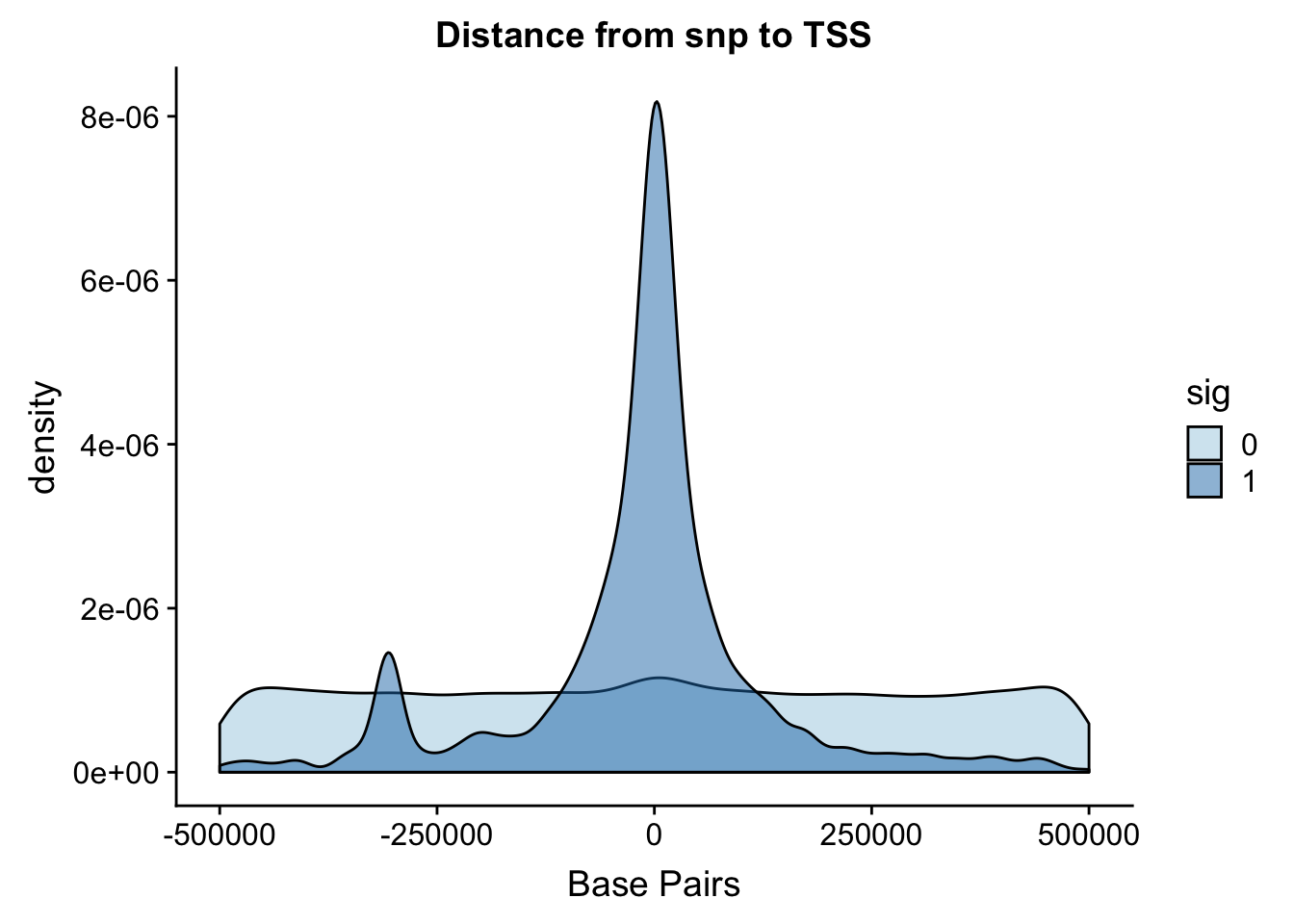
Expand here to see past versions of unnamed-chunk-3-1.png:
| Version | Author | Date |
|---|---|---|
| de860f0 | Briana Mittleman | 2018-10-24 |
Zoom in to 100,000.
ggplot(NuclearAPA, aes(x=dist, fill=sig, by=sig)) + geom_density(alpha=.5)+coord_cartesian(xlim = c(-150000, 150000)) + scale_fill_brewer(palette="Paired")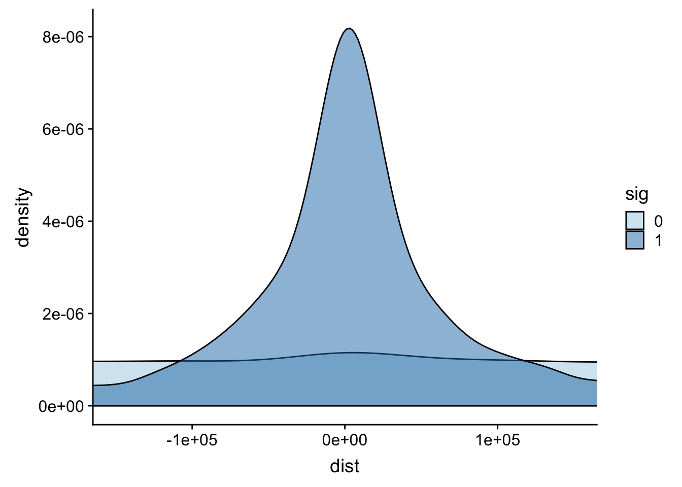
Expand here to see past versions of unnamed-chunk-4-1.png:
| Version | Author | Date |
|---|---|---|
| de860f0 | Briana Mittleman | 2018-10-24 |
Distance from snp to peak
To perform this analysis I need to recover the peak positions.
The peak file I used for the QTL analysis is: /project2/gilad/briana/threeprimeseq/data/mergedPeaks_comb/filtered_APApeaks_merged_allchrom_refseqTrans.noties_sm.fixed.bed
peaks=read.table("../data/PeaksUsed/filtered_APApeaks_merged_allchrom_refseqTrans.noties_sm.fixed.bed", col.names = c("chr", "peakStart", "peakEnd", "PeakNum", "PeakScore", "Strand", "Gene")) %>% mutate(peak=paste("peak", PeakNum,sep="")) %>% mutate(PeakCenter=peakStart+ (peakEnd- peakStart))I want to join the peak start to the NuclearAPA file but the peak column. I will then create a column that is snppos-peakcenter.
NuclearAPA_peakdist= NuclearAPA %>%  inner_join(peaks, by="peak") %>%  separate(sid, into=c("snpCHR", "snpLOC"), by=":")
NuclearAPA_peakdist$snpLOC= as.numeric(NuclearAPA_peakdist$snpLOC)

NuclearAPA_peakdist= NuclearAPA_peakdist %>%  mutate(DisttoPeak= snpLOC-PeakCenter)
Plot this by significance.
ggplot(NuclearAPA_peakdist, aes(x=DisttoPeak, fill=sig, by=sig)) + geom_density(alpha=.5) + labs(title="Distance from snp peak", x="log10 absolute value Distance to Peak") + scale_fill_discrete(guide = guide_legend(title = "Significant QTL")) + scale_fill_brewer(palette="Paired")Scale for 'fill' is already present. Adding another scale for 'fill',
which will replace the existing scale.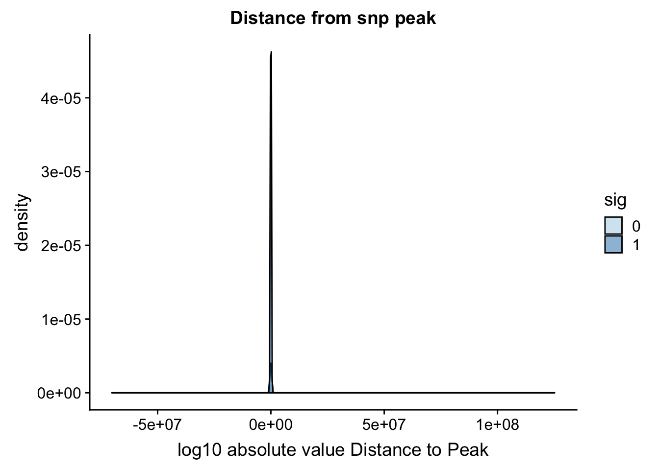
Expand here to see past versions of unnamed-chunk-7-1.png:
| Version | Author | Date |
|---|---|---|
| de860f0 | Briana Mittleman | 2018-10-24 |
Look at the summarys based on significance:
NuclearAPA_peakdist_sig=NuclearAPA_peakdist %>% filter(sig==1)
NuclearAPA_peakdist_notsig=NuclearAPA_peakdist %>% filter(sig==0)


summary(NuclearAPA_peakdist_sig$DisttoPeak)
Min. 1st Qu. Median Mean 3rd Qu. Max.
-1003786 -17579 -91 -8818 6588 891734 summary(NuclearAPA_peakdist_notsig$DisttoPeak) Min. 1st Qu. Median Mean 3rd Qu. Max.
-70147526 -265059 -2067 7263 255169 125172864 ggplot(NuclearAPA_peakdist, aes(y=DisttoPeak,x=sig, fill=sig, by=sig)) + geom_boxplot() + scale_fill_discrete(guide = guide_legend(title = "Significant QTL")) + scale_fill_brewer(palette="Paired")Scale for 'fill' is already present. Adding another scale for 'fill',
which will replace the existing scale.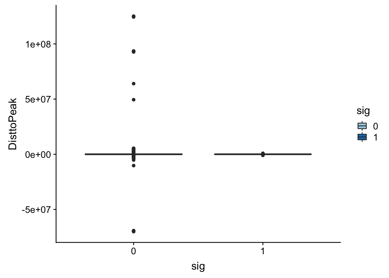
Expand here to see past versions of unnamed-chunk-9-1.png:
| Version | Author | Date |
|---|---|---|
| de860f0 | Briana Mittleman | 2018-10-24 |
Look like there are some outliers that are really far. I will remove variants greater than 1*10^6th away
NuclearAPA_peakdist_filt=NuclearAPA_peakdist %>% filter(abs(DisttoPeak) <= 1*(10^6))

ggplot(NuclearAPA_peakdist_filt, aes(y=DisttoPeak,x=sig, fill=sig, by=sig)) + geom_boxplot()  + scale_fill_discrete(guide = guide_legend(title = "Significant QTL")) + facet_grid(.~strand) + scale_fill_brewer(palette="Paired")
Scale for 'fill' is already present. Adding another scale for 'fill',
which will replace the existing scale.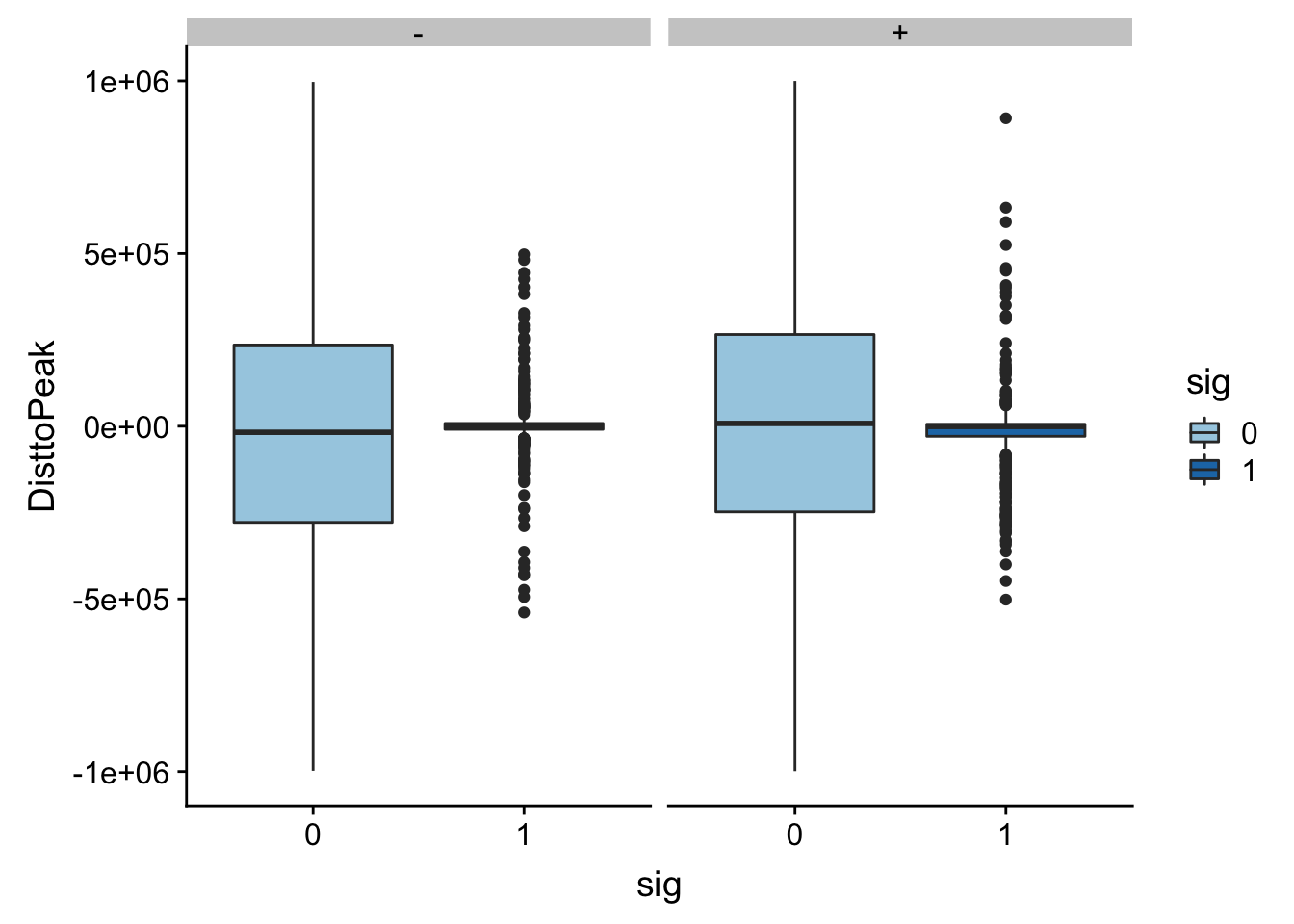
Expand here to see past versions of unnamed-chunk-10-1.png:
| Version | Author | Date |
|---|---|---|
| de860f0 | Briana Mittleman | 2018-10-24 |
ggplot(NuclearAPA_peakdist_filt, aes(x=DisttoPeak, fill=sig, by=sig)) + geom_density() + scale_fill_discrete(guide = guide_legend(title = "Significant QTL")) + facet_grid(.~strand)+ scale_fill_brewer(palette="Paired")Scale for 'fill' is already present. Adding another scale for 'fill',
which will replace the existing scale.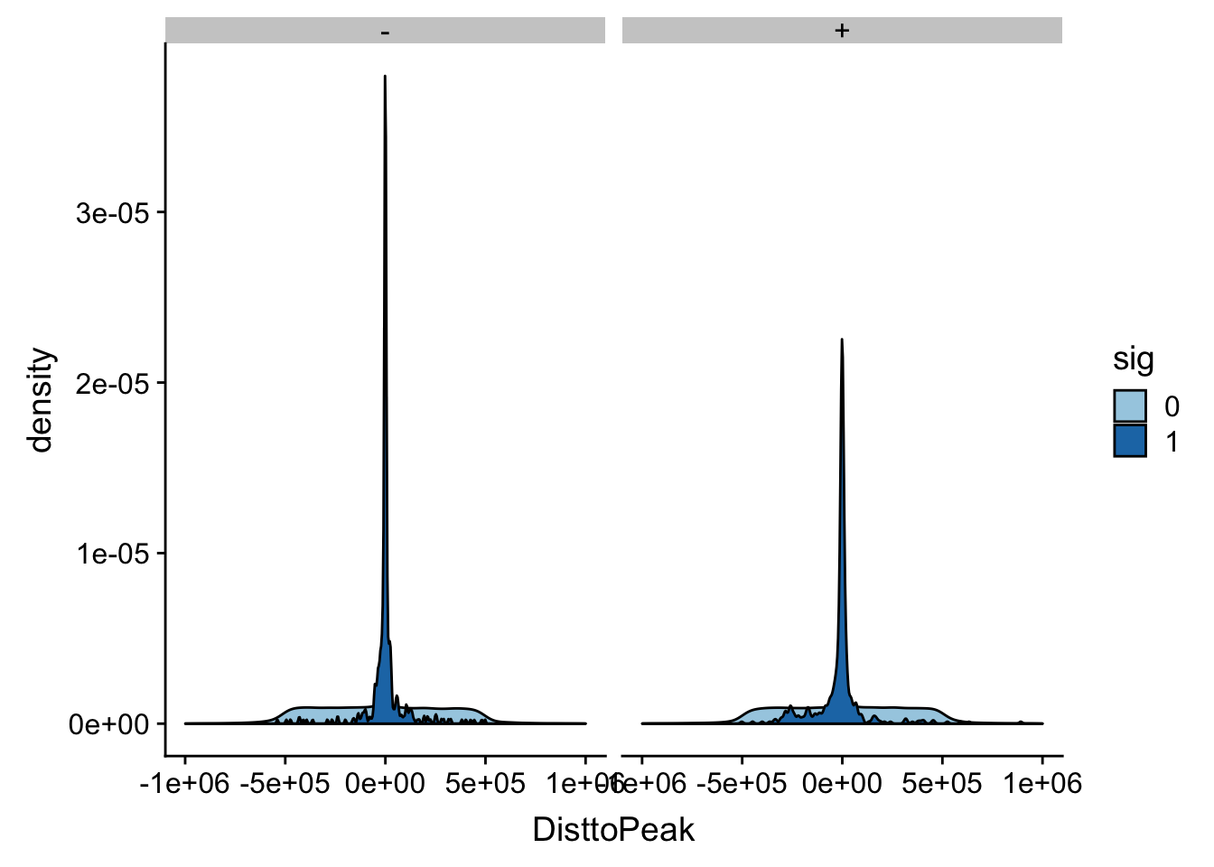
Expand here to see past versions of unnamed-chunk-10-2.png:
| Version | Author | Date |
|---|---|---|
| de860f0 | Briana Mittleman | 2018-10-24 |
I am going to plot a violin plot for just the significant ones.
ggplot(NuclearAPA_peakdist_sig, aes(x=DisttoPeak)) + geom_density(fill="deepskyblue3")+ labs(title="Nuclear: Distance from QTL to PAS Peak", x="Distance from SNP to PAS")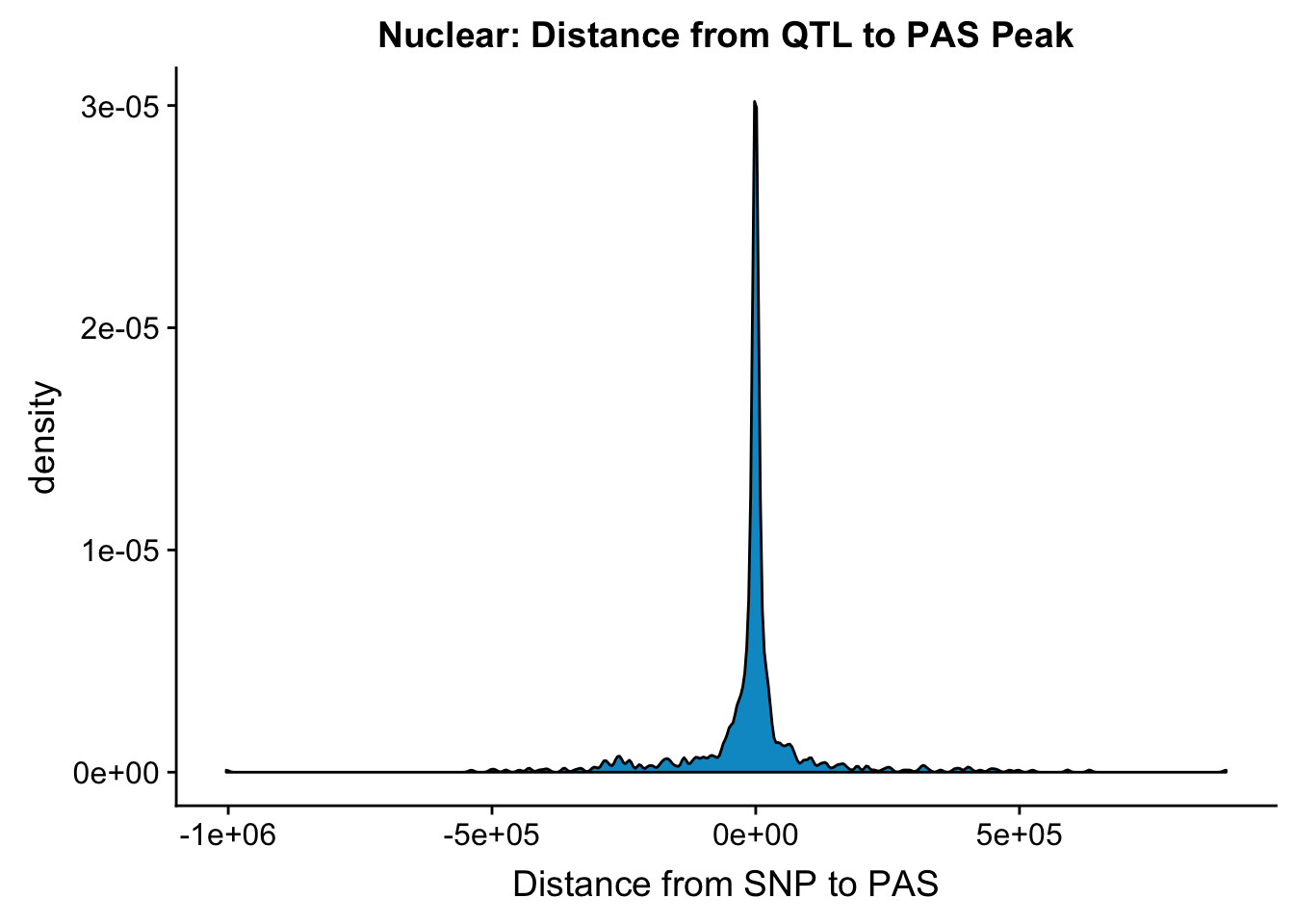
Expand here to see past versions of unnamed-chunk-11-1.png:
| Version | Author | Date |
|---|---|---|
| de860f0 | Briana Mittleman | 2018-10-24 |
Within 1000 bases of the peak center.
NuclearAPA_peakdist_sig %>% filter(abs(DisttoPeak) < 1000) %>% nrow()[1] 192NuclearAPA_peakdist_sig %>% filter(abs(DisttoPeak) < 10000) %>% nrow()[1] 420NuclearAPA_peakdist_sig %>% filter(abs(DisttoPeak) < 100000) %>% nrow()[1] 726192 QTLs are within 1000 bp, 420 are within 10000, and 726 are within 100,000bp
Expression metrics
Next I want to pull in the expression values and compare the expression of genes with a nuclear APA qtl in comparison to genes without one. I will also need to pull in the gene names file to add in the gene names from the ensg ID.
Remove the # from the file.
expression=read.table("../data/mol_pheno/fastqtl_qqnorm_RNAseq_phase2.fixed.noChr.txt", header = T,stringsAsFactors = F)
expression_mean=apply(expression[,5:73],1,mean,na.rm=TRUE)
expression_var=apply(expression[,5:73],1,var,na.rm=TRUE)
expression$exp.mean= expression_mean
expression$exp.var=expression_var
expression= expression %>% separate(ID, into=c("Gene.stable.ID", "ver"), sep ="[.]")
Now I can pull in the names and join the dataframes.
geneNames=read.table("../data/ensemble_to_genename.txt", sep="\t", header=T,stringsAsFactors = F)

expression=expression %>% inner_join(geneNames,by="Gene.stable.ID")

expression=expression %>% select(Chr, start, end, Gene.name, exp.mean,exp.var) %>%  rename("gene"=Gene.name)
Now I can join this with the qtls.
NuclearAPA_wExp=NuclearAPA %>% inner_join(expression, by="gene") gene_wQTL_N= NuclearAPA_wExp %>% group_by(gene) %>% summarise(sig_gene=sum(as.numeric(as.character(sig)))) %>% ungroup() %>% inner_join(expression, by="gene") %>% mutate(sigGeneFactor=ifelse(sig_gene>=1, 1,0))
gene_wQTL_N$sigGeneFactor= as.factor(as.character(gene_wQTL_N$sigGeneFactor))
summary(gene_wQTL_N$sigGeneFactor) 0 1
4589 607 There are 607 genes with a QTL
ggplot(gene_wQTL_N, aes(x=exp.mean, by=sigGeneFactor, fill=sigGeneFactor)) + geom_density(alpha=.3) +labs(title="Mean in RNA expression by genes with significant QTL", x="Mean in normalized expression") + scale_fill_discrete(guide = guide_legend(title = "Significant QTL"))+ scale_fill_brewer(palette="Paired")Scale for 'fill' is already present. Adding another scale for 'fill',
which will replace the existing scale.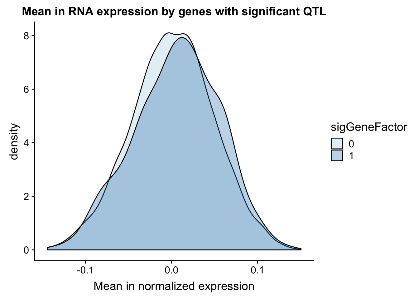
Expand here to see past versions of unnamed-chunk-17-1.png:
| Version | Author | Date |
|---|---|---|
| de860f0 | Briana Mittleman | 2018-10-24 |
I can do a similar analysis but test the variance in the gene expression.
ggplot(gene_wQTL_N, aes(x=exp.var, by=sigGeneFactor, fill=sigGeneFactor)) + geom_density(alpha=.3) + labs(title="Varriance in RNA expression by genes with significant QTL", x="Variance in normalized expression") + scale_fill_discrete(guide = guide_legend(title = "Significant QTL"))+ scale_fill_brewer(palette="Paired")Scale for 'fill' is already present. Adding another scale for 'fill',
which will replace the existing scale.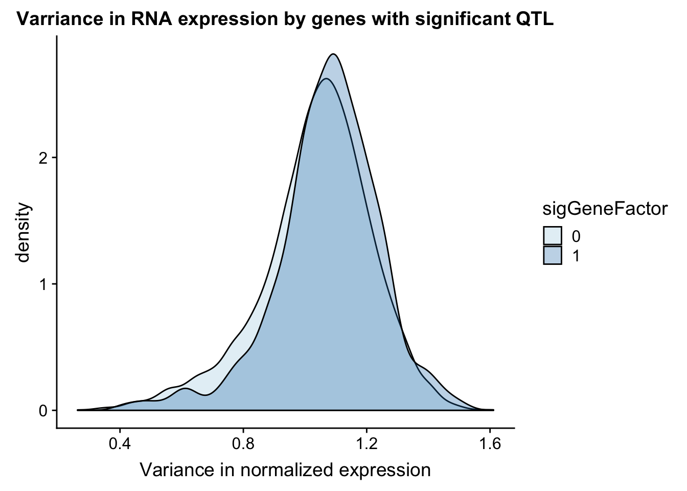
Expand here to see past versions of unnamed-chunk-18-1.png:
| Version | Author | Date |
|---|---|---|
| de860f0 | Briana Mittleman | 2018-10-24 |
Peak coverage for QTLs
I can also look at peak coverage for peaks with QLTs and those without. I will first look at this on peak level then mvoe to gene level. The peak scores come from the coverage in the peaks.
The NuclearAPA_peakdist data frame has the information I need for this.
ggplot(NuclearAPA_peakdist, aes(x=PeakScore,fill=sig,by=sig)) + geom_density(alpha=.5)+ scale_x_log10() + labs(title="Peak score by significance") + scale_fill_brewer(palette="Paired")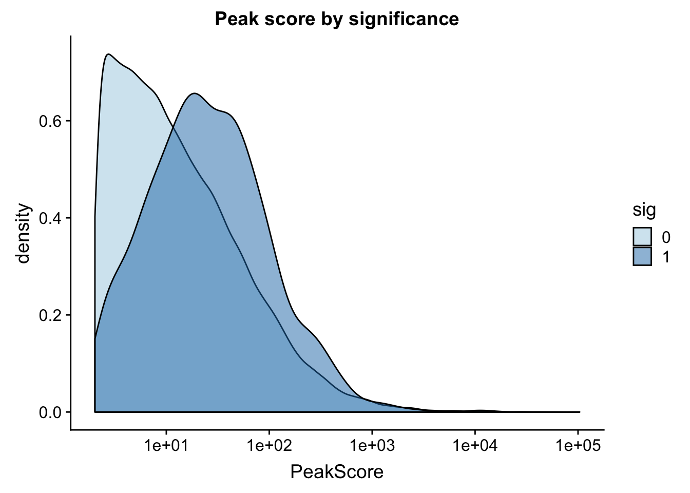
Expand here to see past versions of unnamed-chunk-19-1.png:
| Version | Author | Date |
|---|---|---|
| de860f0 | Briana Mittleman | 2018-10-24 |
This is expected. It makes sense that we have more power to detect qtls in higher expressed peaks. This leads me to believe that filtering out low peaks may add power but will not mitigate the effect. ##Where are the SNPs
I created the significant SNP files in the Characterize Total APAqtl analysis analysis.
chromHmm=read.table("../data/ChromHmmOverlap/chromHMM_regions.txt", col.names = c("number", "name"), stringsAsFactors = F)

NuclearOverlapHMM=read.table("../data/ChromHmmOverlap/Nuc_overlapHMM.bed", col.names=c("chrom", "start", "end", "sid", "significance", "strand", "number"))
NuclearOverlapHMM$number=as.integer(NuclearOverlapHMM$number)
NuclearOverlapHMM_names=NuclearOverlapHMM %>% left_join(chromHmm, by="number")
ggplot(NuclearOverlapHMM_names, aes(x=name)) + geom_bar() + labs(title="ChromHMM labels for Nuclear APAQtls" , y="Number of SNPs", x="Region")+theme(axis.text.x = element_text(angle = 90, hjust = 1))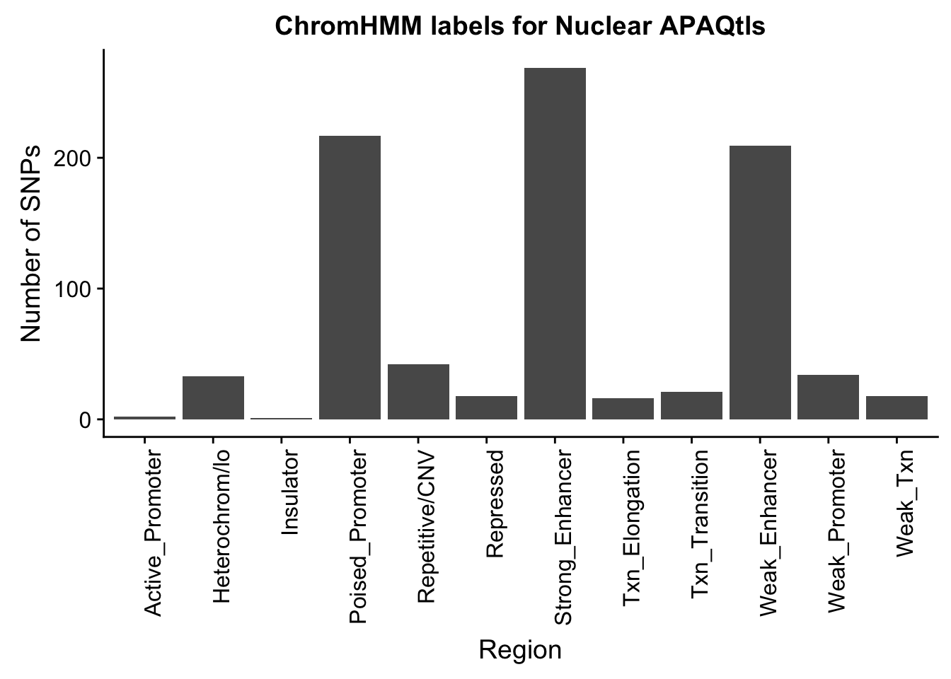
Expand here to see past versions of unnamed-chunk-21-1.png:
| Version | Author | Date |
|---|---|---|
| de860f0 | Briana Mittleman | 2018-10-24 |
I do still need to get 880 random snps.
shuf -n 880 /project2/gilad/briana/threeprimeseq/data/nominal_APAqtl_trans/filtered_APApeaks_merged_allchrom_refseqGenes_pheno_Nuclear_NomRes.txt > /project2/gilad/briana/threeprimeseq/data/nominal_APAqtl_trans/randomSnps/ApaQTL_nuclear_Random880.txt
Run QTLNOMres2SigSNPbed.py with nuclear 880 and sort output
import pybedtools

RANDnuc=pybedtools.BedTool('/project2/gilad/briana/threeprimeseq/data/nominal_APAqtl_trans/randomSnps/ApaQTL_nuclear_Random880.sort.bed')


hmm=pybedtools.BedTool("/project2/gilad/briana/genome_anotation_data/GM12878.chromHMM.sort.bed")

#map hmm to snps
NucRnad_overlapHMM=RANDnuc.map(hmm, c=4)


#save results

NucRnad_overlapHMM.saveas("/project2/gilad/briana/threeprimeseq/data/nominal_APAqtl_trans/randomSnps/ApaQTL_nuclear_Random_overlapHMM.bed")
NuclearRandOverlapHMM=read.table("../data/ChromHmmOverlap/ApaQTL_nuclear_Random_overlapHMM.bed", col.names=c("chrom", "start", "end", "sid", "significance", "strand", "number"))

NuclearRandOverlapHMM_names=NuclearRandOverlapHMM %>% left_join(chromHmm, by="number")
ggplot(NuclearRandOverlapHMM_names, aes(x=name)) + geom_bar() + labs(title="ChromHMM labels for Nuclear APAQtls (Random)" , y="Number of SNPs", x="Region")+theme(axis.text.x = element_text(angle = 90, hjust = 1))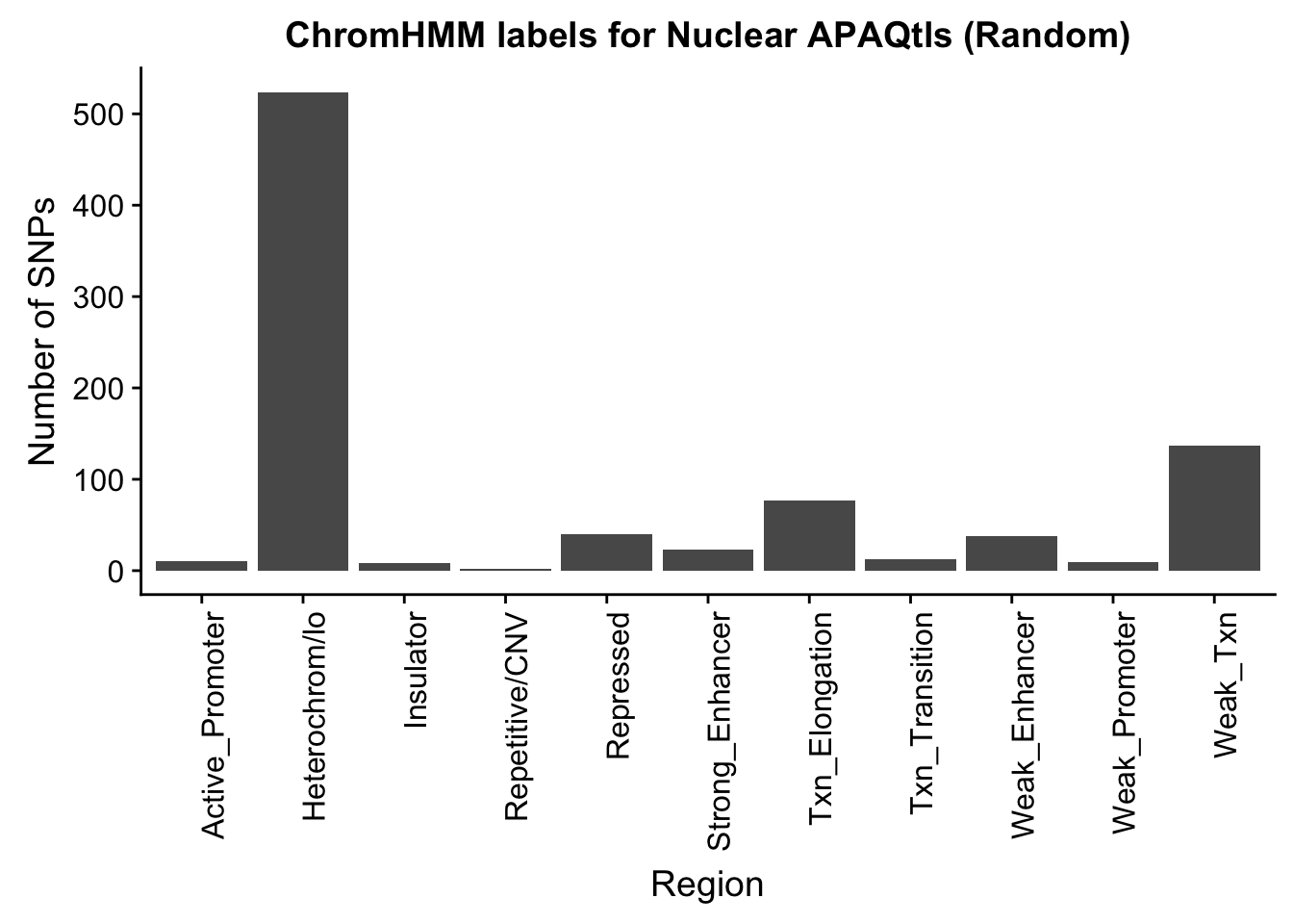
Expand here to see past versions of unnamed-chunk-25-1.png:
| Version | Author | Date |
|---|---|---|
| de860f0 | Briana Mittleman | 2018-10-24 |
To put this on the same plot I can count the number in each then plot them next to eachother.
random_perChromHMM_nuc=NuclearRandOverlapHMM_names %>%  group_by(name) %>% summarise(Random=n())
sig_perChromHMM_nuc= NuclearOverlapHMM_names %>%  group_by(name) %>%  summarise(Nuclear_QTLs=n())

perChrommHMM_nuc=random_perChromHMM_nuc %>%  full_join(sig_perChromHMM_nuc, by="name", ) %>% replace_na(list(Random=0,Total_QTLs=0))

perChrommHMM_nuc_melt=melt(perChrommHMM_nuc, id.vars="name")
names(perChrommHMM_nuc_melt)=c("Region","Set", "N_Snps" )
chromenrichNuclearplot=ggplot(perChrommHMM_nuc_melt, aes(x=Region, y=N_Snps, by=Set, fill=Set)) + geom_bar(position="dodge", stat="identity") +theme(axis.text.x = element_text(angle = 90, hjust = 1)) + labs(title="Enrichment of Nuclear QTLs by chromatin region", y="Number of Snps", x="Chromatin Region") + scale_fill_brewer(palette="Paired")
chromenrichNuclearplot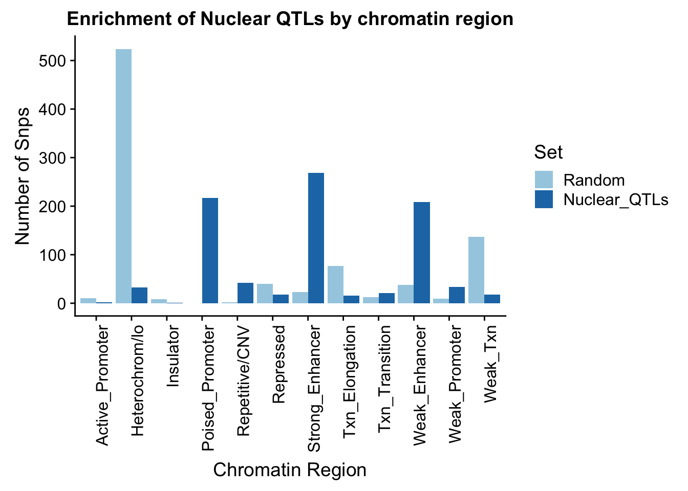
Expand here to see past versions of unnamed-chunk-27-1.png:
| Version | Author | Date |
|---|---|---|
| de860f0 | Briana Mittleman | 2018-10-24 |
ggsave("../output/plots/ChromHmmEnrich_Nuclear.png", chromenrichNuclearplot)Saving 7 x 5 in imageChompare enrichment between fractions
I want to make a plot with the enrichment by fraction. I am first going to get an enrichemnt score for each bin naively by looking at the QTL/random in each category.
perChrommHMM_nuc$Random= as.integer(perChrommHMM_nuc$Random)
perChrommHMM_nuc_enr=perChrommHMM_nuc %>%  mutate(Nuclear=Nuclear_QTLs-Random)

perChrommHMM_tot_enr=read.table("../data/ChromHmmOverlap/perChrommHMM_Total_enr.txt",stringsAsFactors = F,header = T)
allenrich=perChrommHMM_tot_enr %>% inner_join(perChrommHMM_nuc_enr, by="name") %>% select(name, Total, Nuclear)
allenrich_melt=melt(allenrich, id.vars="name")plot it
chromenrichBoth=ggplot(allenrich_melt, aes(x=name, by=variable, y=value, fill=variable)) + geom_bar(stat="identity", position = "dodge") + theme(axis.text.x = element_text(angle = 90, hjust = 1)) + labs(title="QTL-Random for each bin by fraction", y="Num QTL SNPs - Num Random SNPs") + scale_fill_manual(values=c("darkviolet", "deepskyblue3"))


ggsave("../output/plots/ChromHmmEnrich_BothFrac.png", chromenrichBoth)
Saving 7 x 5 in imagePermutations
I want to permute the background snps so i can get a better expectation. To do this I need to chose random lines from the nominal file, change the lines to snp format, overlap with HMM, count how many are in each category, and append the list to a dataframe that is category by permuation. I will do all of this in python.
def main(inFile, outFile, nperm,nsamp):
  nom_res= pd.read_csv(inFile, sep="\t", encoding="utf-8",header=None)
  out=open(outFile, "w")
  categories=list(range(1,16))
  out.write(" ".join(categories)+'\n')

  def make_rand_snp(x):
    #x is from the random snps pulled from the nom_res, return the snp df
    chrom_list=list()
    start_list=list()
    end_list=list()
    name_list=list()
    pval_list=list()
    strand_list=list()
    for ln in x:
          pid, sid, dist, pval, slope = ln.split()
          chrom, pos= sid.split(":")
          name=sid
          start= int(pos)-1
          end=int(pos)
          strand=pid.split(":")[3].split("_")[1]
          pval=float(pval)
          chrom_list.append(chrom)
          start_list.append(start)
          end_list.append(end)
          name_list.append(name)
          pval_list.append(pval)
          strand_list.append(strand)
          # add info to the lists
    #zip lists
    zip_list=list(zip(chrom_list,start_list,end_list,name_list,pval_list, strand_list))
    snp_df=pd.DataFrame(data=zip_list, columns=["Chrom", "Start", "End", "Name", "Pval", "Strand"])
    return snp_df

  for i in range(1, nperm+1):
    sample=nom_res.sample(nsamp)
    sample_snp=make_rand_snp(sample)
    sample_snp_sort=sample_snp.sort_values(by=['Chrom', 'Start'])
    hmm=pybedtools.BedTool("/project2/gilad/briana/genome_anotation_data/GM12878.chromHMM.sort.bed")
    sample_snp_bed=pybedtools.from_dataframe(sample_snp_sort)
    samp_overHMM=sample_snp_bed(hmm, c=4)
    samp_overHMM_df=pybedtools.to_dataframe(samp_overHMM,names=["chrom", "start", "end", "sid", "significance", "strand", "number"])
    samp_overHMM_df.groupby('number').count()
    #need to see how this comes out and how I can make it into a list, after i have the list for each I can zip them together (list_i)

if __name__ == "__main__":
    import sys
    import pybedtools
    import pandas as pd
    fraction = sys.argv[1]
    nperm= sys.argv[2]
    nperm=int(nperm)
    nsamp=sys.argv[3]
    nsamp=int(nsamp)
    inFile = "/project2/gilad/briana/threeprimeseq/data/nominal_APAqtl_trans/filtered_APApeaks_merged_allchrom_refseqGenes_pheno_%s_NomRes.txt"%(fraction)
    outFile = "dataframe with res"%()
    main(inFile, outFile, nperm, nsamp)
Maybe it is better to make this a bash script that has a pipeline of different scripts. This way I wont have to worry about files/dataframes and all of that.
DO this for total first (118 snps)
total_random118_chromHmm.sh
#!/bin/bash

#SBATCH --job-name=total_random118_chromHmm
#SBATCH --account=pi-yangili1
#SBATCH --time=36:00:00
#SBATCH --output=total_random118_chromHmm.out
#SBATCH --error=total_random118_chromHmm.err
#SBATCH --partition=bigmem2
#SBATCH --mem=200G
#SBATCH --mail-type=END

module load Anaconda3
source activate three-prime-env


#test with 2 permutations then make it 1000
#choose random res
for i in {1..100};
do
shuf -n 118 /project2/gilad/briana/threeprimeseq/data/nominal_APAqtl_trans/filtered_APApeaks_merged_allchrom_refseqGenes_pheno_Total_NomRes.txt > /project2/gilad/briana/threeprimeseq/data/random_QTLsnps/Nuclear/randomRes_Total_118_${i}.txt
done

#make random
for i in {1..1000};
do
python randomRes2SNPbed.py Total 118 ${i}
done


#cat res together
cat /project2/gilad/briana/threeprimeseq/data/random_QTLsnps/Total/snp_bed/* > /project2/gilad/briana/threeprimeseq/data/random_QTLsnps/Total/snp_bed_all/randomRes_Total_118_ALLperm.bed


#sort full file
sort -k1,1 -k2,2n /project2/gilad/briana/threeprimeseq/data/random_QTLsnps/Total/snp_bed_all/randomRes_Total_118_ALLperm.bed > /project2/gilad/briana/threeprimeseq/data/random_QTLsnps/Total/snp_bed_all/randomRes_Total_118_ALLperm.sort.bed


#hmm overlap
python overlap_chromHMM.py  Total 118 1000

#Next I would pull this into R to do the group by and average!
pull_random_lines.py
def main(inFile, outFile ,nsamp):
  nom_res= pd.read_csv(inFile, sep="\t", encoding="utf-8",header=None)
  out=open(outFile, "w")
  sample=nom_res.sample(nsamp)
  sample.to_csv(out, sep="\t", encoding='utf-8', index=False, header=F)
  out.close()

if __name__ == "__main__":
    import sys
    import pandas as pd
    fraction = sys.argv[1]
    nsamp=sys.argv[2]
    nsamp=int(nsamp)
    iter=sys.argv[3]
    inFile = "/project2/gilad/briana/threeprimeseq/data/nominal_APAqtl_trans/filtered_APApeaks_merged_allchrom_refseqGenes_pheno_%s_NomRes.txt"%(fraction)
    outFile = "/project2/gilad/briana/threeprimeseq/data/random_QTLsnps/%s/randomRes_%s_%d_%s.txt"%(fraction,fraction, nsamp, iter)
    main(inFile, outFile, nsamp)
randomRes2SNPbed.py
def main(inFile, outFile):
    fout=open(outFile, "w")
    fin=open(inFile, "r")
    for ln in fin:
          pid, sid, dist, pval, slope = ln.split()
          chrom, pos= sid.split(":")
          name=sid
          start= int(pos)-1
          end=int(pos)
          strand=pid.split(":")[3].split("_")[1]
          pval=float(pval)
          fout.write("%s\t%s\t%s\t%s\t%s\t%s\n"%(chrom, start, end, name, pval, strand))
    fout.close()

if __name__ == "__main__":
    import sys
    fraction=sys.argv[1]
    nsamp=sys.argv[2]
    nsamp=int(nsamp)
    iter=sys.argv[3]
    inFile = "/project2/gilad/briana/threeprimeseq/data/random_QTLsnps/%s/randomRes_%s_%d_%s.txt"%(fraction,fraction, nsamp, iter)
    outFile= "/project2/gilad/briana/threeprimeseq/data/random_QTLsnps/%s/snp_bed/randomRes_%s_%d_%s.bed"%(fraction,fraction, nsamp, iter)
    main(inFile,outFile)
overlap_chromHMM.py
def main(inFile, outFile):
  rand=pybedtools.BedTool(inFile)
  hmm=pybedtools.BedTool("/project2/gilad/briana/genome_anotation_data/GM12878.chromHMM.sort.bed")
  #map hmm to snps
  Rand_overlapHMM=rand.map(hmm, c=4)
  #save results
  Rand_overlapHMM.saveas(outFile)


if __name__ == "__main__":
    import sys
    import pandas as pd
    import pybedtools
    fraction=sys.argv[1]
    nsamp=sys.argv[2]
    niter=sys.argv[3]
    inFile = "/project2/gilad/briana/threeprimeseq/data/random_QTLsnps/%s/snp_bed_all/randomRes_%s_%s_ALLperm.sort.bed"%(fraction,fraction, nsamp)
    outFile= "/project2/gilad/briana/threeprimeseq/data/random_QTLsnps/%s/chromHMM_overlap/randomres_overlapChromHMM_%s_%s_%s.txt"%(fraction,fraction,nsamp, niter)
    main(inFile,outFile)
*Nuclear 880
nuclear_random880_chromHmm.sh
#!/bin/bash

#SBATCH --job-name=nuc_random880_chromHmm
#SBATCH --account=pi-yangili1
#SBATCH --time=36:00:00
#SBATCH --output=nuc_random880_chromHmm.out
#SBATCH --error=nuc_random880_chromHmm.err
#SBATCH --partition=bigmem2
#SBATCH --mem=200G
#SBATCH --mail-type=END

module load Anaconda3
source activate three-prime-env


#test with 2 permutations then make it 1000
#choose random res
for i in {1..1000};
do
shuf -n 880 /project2/gilad/briana/threeprimeseq/data/nominal_APAqtl_trans/filtered_APApeaks_merged_allchrom_refseqGenes_pheno_Nuclear_NomRes.txt > /project2/gilad/briana/threeprimeseq/data/random_QTLsnps/Nuclear/randomRes_Nuclear_880_${i}.txt
done

#make random
for i in {1..1000};
do
python randomRes2SNPbed.py Nuclear 880 ${i}
done


#cat res together
cat /project2/gilad/briana/threeprimeseq/data/random_QTLsnps/Nuclear/snp_bed/* > /project2/gilad/briana/threeprimeseq/data/random_QTLsnps/Nuclear/snp_bed_all/randomRes_Nuclear_880_ALLperm.bed


#sort full file
sort -k1,1 -k2,2n /project2/gilad/briana/threeprimeseq/data/random_QTLsnps/Nuclear/snp_bed_all/randomRes_Nuclear_880_ALLperm.bed > /project2/gilad/briana/threeprimeseq/data/random_QTLsnps/Nuclear/snp_bed_all/randomRes_Nuclear_880_ALLperm.sort.bed


#hmm overlap
python overlap_chromHMM.py  Nuclear 880 1000

#Next I would pull this into R to do the group by and average!
Session information
sessionInfo()R version 3.5.1 (2018-07-02)
Platform: x86_64-apple-darwin15.6.0 (64-bit)
Running under: macOS Sierra 10.12.6
Matrix products: default
BLAS: /Library/Frameworks/R.framework/Versions/3.5/Resources/lib/libRblas.0.dylib
LAPACK: /Library/Frameworks/R.framework/Versions/3.5/Resources/lib/libRlapack.dylib
locale:
[1] en_US.UTF-8/en_US.UTF-8/en_US.UTF-8/C/en_US.UTF-8/en_US.UTF-8
attached base packages:
[1] grid stats graphics grDevices utils datasets methods
[8] base
other attached packages:
[1] bindrcpp_0.2.2 cowplot_0.9.3 data.table_1.11.8
[4] VennDiagram_1.6.20 futile.logger_1.4.3 forcats_0.3.0
[7] stringr_1.3.1 dplyr_0.7.6 purrr_0.2.5
[10] readr_1.1.1 tidyr_0.8.1 tibble_1.4.2
[13] ggplot2_3.0.0 tidyverse_1.2.1 reshape2_1.4.3
[16] workflowr_1.1.1
loaded via a namespace (and not attached):
[1] tidyselect_0.2.4 haven_1.1.2 lattice_0.20-35
[4] colorspace_1.3-2 htmltools_0.3.6 yaml_2.2.0
[7] rlang_0.2.2 R.oo_1.22.0 pillar_1.3.0
[10] glue_1.3.0 withr_2.1.2 R.utils_2.7.0
[13] RColorBrewer_1.1-2 lambda.r_1.2.3 modelr_0.1.2
[16] readxl_1.1.0 bindr_0.1.1 plyr_1.8.4
[19] munsell_0.5.0 gtable_0.2.0 cellranger_1.1.0
[22] rvest_0.3.2 R.methodsS3_1.7.1 evaluate_0.11
[25] labeling_0.3 knitr_1.20 broom_0.5.0
[28] Rcpp_0.12.19 formatR_1.5 backports_1.1.2
[31] scales_1.0.0 jsonlite_1.5 hms_0.4.2
[34] digest_0.6.17 stringi_1.2.4 rprojroot_1.3-2
[37] cli_1.0.1 tools_3.5.1 magrittr_1.5
[40] lazyeval_0.2.1 futile.options_1.0.1 crayon_1.3.4
[43] whisker_0.3-2 pkgconfig_2.0.2 xml2_1.2.0
[46] lubridate_1.7.4 assertthat_0.2.0 rmarkdown_1.10
[49] httr_1.3.1 rstudioapi_0.8 R6_2.3.0
[52] nlme_3.1-137 git2r_0.23.0 compiler_3.5.1
This reproducible R Markdown analysis was created with workflowr 1.1.1