PacPio Reads in my peaks
Briana Mittleman
2/26/2019
Last updated: 2019-02-27
Checks: 6 0
Knit directory: threeprimeseq/analysis/
This reproducible R Markdown analysis was created with workflowr (version 1.2.0). The Report tab describes the reproducibility checks that were applied when the results were created. The Past versions tab lists the development history.
Great! Since the R Markdown file has been committed to the Git repository, you know the exact version of the code that produced these results.
Great job! The global environment was empty. Objects defined in the global environment can affect the analysis in your R Markdown file in unknown ways. For reproduciblity it’s best to always run the code in an empty environment.
The command set.seed(12345) was run prior to running the code in the R Markdown file. Setting a seed ensures that any results that rely on randomness, e.g. subsampling or permutations, are reproducible.
Great job! Recording the operating system, R version, and package versions is critical for reproducibility.
Nice! There were no cached chunks for this analysis, so you can be confident that you successfully produced the results during this run.
Great! You are using Git for version control. Tracking code development and connecting the code version to the results is critical for reproducibility. The version displayed above was the version of the Git repository at the time these results were generated.
Note that you need to be careful to ensure that all relevant files for the analysis have been committed to Git prior to generating the results (you can use wflow_publish or wflow_git_commit). workflowr only checks the R Markdown file, but you know if there are other scripts or data files that it depends on. Below is the status of the Git repository when the results were generated:
Ignored files:
    Ignored:    .DS_Store
    Ignored:    .Rhistory
    Ignored:    .Rproj.user/
    Ignored:    data/.DS_Store
    Ignored:    data/perm_QTL_trans_noMP_5percov/
    Ignored:    output/.DS_Store

Untracked files:
    Untracked:  KalistoAbundance18486.txt
    Untracked:  analysis/4suDataIGV.Rmd
    Untracked:  analysis/DirectionapaQTL.Rmd
    Untracked:  analysis/EvaleQTLs.Rmd
    Untracked:  analysis/YL_QTL_test.Rmd
    Untracked:  analysis/fixBWChromNames.Rmd
    Untracked:  analysis/groSeqAnalysis.Rmd
    Untracked:  analysis/ncbiRefSeq_sm.sort.mRNA.bed
    Untracked:  analysis/snake.config.notes.Rmd
    Untracked:  analysis/verifyBAM.Rmd
    Untracked:  analysis/verifybam_dubs.Rmd
    Untracked:  code/PeaksToCoverPerReads.py
    Untracked:  code/strober_pc_pve_heatmap_func.R
    Untracked:  data/18486.genecov.txt
    Untracked:  data/APApeaksYL.total.inbrain.bed
    Untracked:  data/AllPeak_counts/
    Untracked:  data/ApaQTLs/
    Untracked:  data/ApaQTLs_otherPhen/
    Untracked:  data/ChromHmmOverlap/
    Untracked:  data/DistTXN2Peak_genelocAnno/
    Untracked:  data/GM12878.chromHMM.bed
    Untracked:  data/GM12878.chromHMM.txt
    Untracked:  data/LianoglouLCL/
    Untracked:  data/LocusZoom/
    Untracked:  data/LocusZoom_Unexp/
    Untracked:  data/LocusZoom_proc/
    Untracked:  data/MatchedSnps/
    Untracked:  data/NuclearApaQTLs.txt
    Untracked:  data/PeakCounts/
    Untracked:  data/PeakCounts_noMP_5perc/
    Untracked:  data/PeakCounts_noMP_genelocanno/
    Untracked:  data/PeakUsage/
    Untracked:  data/PeakUsage_noMP/
    Untracked:  data/PeakUsage_noMP_GeneLocAnno/
    Untracked:  data/PeaksUsed/
    Untracked:  data/PeaksUsed_noMP_5percCov/
    Untracked:  data/QTL_overlap/
    Untracked:  data/RNAkalisto/
    Untracked:  data/RefSeq_annotations/
    Untracked:  data/Replicates_usage/
    Untracked:  data/TotalApaQTLs.txt
    Untracked:  data/Totalpeaks_filtered_clean.bed
    Untracked:  data/UnderstandPeaksQC/
    Untracked:  data/WASP_STAT/
    Untracked:  data/YL-SP-18486-T-combined-genecov.txt
    Untracked:  data/YL-SP-18486-T_S9_R1_001-genecov.txt
    Untracked:  data/YL_QTL_test/
    Untracked:  data/apaExamp/
    Untracked:  data/apaExamp_proc/
    Untracked:  data/apaQTL_examp_noMP/
    Untracked:  data/bedgraph_peaks/
    Untracked:  data/bin200.5.T.nuccov.bed
    Untracked:  data/bin200.Anuccov.bed
    Untracked:  data/bin200.nuccov.bed
    Untracked:  data/clean_peaks/
    Untracked:  data/comb_map_stats.csv
    Untracked:  data/comb_map_stats.xlsx
    Untracked:  data/comb_map_stats_39ind.csv
    Untracked:  data/combined_reads_mapped_three_prime_seq.csv
    Untracked:  data/diff_iso_GeneLocAnno/
    Untracked:  data/diff_iso_proc/
    Untracked:  data/diff_iso_trans/
    Untracked:  data/eQTLs_Lietal/
    Untracked:  data/ensemble_to_genename.txt
    Untracked:  data/example_gene_peakQuant/
    Untracked:  data/explainProtVar/
    Untracked:  data/filtPeakOppstrand_cov_noMP_GeneLocAnno_5perc/
    Untracked:  data/filtered_APApeaks_merged_allchrom_refseqTrans.closest2End.bed
    Untracked:  data/filtered_APApeaks_merged_allchrom_refseqTrans.closest2End.noties.bed
    Untracked:  data/first50lines_closest.txt
    Untracked:  data/gencov.test.csv
    Untracked:  data/gencov.test.txt
    Untracked:  data/gencov_zero.test.csv
    Untracked:  data/gencov_zero.test.txt
    Untracked:  data/gene_cov/
    Untracked:  data/joined
    Untracked:  data/leafcutter/
    Untracked:  data/merged_combined_YL-SP-threeprimeseq.bg
    Untracked:  data/molPheno_noMP/
    Untracked:  data/mol_overlap/
    Untracked:  data/mol_pheno/
    Untracked:  data/nom_QTL/
    Untracked:  data/nom_QTL_opp/
    Untracked:  data/nom_QTL_trans/
    Untracked:  data/nuc6up/
    Untracked:  data/nuc_10up/
    Untracked:  data/other_qtls/
    Untracked:  data/pQTL_otherphen/
    Untracked:  data/pacbio_cov/
    Untracked:  data/peakPerRefSeqGene/
    Untracked:  data/perm_QTL/
    Untracked:  data/perm_QTL_GeneLocAnno_noMP_5percov/
    Untracked:  data/perm_QTL_GeneLocAnno_noMP_5percov_3UTR/
    Untracked:  data/perm_QTL_diffWindow/
    Untracked:  data/perm_QTL_opp/
    Untracked:  data/perm_QTL_trans/
    Untracked:  data/perm_QTL_trans_filt/
    Untracked:  data/protAndAPAAndExplmRes.Rda
    Untracked:  data/protAndAPAlmRes.Rda
    Untracked:  data/protAndExpressionlmRes.Rda
    Untracked:  data/reads_mapped_three_prime_seq.csv
    Untracked:  data/smash.cov.results.bed
    Untracked:  data/smash.cov.results.csv
    Untracked:  data/smash.cov.results.txt
    Untracked:  data/smash_testregion/
    Untracked:  data/ssFC200.cov.bed
    Untracked:  data/temp.file1
    Untracked:  data/temp.file2
    Untracked:  data/temp.gencov.test.txt
    Untracked:  data/temp.gencov_zero.test.txt
    Untracked:  data/threePrimeSeqMetaData.csv
    Untracked:  data/threePrimeSeqMetaData55Ind.txt
    Untracked:  data/threePrimeSeqMetaData55Ind.xlsx
    Untracked:  data/threePrimeSeqMetaData55Ind_noDup.txt
    Untracked:  data/threePrimeSeqMetaData55Ind_noDup.xlsx
    Untracked:  data/threePrimeSeqMetaData55Ind_noDup_WASPMAP.txt
    Untracked:  data/threePrimeSeqMetaData55Ind_noDup_WASPMAP.xlsx
    Untracked:  output/LZ/
    Untracked:  output/deeptools_plots/
    Untracked:  output/picard/
    Untracked:  output/plots/
    Untracked:  output/qual.fig2.pdf

Unstaged changes:
    Modified:   analysis/28ind.peak.explore.Rmd
    Modified:   analysis/CompareLianoglouData.Rmd
    Modified:   analysis/NewPeakPostMP.Rmd
    Modified:   analysis/apaQTLoverlapGWAS.Rmd
    Modified:   analysis/cleanupdtseq.internalpriming.Rmd
    Modified:   analysis/coloc_apaQTLs_protQTLs.Rmd
    Modified:   analysis/dif.iso.usage.leafcutter.Rmd
    Modified:   analysis/diffIsoAnalysisNewMapping.Rmd
    Modified:   analysis/diff_iso_pipeline.Rmd
    Modified:   analysis/explainpQTLs.Rmd
    Modified:   analysis/explore.filters.Rmd
    Modified:   analysis/flash2mash.Rmd
    Modified:   analysis/mispriming_approach.Rmd
    Modified:   analysis/overlapMolQTL.Rmd
    Modified:   analysis/overlapMolQTL.opposite.Rmd
    Modified:   analysis/overlap_qtls.Rmd
    Modified:   analysis/peakOverlap_oppstrand.Rmd
    Modified:   analysis/peakQCPPlots.Rmd
    Modified:   analysis/pheno.leaf.comb.Rmd
    Modified:   analysis/pipeline_55Ind.Rmd
    Modified:   analysis/swarmPlots_QTLs.Rmd
    Modified:   analysis/test.max2.Rmd
    Modified:   analysis/test.smash.Rmd
    Modified:   analysis/understandPeaks.Rmd
    Modified:   analysis/unexplainedeQTL_analysis.Rmd
    Modified:   code/Snakefile
Note that any generated files, e.g. HTML, png, CSS, etc., are not included in this status report because it is ok for generated content to have uncommitted changes.
These are the previous versions of the R Markdown and HTML files. If you’ve configured a remote Git repository (see ?wflow_git_remote), click on the hyperlinks in the table below to view them.
| File | Version | Author | Date | Message |
|---|---|---|---|---|
| Rmd | eb1a05c | Briana Mittleman | 2019-02-27 | add pacbio analysis |
| html | f832bb0 | Briana Mittleman | 2019-02-26 | Build site. |
| Rmd | 6637b21 | Briana Mittleman | 2019-02-26 | add avg total usage |
| html | b27ba86 | Briana Mittleman | 2019-02-26 | Build site. |
| Rmd | c5dfa4b | Briana Mittleman | 2019-02-26 | fix file for ankeeta |
library(workflowr)This is workflowr version 1.2.0
Run ?workflowr for help getting startedlibrary(tidyverse)── Attaching packages ─────────────────────────────────────────────────────────────────────────── tidyverse 1.2.1 ──✔ ggplot2 3.0.0 ✔ purrr 0.2.5
✔ tibble 1.4.2 ✔ dplyr 0.7.6
✔ tidyr 0.8.1 ✔ stringr 1.4.0
✔ readr 1.1.1 ✔ forcats 0.3.0Warning: package 'stringr' was built under R version 3.5.2── Conflicts ────────────────────────────────────────────────────────────────────────────── tidyverse_conflicts() ──
✖ dplyr::filter() masks stats::filter()
✖ dplyr::lag() masks stats::lag()library(reshape2)
Attaching package: 'reshape2'The following object is masked from 'package:tidyr':
smithslibrary(cowplot)
Attaching package: 'cowplot'The following object is masked from 'package:ggplot2':
ggsaveAnkeeta has been working with 3 pac bio libraries for whole LCLs. The meged bam file has 4,164,259 reads. I want to look at how many of these reads cover my peaks. It would be best to know how many reads ends
I need to fix the strand for my peaks and give them to her.
fixPeaks4Ankeeta.py
In=open("/project2/gilad/briana/threeprimeseq/data/mergedPeaks_noMP_GeneLoc/Filtered_APApeaks_merged_allchrom_noMP.sort.named.noCHR_geneLocParsed_withAnno.SAF","r")
Out="/project2/yangili1/PAPeaks_STARMap_GeneLocAnno.bed"

def fix_strand(Fin,Fout):
    fout=open(Fout,"w")
    for n, ln in enumerate(Fin):
        if n == 0:
            continue
        else:
            id, chrom, start, end, strand = ln.split()
            if strand=="+":
                chromF="chr" + chrom
                peak=id.split(":")[0]
                geneLoc=id.split(":")[5:]
                geneLocF=":".join(geneLoc)
                newID=peak + ":" + geneLocF
                score="."
                fout.write("%s\t%s\t%s\t%s\t%s\t-\n"%(chromF,start,end,newID,score))
            else:
                chromF="chr" + chrom
                peak=id.split(":")[0]
                geneLoc=id.split(":")[5:]
                geneLocF=":".join(geneLoc)
                newID=peak + ":" + geneLocF
                score="."
                fout.write("%s\t%s\t%s\t%s\t%s\t+\n"%(chromF,start,end,newID,score))
    fout.close()


fix_strand(In, Out)
Add average usage to this:
use similar code to filter_5percUsagePeaks.R
counts only numeric are in /project2/gilad/briana/threeprimeseq/data/phenotypes_filtPeakTranscript_noMP_GeneLocAnno/filtered_APApeaks_merged_allchrom_refseqGenes.GeneLocAnno_NoMP_sm_quant.Total.fixed.pheno.CountsOnlyNumeric.txt I will take the mean for each row of this and use it as the score in the bed file.
Run this interactively
library(dplyr)
totUsage=read.table("/project2/gilad/briana/threeprimeseq/data/phenotypes_filtPeakTranscript_noMP_GeneLocAnno/filtered_APApeaks_merged_allchrom_refseqGenes.GeneLocAnno_NoMP_sm_quant.Total.fixed.pheno.CountsOnlyNumeric.txt", header=F)
peakBed=read.table("/project2/yangili1/PAPeaks_STARMap_GeneLocAnno.bed", header=F, col.names = c("chr", "start", "end", "ID", "score", "strand"), stringsAsFactors = F)


MeanUsage=rowMeans(totUsage)

outBed=as.data.frame(cbind(peakBed, MeanUsage)) %>% select(chr, start, end, ID, MeanUsage, strand)

write.table(outBed,file="/project2/yangili1/PAPeaks_STARMap_GeneLocAnno_withMeanUsage.bed", row.names=F, col.names=F, quote = F, sep="\t")
Result from pac bio overlap:
- /project2/yangili1/ankeetashah/APA_tools/peaks/threeprime_noMP_pacbio_UTR.coverage
- project2/yangili1/ankeetashah/APA_tools/peaks/threeprime_noMP_pacbio_intron.coverage
Make some plots for this: Distribution of reads ending at each peak
covNames=c("chr", "start", "end", "ID", "score", "strand", "cov")
utrCov=read.table("../data/pacbio_cov/threeprime_noMP_pacbio_UTR.coverage", stringsAsFactors = F, col.names = covNames)
intronCov=read.table("../data/pacbio_cov/threeprime_noMP_pacbio_intron.coverage", stringsAsFactors = F,col.names = covNames) %>% separate(ID, into=c("peak", "gene","loc"), sep=":") %>% filter(loc=="intron")
Plot the distributions:
ggplot(utrCov, aes(x=log10(cov + 1))) + geom_density() + labs(title="PacBio reads ending at each UTR peak", x="log10(nReads+1)")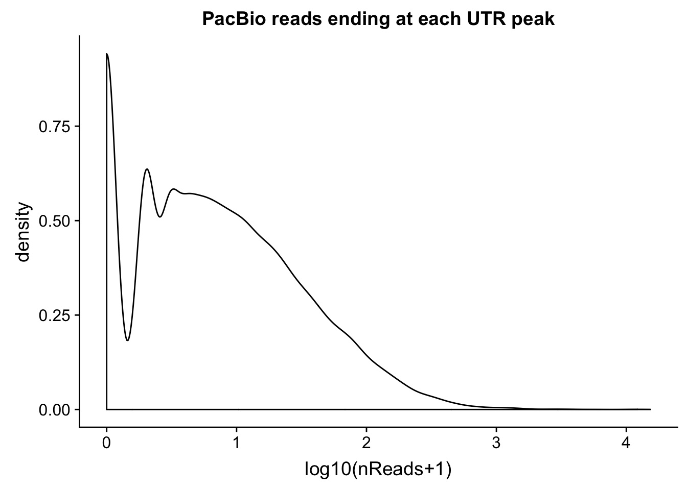
ggplot(intronCov, aes(x=log10(cov + 1))) + geom_density() + labs(title="PacBio reads ending at each intronic peak", x="log10(nReads+1)")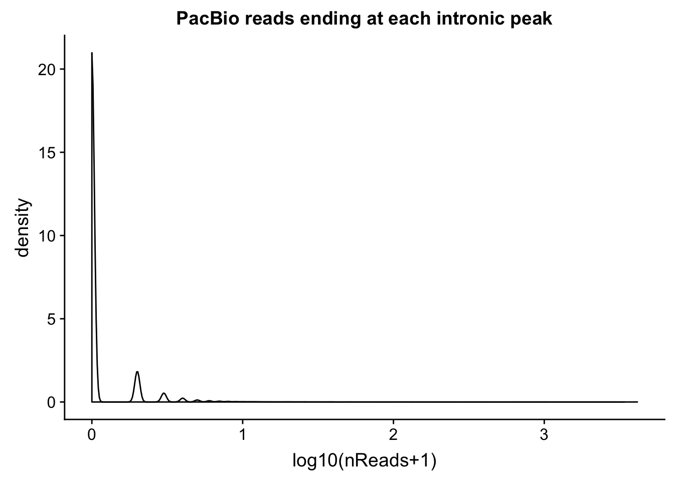
summary(intronCov$cov) Min. 1st Qu. Median Mean 3rd Qu. Max.
0.000 0.000 0.000 0.611 0.000 4145.000 summary(utrCov$cov) Min. 1st Qu. Median Mean 3rd Qu. Max.
0.00 1.00 5.00 24.93 18.00 15301.00 Proportion of peaks with coverage
intronCov_0=intronCov %>% filter(cov > 0) %>% nrow()/ nrow(intronCov)
intronCov_10=intronCov %>% filter(cov >= 10) %>% nrow()/nrow(intronCov)
intronCov_100=intronCov %>% filter(cov >= 100) %>% nrow()/nrow(intronCov)
intronCov_1000=intronCov %>% filter(cov >= 1000) %>% nrow()/nrow(intronCov)


utrCov_0=utrCov %>% filter(cov > 0) %>% nrow() / nrow(utrCov)
utrCov_10=utrCov %>% filter(cov >= 10) %>% nrow()/ nrow(utrCov)
utrCov_100=utrCov %>% filter(cov >= 100) %>% nrow()/ nrow(utrCov)
utrCov_1000=utrCov %>% filter(cov >= 1000) %>% nrow()/ nrow(utrCov)


Reads=c("1 read", "10 reads", "100 reads", "1000 reads")
UTR=c(utrCov_0, utrCov_10, utrCov_100, utrCov_1000)
Intron=c(intronCov_0,intronCov_10,intronCov_100,intronCov_1000)

covDF=as.data.frame(cbind(Reads,UTR,Intron))
covDF$UTR=as.numeric(as.character(covDF$UTR))
covDF$Intron=as.numeric(as.character(covDF$Intron))


covDF_melt=melt(covDF, id.vars = "Reads")
colnames(covDF_melt)=c("ReadCutoff", "Location", "Proportion" )
propcovbycutff=ggplot(covDF_melt, aes(x=ReadCutoff, fill=Location, y=Proportion, by=Location)) + geom_bar(position="dodge",stat="identity" ) + labs(y="Proportion of PAS covered", x="At least X reads ending at PAS", title="Proportion of PAS with PacBio read ending in it") + scale_fill_manual(values=c("blue","red")) + annotate("text", label="UTR PAS = 29,687", x="1000 reads", y=.7) + annotate("text", label="Intronic PAS = 87,733", x="1000 reads", y=.6)
propcovbycutff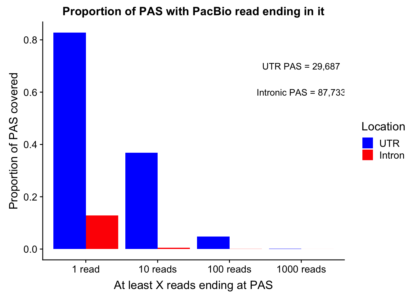
ggsave(propcovbycutff, filename = "../output/plots/PacBioReadsEndingAtPAS.png")Saving 7 x 5 in imageSubset for peaks that passed the 5% coverage cutoff.
tot5Perc=read.table("../data/PeakUsage_noMP_GeneLocAnno/filtered_APApeaks_merged_allchrom_refseqGenes.GeneLocAnno.NoMP_sm_quant.Total_fixed.pheno.5percPeaks.txt", stringsAsFactors = F, col.names = c("chr", "start", "end", "gene", "strand", "peak", "avgUsage"))
nuc5Perc=read.table("../data/PeakUsage_noMP_GeneLocAnno/filtered_APApeaks_merged_allchrom_refseqGenes.GeneLocAnno.NoMP_sm_quant.Nuclear_fixed.pheno.5percPeaks.txt",col.names = c("chr", "start", "end", "gene", "strand", "peak", "avgUsage"),stringsAsFactors = F)
intronCov_tot5perc= intronCov %>% semi_join(tot5Perc, by="peak")
intronCov_nuc5perc= intronCov %>% semi_join(nuc5Perc, by="peak")intronCov_tot5perc_0= intronCov_tot5perc %>% filter(cov> 0) %>% nrow()/ nrow(intronCov_tot5perc)
intronCov_tot5perc_10= intronCov_tot5perc %>% filter(cov>= 10) %>% nrow()/ nrow(intronCov_tot5perc)
intronCov_tot5perc_100= intronCov_tot5perc %>% filter(cov>= 100) %>% nrow()/ nrow(intronCov_tot5perc)
intronCov_tot5perc_1000= intronCov_tot5perc %>% filter(cov>= 1000) %>% nrow()/ nrow(intronCov_tot5perc)
intronCov_nuc5perc_0= intronCov_nuc5perc %>% filter(cov> 0) %>% nrow()/ nrow(intronCov_nuc5perc)
intronCov_nuc5perc_10= intronCov_nuc5perc %>% filter(cov>= 10) %>% nrow()/ nrow(intronCov_nuc5perc)
intronCov_nuc5perc_100= intronCov_nuc5perc %>% filter(cov>= 100) %>% nrow()/ nrow(intronCov_nuc5perc)
intronCov_nuc5perc_1000= intronCov_nuc5perc %>% filter(cov>= 1000) %>% nrow()/ nrow(intronCov_nuc5perc)
Reads=c("1 read", "10 reads", "100 reads", "1000 reads")
Total=c(intronCov_tot5perc_0, intronCov_tot5perc_10, intronCov_tot5perc_100, intronCov_tot5perc_1000)
Nuclear=c(intronCov_nuc5perc_0,intronCov_nuc5perc_10,intronCov_nuc5perc_100,intronCov_nuc5perc_1000)
cov_5perDF=as.data.frame(cbind(Reads,Total,Nuclear))
cov_5perDF$Total=as.numeric(as.character(cov_5perDF$Total))
cov_5perDF$Nuclear=as.numeric(as.character(cov_5perDF$Nuclear))
cov_5perDF_melt=melt(cov_5perDF, id.vars = "Reads")
colnames(cov_5perDF_melt)=c("ReadCutoff", "Fraction", "Proportion" )ggplot(cov_5perDF_melt, aes(x=ReadCutoff, fill=Fraction, y=Proportion, by=Fraction)) + geom_bar(position="dodge",stat="identity" ) + labs(y="Proportion of PAS covered", x="At least X reads ending at PAS", title="Proportion of PAS with PacBio read ending in it \n Intron PAS with 5% mean Usage") + scale_fill_brewer(palette = "Set1") + annotate("text", label="Total PAS = 16,662", x="1000 reads", y=.28) + annotate("text", label="Nuclear PAS = 18,829", x="1000 reads", y=.25)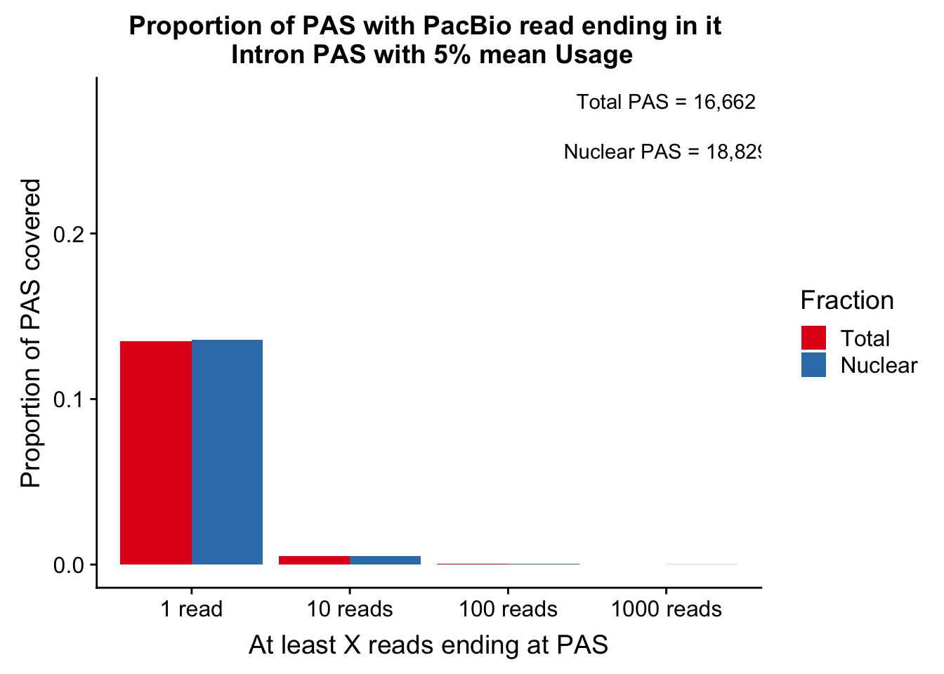
Do this for the UTR
UTRCov_tot5perc= utrCov %>% separate(ID, into=c("peak", "gene","loc"), sep=":") %>% semi_join(tot5Perc, by="peak")

UTRCov_nuc5perc= utrCov %>% separate(ID, into=c("peak", "gene","loc"), sep=":") %>% semi_join(nuc5Perc, by="peak")
utrCov_tot5perc_0= UTRCov_tot5perc %>% filter(cov> 0) %>% nrow()/ nrow(UTRCov_tot5perc)
utrCov_tot5perc_10= UTRCov_tot5perc %>% filter(cov>= 10) %>% nrow()/ nrow(UTRCov_tot5perc)
utrCov_tot5perc_100= UTRCov_tot5perc %>% filter(cov>= 100) %>% nrow()/ nrow(UTRCov_tot5perc)
utrCov_tot5perc_1000= UTRCov_tot5perc %>% filter(cov>= 1000) %>% nrow()/ nrow(UTRCov_tot5perc)
utrCov_nuc5perc_0= UTRCov_nuc5perc %>% filter(cov> 0) %>% nrow()/ nrow(UTRCov_nuc5perc)
utrCov_nuc5perc_10= UTRCov_nuc5perc %>% filter(cov>= 10) %>% nrow()/ nrow(UTRCov_nuc5perc)
utrCov_nuc5perc_100= UTRCov_nuc5perc %>% filter(cov>= 100) %>% nrow()/ nrow(UTRCov_nuc5perc)
utrCov_nuc5perc_1000= UTRCov_nuc5perc %>% filter(cov>= 1000) %>% nrow()/ nrow(UTRCov_nuc5perc)
Total_UTR=c(utrCov_tot5perc_0, utrCov_tot5perc_10, utrCov_tot5perc_100, utrCov_tot5perc_1000)
Nuclear_UTR=c(utrCov_nuc5perc_0,utrCov_nuc5perc_10,utrCov_nuc5perc_100,utrCov_nuc5perc_1000)
covUTR_5perDF=as.data.frame(cbind(Reads,Total=Total_UTR,Nuclear=Nuclear_UTR))
covUTR_5perDF$Total=as.numeric(as.character(covUTR_5perDF$Total))
covUTR_5perDF$Nuclear=as.numeric(as.character(covUTR_5perDF$Nuclear))
covUTR_5perDF_melt=melt(covUTR_5perDF, id.vars = "Reads")
colnames(covUTR_5perDF_melt)=c("ReadCutoff", "Fraction", "Proportion" )ggplot(covUTR_5perDF_melt, aes(x=ReadCutoff, fill=Fraction, y=Proportion, by=Fraction)) + geom_bar(position="dodge",stat="identity" ) + labs(y="Proportion of PAS covered", x="At least X reads ending at PAS", title="Proportion of PAS with PacBio read ending in it \n UTR PAS with 5% mean Usage") + scale_fill_brewer(palette = "Set1") + annotate("text", label="Total PAS = 5,984", x="1000 reads", y=.7) + annotate("text", label="Nuclear PAS = 6,793", x="1000 reads", y=.6)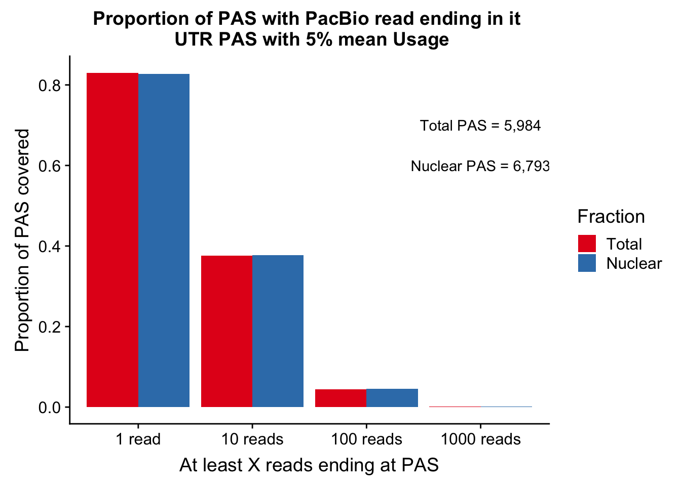
Make the first plot (utr v intron for the 5%) Process in excel
allProp=read.table("../data/pacbio_cov/PacBioPropCov.txt", head=T, stringsAsFactors = F)
allProp$Read=as.factor(allProp$Read)
allPropPlot=ggplot(allProp, aes(x=Read, y=Proportion, by=Location, fill=Location)) + geom_bar(position="dodge",stat="identity" ) +facet_grid(~Fraction) + labs(y="Proportion of PAS covered", x="At least X reads ending at PAS", title="Proportion of PAS with PacBio read ending in it \n PAS with 5% mean Usage")+scale_fill_manual(values=c("red","blue"))

allPropPlot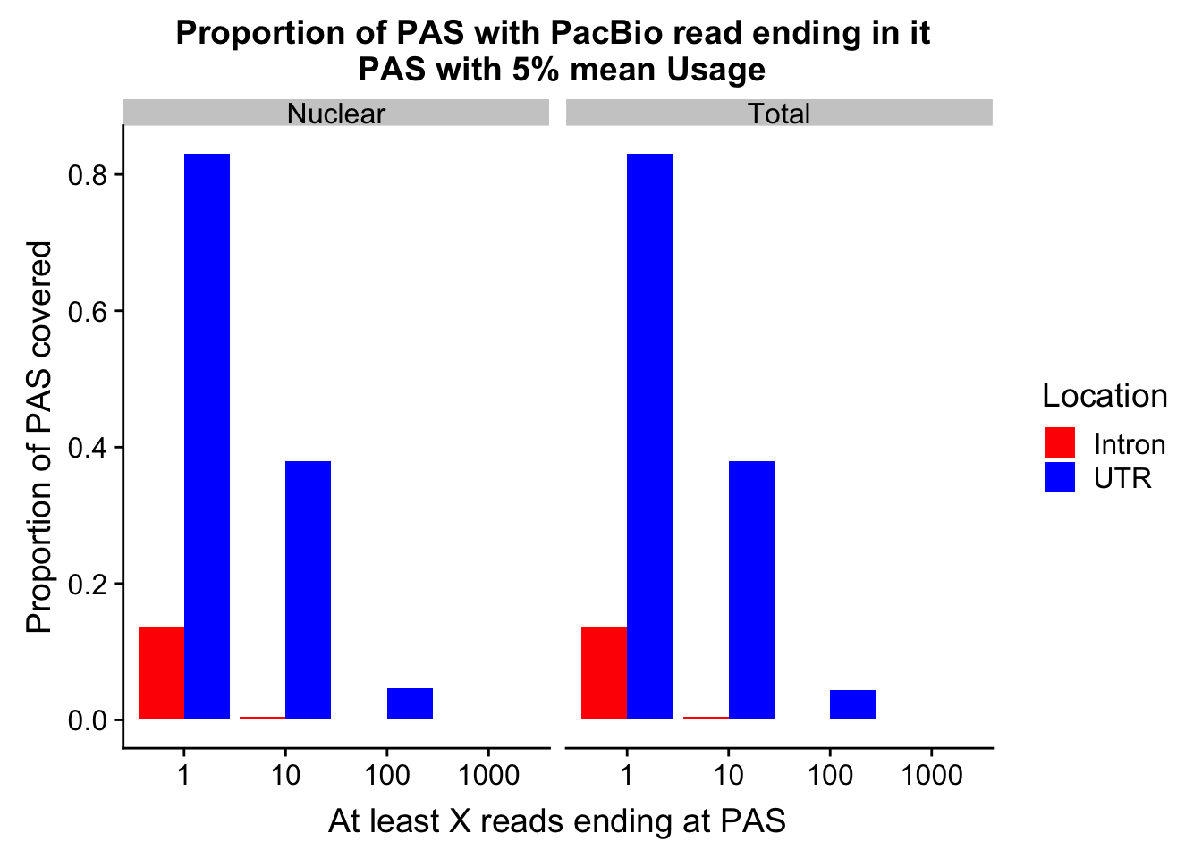
ggsave(allPropPlot, filename = "../output/plots/PacBioReadsEndingAtPAS_5percCov.png")Saving 7 x 5 in imageUTRCov_tot5perc %>% semi_join(UTRCov_nuc5perc, by="peak") %>% nrow()[1] 5538intronCov_tot5perc %>% semi_join(intronCov_nuc5perc, by="peak") %>% nrow()[1] 15270tot5Perc_peaks =tot5Perc %>% select(peak)
nuc5Perc_peaks=nuc5Perc %>% select(peak)
nrow(tot5Perc)[1] 33002nrow(nuc5Perc)[1] 37370ineither=tot5Perc_peaks %>% full_join(nuc5Perc_peaks, by="peak")
nrow(ineither)[1] 40066
sessionInfo()R version 3.5.1 (2018-07-02)
Platform: x86_64-apple-darwin15.6.0 (64-bit)
Running under: macOS 10.14.1
Matrix products: default
BLAS: /Library/Frameworks/R.framework/Versions/3.5/Resources/lib/libRblas.0.dylib
LAPACK: /Library/Frameworks/R.framework/Versions/3.5/Resources/lib/libRlapack.dylib
locale:
[1] en_US.UTF-8/en_US.UTF-8/en_US.UTF-8/C/en_US.UTF-8/en_US.UTF-8
attached base packages:
[1] stats graphics grDevices utils datasets methods base
other attached packages:
[1] bindrcpp_0.2.2 cowplot_0.9.3 reshape2_1.4.3 forcats_0.3.0
[5] stringr_1.4.0 dplyr_0.7.6 purrr_0.2.5 readr_1.1.1
[9] tidyr_0.8.1 tibble_1.4.2 ggplot2_3.0.0 tidyverse_1.2.1
[13] workflowr_1.2.0
loaded via a namespace (and not attached):
[1] tidyselect_0.2.4 haven_1.1.2 lattice_0.20-35
[4] colorspace_1.3-2 htmltools_0.3.6 yaml_2.2.0
[7] rlang_0.2.2 pillar_1.3.0 glue_1.3.0
[10] withr_2.1.2 RColorBrewer_1.1-2 modelr_0.1.2
[13] readxl_1.1.0 bindr_0.1.1 plyr_1.8.4
[16] munsell_0.5.0 gtable_0.2.0 cellranger_1.1.0
[19] rvest_0.3.2 evaluate_0.13 labeling_0.3
[22] knitr_1.20 broom_0.5.0 Rcpp_0.12.19
[25] scales_1.0.0 backports_1.1.2 jsonlite_1.6
[28] fs_1.2.6 hms_0.4.2 digest_0.6.17
[31] stringi_1.2.4 grid_3.5.1 rprojroot_1.3-2
[34] cli_1.0.1 tools_3.5.1 magrittr_1.5
[37] lazyeval_0.2.1 crayon_1.3.4 whisker_0.3-2
[40] pkgconfig_2.0.2 xml2_1.2.0 lubridate_1.7.4
[43] assertthat_0.2.0 rmarkdown_1.11 httr_1.3.1
[46] rstudioapi_0.9.0 R6_2.3.0 nlme_3.1-137
[49] git2r_0.24.0 compiler_3.5.1