39indQC
Briana Mittleman
2018-09-24
Last updated: 2018-09-25
workflowr checks: (Click a bullet for more information)-
✔ R Markdown file: up-to-date
Great! Since the R Markdown file has been committed to the Git repository, you know the exact version of the code that produced these results.
-
✔ Environment: empty
Great job! The global environment was empty. Objects defined in the global environment can affect the analysis in your R Markdown file in unknown ways. For reproduciblity it’s best to always run the code in an empty environment.
-
✔ Seed:
set.seed(12345)The command
set.seed(12345)was run prior to running the code in the R Markdown file. Setting a seed ensures that any results that rely on randomness, e.g. subsampling or permutations, are reproducible. -
✔ Session information: recorded
Great job! Recording the operating system, R version, and package versions is critical for reproducibility.
-
Great! You are using Git for version control. Tracking code development and connecting the code version to the results is critical for reproducibility. The version displayed above was the version of the Git repository at the time these results were generated.✔ Repository version: 66570c5
Note that you need to be careful to ensure that all relevant files for the analysis have been committed to Git prior to generating the results (you can usewflow_publishorwflow_git_commit). workflowr only checks the R Markdown file, but you know if there are other scripts or data files that it depends on. Below is the status of the Git repository when the results were generated:
Note that any generated files, e.g. HTML, png, CSS, etc., are not included in this status report because it is ok for generated content to have uncommitted changes.Ignored files: Ignored: .DS_Store Ignored: .Rhistory Ignored: .Rproj.user/ Ignored: output/.DS_Store Untracked files: Untracked: analysis/apaQTLsAllInd.Rmd Untracked: analysis/callMolQTLS.Rmd Untracked: analysis/ncbiRefSeq_sm.sort.mRNA.bed Untracked: analysis/snake.config.notes.Rmd Untracked: analysis/verifyBAM.Rmd Untracked: data/18486.genecov.txt Untracked: data/APApeaksYL.total.inbrain.bed Untracked: data/NuclearApaQTLs.txt Untracked: data/RNAkalisto/ Untracked: data/TotalApaQTLs.txt Untracked: data/Totalpeaks_filtered_clean.bed Untracked: data/YL-SP-18486-T-combined-genecov.txt Untracked: data/YL-SP-18486-T_S9_R1_001-genecov.txt Untracked: data/bedgraph_peaks/ Untracked: data/bin200.5.T.nuccov.bed Untracked: data/bin200.Anuccov.bed Untracked: data/bin200.nuccov.bed Untracked: data/clean_peaks/ Untracked: data/comb_map_stats.csv Untracked: data/comb_map_stats.xlsx Untracked: data/comb_map_stats_39ind.csv Untracked: data/combined_reads_mapped_three_prime_seq.csv Untracked: data/gencov.test.csv Untracked: data/gencov.test.txt Untracked: data/gencov_zero.test.csv Untracked: data/gencov_zero.test.txt Untracked: data/gene_cov/ Untracked: data/joined Untracked: data/leafcutter/ Untracked: data/merged_combined_YL-SP-threeprimeseq.bg Untracked: data/nom_QTL/ Untracked: data/nom_QTL_opp/ Untracked: data/nuc6up/ Untracked: data/other_qtls/ Untracked: data/peakPerRefSeqGene/ Untracked: data/perm_QTL/ Untracked: data/perm_QTL_opp/ Untracked: data/reads_mapped_three_prime_seq.csv Untracked: data/smash.cov.results.bed Untracked: data/smash.cov.results.csv Untracked: data/smash.cov.results.txt Untracked: data/smash_testregion/ Untracked: data/ssFC200.cov.bed Untracked: data/temp.file1 Untracked: data/temp.file2 Untracked: data/temp.gencov.test.txt Untracked: data/temp.gencov_zero.test.txt Untracked: output/picard/ Untracked: output/plots/ Untracked: output/qual.fig2.pdf Unstaged changes: Modified: analysis/28ind.peak.explore.Rmd Modified: analysis/cleanupdtseq.internalpriming.Rmd Modified: analysis/dif.iso.usage.leafcutter.Rmd Modified: analysis/diff_iso_pipeline.Rmd Modified: analysis/explore.filters.Rmd Modified: analysis/overlap_qtls.Rmd Modified: analysis/peakOverlap_oppstrand.Rmd Modified: analysis/pheno.leaf.comb.Rmd Modified: analysis/test.max2.Rmd Modified: code/Snakefile
Expand here to see past versions:
I will use this to look at the map stats and peak stats for the full set of 39 ind.
library(tidyverse)── Attaching packages ──────────────────────────────────────────────────────────────────────────────────────────── tidyverse 1.2.1 ──✔ ggplot2 3.0.0 ✔ purrr 0.2.5
✔ tibble 1.4.2 ✔ dplyr 0.7.6
✔ tidyr 0.8.1 ✔ stringr 1.3.1
✔ readr 1.1.1 ✔ forcats 0.3.0── Conflicts ─────────────────────────────────────────────────────────────────────────────────────────────── tidyverse_conflicts() ──
✖ dplyr::filter() masks stats::filter()
✖ dplyr::lag() masks stats::lag()library(workflowr)This is workflowr version 1.1.1
Run ?workflowr for help getting startedlibrary(reshape2)
Attaching package: 'reshape2'The following object is masked from 'package:tidyr':
smithslibrary(cowplot)
Attaching package: 'cowplot'The following object is masked from 'package:ggplot2':
ggsavelibrary(tximport)Map Stats
mapstats= read.csv("../data/comb_map_stats_39ind.csv", header = T, stringsAsFactors = F)
mapstats$line=as.factor(mapstats$line)
mapstats$fraction=as.factor(mapstats$fraction)
map_melt=melt(mapstats, id.vars=c("line", "fraction"), measure.vars = c("comb_reads", "comb_mapped", "comb_prop_mapped"))

prop_mapped= map_melt %>% filter(variable=="comb_prop_mapped")
mapped_reads= map_melt %>% filter(variable=="comb_mapped")


mapplot_prop=ggplot(prop_mapped, aes(y=value, x=line, fill=fraction)) + geom_bar(stat="identity",position="dodge") + labs( title="Proportion of reads mapped") + ylab("Proportion mapped")


mapplot_mapped=ggplot(mapped_reads, aes(y=value, x=line, fill=fraction)) + geom_bar(stat="identity",position="dodge") + labs( title="Number of Mapped reads") + ylab("Mapped")

plot_grid(mapplot_prop, mapplot_mapped)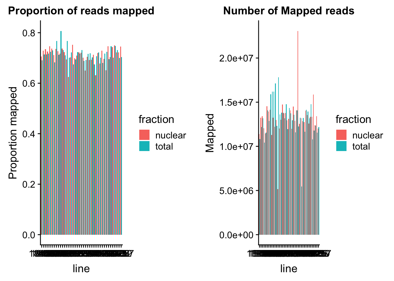
Expand here to see past versions of unnamed-chunk-2-1.png:
| Version | Author | Date |
|---|---|---|
| d3bb287 | Briana Mittleman | 2018-09-24 |
Plot boxplots for total vs nuclear.
box_mapprop=ggplot(prop_mapped, aes(y=value, x=fraction, fill=fraction)) + geom_boxplot() + geom_jitter(position = position_jitter(.3)) + labs( title="Map Proportion") + ylab("Mapped Proportion")

box_map=ggplot(mapped_reads, aes(y=value, x=fraction, fill=fraction)) + geom_boxplot() + geom_jitter(position = position_jitter(.3)) + labs( title="Number of Mapped reads") + ylab("Mapped")


plot_grid(box_map, box_mapprop)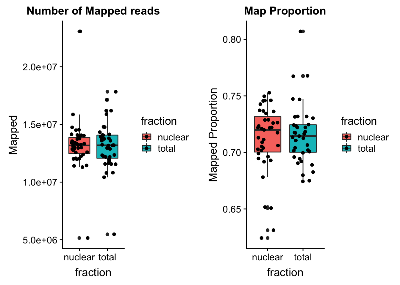
Expand here to see past versions of unnamed-chunk-3-1.png:
| Version | Author | Date |
|---|---|---|
| d3bb287 | Briana Mittleman | 2018-09-24 |
Genes with multiple peaks
This is similar to the analysis I ran in dataprocfigures.Rmd. I start by overlappping the refseq genes with my peaks. With the script refseq_countdistinct.sh.
namesPeak=c("Chr", "Start", "End", "Name", "Score", "Strand", "numPeaks")
Opeakpergene=read.table("../data/peakPerRefSeqGene/filtered_APApeaks_perRefseqGene_oppStrand.txt", stringsAsFactors = F, header = F, col.names = namesPeak) %>% mutate(onePeak=ifelse(numPeaks==1, 1, 0 )) %>%  mutate(multPeaks=ifelse(numPeaks > 1, 1, 0 ))

Ogenes1peak=sum(Opeakpergene$onePeak)/nrow(Opeakpergene)
OgenesMultpeak=sum(Opeakpergene$multPeaks)/nrow(Opeakpergene)
Ogenes0peak= 1- Ogenes1peak - OgenesMultpeak


OperPeak= c(round(Ogenes0peak,digits = 3), round(Ogenes1peak,digits = 3),round(OgenesMultpeak, digits = 3))
Category=c("Zero", "One", "Multiple")
OperPeakdf=as.data.frame(cbind(Category,OperPeak))

OperPeakdf$OperPeak=as.numeric(as.character(OperPeakdf$OperPeak))

Olab1=paste("Genes =", Ogenes0peak*nrow(Opeakpergene), sep=" ")
Olab2=paste("Genes =", sum(Opeakpergene$onePeak), sep=" ")
Olab3=paste("Genes =", sum(Opeakpergene$multPeaks), sep=" ")

Ogenepeakplot=ggplot(OperPeakdf, aes(x="", y=OperPeak, by=Category, fill=Category)) + geom_bar(stat="identity")+ labs(title="Characterize Refseq genes by number of PAS- Oppstrand", y="Proportion of Protein Coding gene", x="")+ scale_fill_brewer(palette="Paired") + coord_cartesian(ylim=c(0,1)) + annotate("text", x="", y= .2, label=Olab1) + annotate("text", x="", y= .4, label=Olab2) + annotate("text", x="", y= .9, label=Olab3)
Ogenepeakplot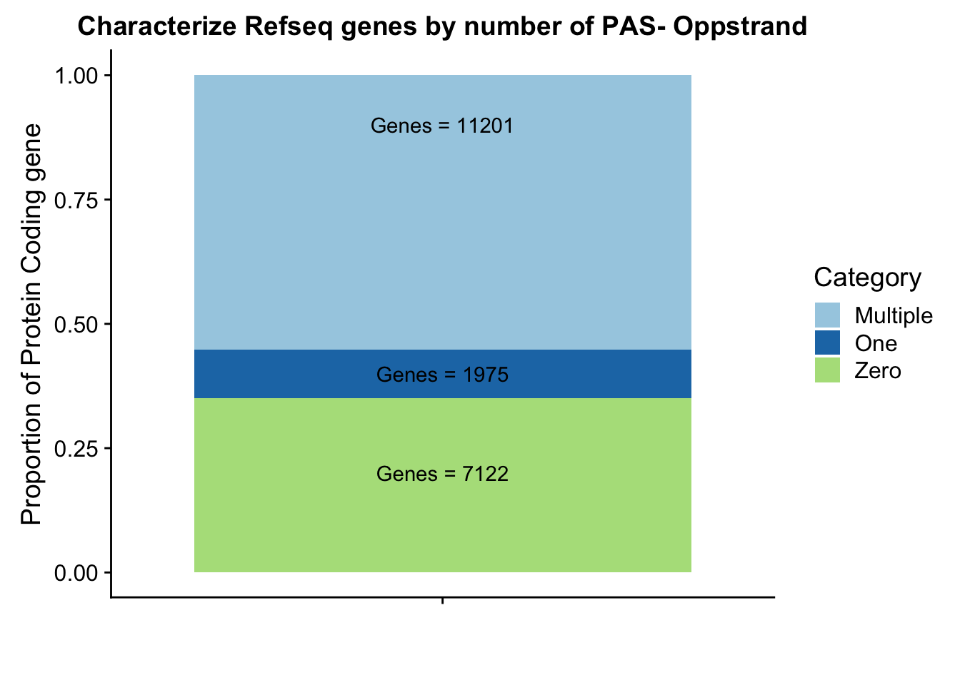
I will now repull in the RNA seq data for one of my lines to look at the expression levels of the genes with at least 1 called peak.
tx2gene=read.table("../data/RNAkalisto/ncbiRefSeq.txn2gene.txt" ,header= F, sep="\t", stringsAsFactors = F)

txi.kallisto.tsv <- tximport("../data/RNAkalisto/abundance.tsv", type = "kallisto", tx2gene = tx2gene)
Note: importing `abundance.h5` is typically faster than `abundance.tsv`reading in files with read_tsv1
removing duplicated transcript rows from tx2gene
transcripts missing from tx2gene: 99
summarizing abundance
summarizing counts
summarizing lengthtxi.kallisto.tsv$abundance= as.data.frame(txi.kallisto.tsv$abundance) %>% rownames_to_column(var="Name")
colnames(txi.kallisto.tsv$abundance)= c("Name", "TPM")
#genes with >0 TPM and at least 1 peak
refPeakandRNA_withO_TPM=Opeakpergene %>% inner_join(txi.kallisto.tsv$abundance, by="Name") %>% filter(TPM>0, numPeaks>0)
#genes with >0 TPM and 0 peak
refPeakandRNA_noPeakw_withO_TPM=Opeakpergene %>% inner_join(txi.kallisto.tsv$abundance, by="Name") %>% filter(TPM >0, numPeaks==0)
#plot
plot(sort(log10(refPeakandRNA_withO_TPM$TPM), decreasing = T), main="Distribution of RNA expression 18486", ylab="log10 TPM", xlab="Refseq Gene")
points(sort(log10(refPeakandRNA_noPeakw_withO_TPM$TPM), decreasing = T), col="Red")
legend("topright", legend=c("Genes wth Peak", "Genes without Peak"), col=c("black", "red"),pch=19)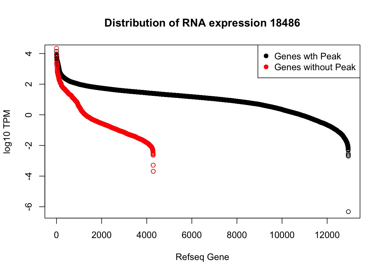
Plot this as distributions.
comp_RNAtpm=ggplot(refPeakandRNA_withO_TPM, aes(x=log10(TPM))) + geom_histogram(binwidth=.5, alpha=.5) +geom_histogram(data = refPeakandRNA_noPeakw_withO_TPM, aes(x=log10(TPM)), fill="Red", alpha=.5, binwidth=.5) + labs(title="Comparing RNA expression for genes with a PAS vs no PAS") + annotate("text", x=-8, y=3000, col="Red", label="Genes without PAS") + annotate("text", x=-8.1, y=2700, col="Black", label="Genes with PAS") + geom_rect(linetype=1, xmin=-10, xmax=-6, ymin=2500, ymax=3200, color="Black", alpha=0)
comp_RNAtpm
Session information
sessionInfo()R version 3.5.1 (2018-07-02)
Platform: x86_64-apple-darwin15.6.0 (64-bit)
Running under: macOS Sierra 10.12.6
Matrix products: default
BLAS: /Library/Frameworks/R.framework/Versions/3.5/Resources/lib/libRblas.0.dylib
LAPACK: /Library/Frameworks/R.framework/Versions/3.5/Resources/lib/libRlapack.dylib
locale:
[1] en_US.UTF-8/en_US.UTF-8/en_US.UTF-8/C/en_US.UTF-8/en_US.UTF-8
attached base packages:
[1] stats graphics grDevices utils datasets methods base
other attached packages:
[1] bindrcpp_0.2.2 tximport_1.8.0 cowplot_0.9.3 reshape2_1.4.3
[5] workflowr_1.1.1 forcats_0.3.0 stringr_1.3.1 dplyr_0.7.6
[9] purrr_0.2.5 readr_1.1.1 tidyr_0.8.1 tibble_1.4.2
[13] ggplot2_3.0.0 tidyverse_1.2.1
loaded via a namespace (and not attached):
[1] tidyselect_0.2.4 haven_1.1.2 lattice_0.20-35
[4] colorspace_1.3-2 htmltools_0.3.6 yaml_2.2.0
[7] rlang_0.2.2 R.oo_1.22.0 pillar_1.3.0
[10] glue_1.3.0 withr_2.1.2 R.utils_2.7.0
[13] RColorBrewer_1.1-2 modelr_0.1.2 readxl_1.1.0
[16] bindr_0.1.1 plyr_1.8.4 munsell_0.5.0
[19] gtable_0.2.0 cellranger_1.1.0 rvest_0.3.2
[22] R.methodsS3_1.7.1 evaluate_0.11 labeling_0.3
[25] knitr_1.20 broom_0.5.0 Rcpp_0.12.18
[28] scales_1.0.0 backports_1.1.2 jsonlite_1.5
[31] hms_0.4.2 digest_0.6.16 stringi_1.2.4
[34] grid_3.5.1 rprojroot_1.3-2 cli_1.0.0
[37] tools_3.5.1 magrittr_1.5 lazyeval_0.2.1
[40] crayon_1.3.4 whisker_0.3-2 pkgconfig_2.0.2
[43] xml2_1.2.0 lubridate_1.7.4 assertthat_0.2.0
[46] rmarkdown_1.10 httr_1.3.1 rstudioapi_0.7
[49] R6_2.2.2 nlme_3.1-137 git2r_0.23.0
[52] compiler_3.5.1
This reproducible R Markdown analysis was created with workflowr 1.1.1