Coverage analysis
Briana Mittleman
7/13/2018
Last updated: 2018-07-13
workflowr checks: (Click a bullet for more information)-
✔ R Markdown file: up-to-date
Great! Since the R Markdown file has been committed to the Git repository, you know the exact version of the code that produced these results.
-
✔ Environment: empty
Great job! The global environment was empty. Objects defined in the global environment can affect the analysis in your R Markdown file in unknown ways. For reproduciblity it’s best to always run the code in an empty environment.
-
✔ Seed:
set.seed(12345)The command
set.seed(12345)was run prior to running the code in the R Markdown file. Setting a seed ensures that any results that rely on randomness, e.g. subsampling or permutations, are reproducible. -
✔ Session information: recorded
Great job! Recording the operating system, R version, and package versions is critical for reproducibility.
-
Great! You are using Git for version control. Tracking code development and connecting the code version to the results is critical for reproducibility. The version displayed above was the version of the Git repository at the time these results were generated.✔ Repository version: 4a84769
Note that you need to be careful to ensure that all relevant files for the analysis have been committed to Git prior to generating the results (you can usewflow_publishorwflow_git_commit). workflowr only checks the R Markdown file, but you know if there are other scripts or data files that it depends on. Below is the status of the Git repository when the results were generated:
Note that any generated files, e.g. HTML, png, CSS, etc., are not included in this status report because it is ok for generated content to have uncommitted changes.Ignored files: Ignored: .DS_Store Ignored: .Rhistory Ignored: .Rproj.user/ Ignored: output/.DS_Store Untracked files: Untracked: data/18486.genecov.txt Untracked: data/YL-SP-18486-T_S9_R1_001-genecov.txt Untracked: data/bedgraph_peaks/ Untracked: data/bin200.5.T.nuccov.bed Untracked: data/bin200.Anuccov.bed Untracked: data/bin200.nuccov.bed Untracked: data/gene_cov/ Untracked: data/leafcutter/ Untracked: data/nuc6up/ Untracked: data/reads_mapped_three_prime_seq.csv Untracked: data/ssFC200.cov.bed Untracked: output/picard/ Untracked: output/plots/ Untracked: output/qual.fig2.pdf Unstaged changes: Modified: analysis/dif.iso.usage.leafcutter.Rmd Modified: analysis/explore.filters.Rmd Modified: analysis/test.max2.Rmd Modified: code/Snakefile
Expand here to see past versions:
| File | Version | Author | Date | Message |
|---|---|---|---|---|
| Rmd | 4a84769 | Briana Mittleman | 2018-07-13 | add analysis for coparing coverage of RNAseq and 3’ seq |
I will use this analysis to compare the 3’ seq data to the RNA seq data. I am going to look at the protein coding genes.
library(workflowr)Loading required package: rmarkdownThis is workflowr version 1.0.1
Run ?workflowr for help getting startedlibrary(ggplot2)
library(tidyr)
library(dplyr)Warning: package 'dplyr' was built under R version 3.4.4
Attaching package: 'dplyr'The following objects are masked from 'package:stats':
filter, lagThe following objects are masked from 'package:base':
intersect, setdiff, setequal, unionlibrary(reshape2)Warning: package 'reshape2' was built under R version 3.4.3
Attaching package: 'reshape2'The following object is masked from 'package:tidyr':
smithsLoad RNA seq gene cov for 18486.
rnaseq=read.table("../data/18486.genecov.txt")
names(rnaseq)=c("Chr", "start", "end", "gene", "score", "strand", "count")
rnaseq_counts= rnaseq %>% select(gene, count)
Load all total fraction 3’ seq libraries.
t18486=read.table("../data/gene_cov/YL-SP-18486-T_S9_R1_001-genecov.txt",col.names =c("Chr", "start", "end", "gene", "score", "strand", "T18486") )
t18497=read.table("../data/gene_cov/YL-SP-18497-T_S11_R1_001-genecov.txt",col.names =c("Chr", "start", "end", "gene", "score", "strand", "T18497") )
t18500=read.table("../data/gene_cov/YL-SP-18500-T_S19_R1_001-genecov.txt",col.names =c("Chr", "start", "end", "gene", "score", "strand", "T18500") )
t18505=read.table("../data/gene_cov/YL-SP-18500-T_S19_R1_001-genecov.txt",col.names =c("Chr", "start", "end", "gene", "score", "strand", "T18505") )
t18508=read.table("../data/gene_cov/YL-SP-18508-T_S5_R1_001-genecov.txt",col.names =c("Chr", "start", "end", "gene", "score", "strand", "T18508") )
t18853=read.table("../data/gene_cov/YL-SP-18853-T_S31_R1_001-genecov.txt",col.names =c("Chr", "start", "end", "gene", "score", "strand", "T18853") )
t18870=read.table("../data/gene_cov/YL-SP-18870-T_S23_R1_001-genecov.txt",col.names =c("Chr", "start", "end", "gene", "score", "strand", "T18870") )
t19128=read.table("../data/gene_cov/YL-SP-19128-T_S29_R1_001-genecov.txt",col.names =c("Chr", "start", "end", "gene", "score", "strand", "T19128") )
t19141=read.table("../data/gene_cov/YL-SP-19141-T_S17_R1_001-genecov.txt",col.names =c("Chr", "start", "end", "gene", "score", "strand", "T19141") )
t19193=read.table("../data/gene_cov/YL-SP-19193-T_S21_R1_001-genecov.txt",col.names =c("Chr", "start", "end", "gene", "score", "strand", "T19193") )
t19209=read.table("../data/gene_cov/YL-SP-19209-T_S15_R1_001-genecov.txt",col.names =c("Chr", "start", "end", "gene", "score", "strand", "T19209") )
t19223=read.table("../data/gene_cov/YL-SP-19233-T_S7_R1_001-genecov.txt",col.names =c("Chr", "start", "end", "gene", "score", "strand", "T19223") )
t19225=read.table("../data/gene_cov/YL-SP-19225-T_S27_R1_001-genecov.txt",col.names =c("Chr", "start", "end", "gene", "score", "strand", "T19225") )
t19238=read.table("../data/gene_cov/YL-SP-19238-T_S3_R1_001-genecov.txt",col.names =c("Chr", "start", "end", "gene", "score", "strand", "T19238") )
t19239=read.table("../data/gene_cov/YL-SP-19239-T_S13_R1_001-genecov.txt",col.names =c("Chr", "start", "end", "gene", "score", "strand", "T19239") )
t19257=read.table("../data/gene_cov/YL-SP-19257-T_S25_R1_001-genecov.txt",col.names =c("Chr", "start", "end", "gene", "score", "strand", "T19257") )
Merge all of the files:
threeprimeall=cbind(t18486,t18497$T18497, t18500$T18500, t18505$T18505, t18508$T18508, t18853$T18853, t18870$T18870, t19128$T19128, t19141$T19141,t19193$T19193, t19209$T19209, t19223$T19223, t19225$T19225, t19238$T19238, t19239$T19239, t19257$T19257)


threeprimeall_sum=threeprimeall %>% mutate(Counts_all= T18486,t18497$T18497, t18500$T18500, t18505$T18505, t18508$T18508, t18853$T18853, t18870$T18870, t19128$T19128, t19141$T19141,t19193$T19193, t19209$T19209, t19223$T19223, t19225$T19225, t19238$T19238, t19239$T19239, t19257$T19257) %>% select(gene, Counts_all)
Warning: package 'bindrcpp' was built under R version 3.4.4threeprimeall_sum$gene=as.character(threeprimeall_sum$gene)Melt the data fro ggplot.
all_counts= cbind(threeprimeall_sum,rnaseq_counts$count)
colnames(all_counts)= c("gene", "threeprime", "RNAseq")

all_counts_melt= melt(all_counts, id.vars="gene")
names(all_counts_melt)=c("gene", "Library", "Count")
Plot the CDFs
ggplot(all_counts_melt, aes(x=log10(Count), col=Library)) + stat_ecdf(geom = "step", pad = FALSE) + labs(title= "Log10 counts CDF")Warning: Removed 9859 rows containing non-finite values (stat_ecdf).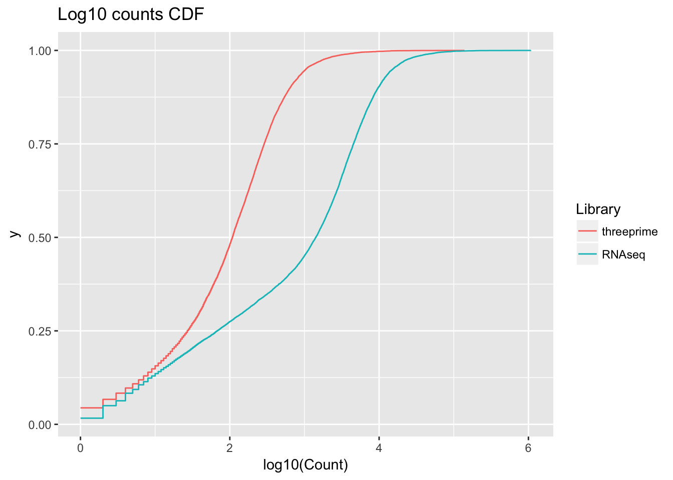
Session information
sessionInfo()R version 3.4.2 (2017-09-28)
Platform: x86_64-apple-darwin15.6.0 (64-bit)
Running under: macOS Sierra 10.12.6
Matrix products: default
BLAS: /Library/Frameworks/R.framework/Versions/3.4/Resources/lib/libRblas.0.dylib
LAPACK: /Library/Frameworks/R.framework/Versions/3.4/Resources/lib/libRlapack.dylib
locale:
[1] en_US.UTF-8/en_US.UTF-8/en_US.UTF-8/C/en_US.UTF-8/en_US.UTF-8
attached base packages:
[1] stats graphics grDevices utils datasets methods base
other attached packages:
[1] bindrcpp_0.2.2 reshape2_1.4.3 dplyr_0.7.5 tidyr_0.7.2
[5] ggplot2_2.2.1 workflowr_1.0.1 rmarkdown_1.8.5
loaded via a namespace (and not attached):
[1] Rcpp_0.12.17 compiler_3.4.2 pillar_1.1.0
[4] git2r_0.21.0 plyr_1.8.4 bindr_0.1.1
[7] R.methodsS3_1.7.1 R.utils_2.6.0 tools_3.4.2
[10] digest_0.6.15 evaluate_0.10.1 tibble_1.4.2
[13] gtable_0.2.0 pkgconfig_2.0.1 rlang_0.2.1
[16] yaml_2.1.19 stringr_1.3.1 knitr_1.18
[19] rprojroot_1.3-2 grid_3.4.2 tidyselect_0.2.4
[22] glue_1.2.0 R6_2.2.2 purrr_0.2.5
[25] magrittr_1.5 whisker_0.3-2 backports_1.1.2
[28] scales_0.5.0 htmltools_0.3.6 assertthat_0.2.0
[31] colorspace_1.3-2 labeling_0.3 stringi_1.2.2
[34] lazyeval_0.2.1 munsell_0.4.3 R.oo_1.22.0
This reproducible R Markdown analysis was created with workflowr 1.0.1