Understand Peaks

Last updated: 2018-12-05

workflowr checks: (Click a bullet for more information)

✔ R Markdown file: up-to-date

Great! Since the R Markdown file has been committed to the Git repository, you know the exact version of the code that produced these results.
✔ Environment: empty

Great job! The global environment was empty. Objects defined in the global environment can affect the analysis in your R Markdown file in unknown ways. For reproduciblity it’s best to always run the code in an empty environment.
✔ Seed: set.seed(12345)

The command set.seed(12345) was run prior to running the code in the R Markdown file. Setting a seed ensures that any results that rely on randomness, e.g. subsampling or permutations, are reproducible.
✔ Session information: recorded

Great job! Recording the operating system, R version, and package versions is critical for reproducibility.

✔ Repository version: 655b582

Great! You are using Git for version control. Tracking code development and connecting the code version to the results is critical for reproducibility. The version displayed above was the version of the Git repository at the time these results were generated.

Note that you need to be careful to ensure that all relevant files for the analysis have been committed to Git prior to generating the results (you can use wflow_publish or wflow_git_commit). workflowr only checks the R Markdown file, but you know if there are other scripts or data files that it depends on. Below is the status of the Git repository when the results were generated:


Ignored files:
    Ignored:    .DS_Store
    Ignored:    .Rhistory
    Ignored:    .Rproj.user/
    Ignored:    data/.DS_Store
    Ignored:    output/.DS_Store

Untracked files:
    Untracked:  KalistoAbundance18486.txt
    Untracked:  analysis/DirectionapaQTL.Rmd
    Untracked:  analysis/ncbiRefSeq_sm.sort.mRNA.bed
    Untracked:  analysis/snake.config.notes.Rmd
    Untracked:  analysis/verifyBAM.Rmd
    Untracked:  data/18486.genecov.txt
    Untracked:  data/APApeaksYL.total.inbrain.bed
    Untracked:  data/ChromHmmOverlap/
    Untracked:  data/GM12878.chromHMM.bed
    Untracked:  data/GM12878.chromHMM.txt
    Untracked:  data/LocusZoom/
    Untracked:  data/NuclearApaQTLs.txt
    Untracked:  data/PeakCounts/
    Untracked:  data/PeaksUsed/
    Untracked:  data/RNAkalisto/
    Untracked:  data/TotalApaQTLs.txt
    Untracked:  data/Totalpeaks_filtered_clean.bed
    Untracked:  data/YL-SP-18486-T-combined-genecov.txt
    Untracked:  data/YL-SP-18486-T_S9_R1_001-genecov.txt
    Untracked:  data/apaExamp/
    Untracked:  data/bedgraph_peaks/
    Untracked:  data/bin200.5.T.nuccov.bed
    Untracked:  data/bin200.Anuccov.bed
    Untracked:  data/bin200.nuccov.bed
    Untracked:  data/clean_peaks/
    Untracked:  data/comb_map_stats.csv
    Untracked:  data/comb_map_stats.xlsx
    Untracked:  data/comb_map_stats_39ind.csv
    Untracked:  data/combined_reads_mapped_three_prime_seq.csv
    Untracked:  data/diff_iso_trans/
    Untracked:  data/ensemble_to_genename.txt
    Untracked:  data/example_gene_peakQuant/
    Untracked:  data/explainProtVar/
    Untracked:  data/filtered_APApeaks_merged_allchrom_refseqTrans.closest2End.bed
    Untracked:  data/filtered_APApeaks_merged_allchrom_refseqTrans.closest2End.noties.bed
    Untracked:  data/first50lines_closest.txt
    Untracked:  data/gencov.test.csv
    Untracked:  data/gencov.test.txt
    Untracked:  data/gencov_zero.test.csv
    Untracked:  data/gencov_zero.test.txt
    Untracked:  data/gene_cov/
    Untracked:  data/joined
    Untracked:  data/leafcutter/
    Untracked:  data/merged_combined_YL-SP-threeprimeseq.bg
    Untracked:  data/mol_overlap/
    Untracked:  data/mol_pheno/
    Untracked:  data/nom_QTL/
    Untracked:  data/nom_QTL_opp/
    Untracked:  data/nom_QTL_trans/
    Untracked:  data/nuc6up/
    Untracked:  data/other_qtls/
    Untracked:  data/pQTL_otherphen/
    Untracked:  data/peakPerRefSeqGene/
    Untracked:  data/perm_QTL/
    Untracked:  data/perm_QTL_opp/
    Untracked:  data/perm_QTL_trans/
    Untracked:  data/perm_QTL_trans_filt/
    Untracked:  data/reads_mapped_three_prime_seq.csv
    Untracked:  data/smash.cov.results.bed
    Untracked:  data/smash.cov.results.csv
    Untracked:  data/smash.cov.results.txt
    Untracked:  data/smash_testregion/
    Untracked:  data/ssFC200.cov.bed
    Untracked:  data/temp.file1
    Untracked:  data/temp.file2
    Untracked:  data/temp.gencov.test.txt
    Untracked:  data/temp.gencov_zero.test.txt
    Untracked:  output/picard/
    Untracked:  output/plots/
    Untracked:  output/qual.fig2.pdf

Unstaged changes:
    Modified:   analysis/28ind.peak.explore.Rmd
    Modified:   analysis/apaQTLoverlapGWAS.Rmd
    Modified:   analysis/cleanupdtseq.internalpriming.Rmd
    Modified:   analysis/coloc_apaQTLs_protQTLs.Rmd
    Modified:   analysis/dif.iso.usage.leafcutter.Rmd
    Modified:   analysis/diff_iso_pipeline.Rmd
    Modified:   analysis/explainpQTLs.Rmd
    Modified:   analysis/explore.filters.Rmd
    Modified:   analysis/flash2mash.Rmd
    Modified:   analysis/overlapMolQTL.Rmd
    Modified:   analysis/overlap_qtls.Rmd
    Modified:   analysis/peakOverlap_oppstrand.Rmd
    Modified:   analysis/pheno.leaf.comb.Rmd
    Modified:   analysis/swarmPlots_QTLs.Rmd
    Modified:   analysis/test.max2.Rmd
    Modified:   code/Snakefile

Note that any generated files, e.g. HTML, png, CSS, etc., are not included in this status report because it is ok for generated content to have uncommitted changes.

Expand here to see past versions:

File	Version	Author	Date	Message
Rmd	655b582	Briana Mittleman	2018-12-05	PCA with batch and read count

The goal of this analysis is to understand the data a bit better at the peak level. I want to have the cleanest set of peaks when I perform the final anlyses for the paper.

Variation in peaks

First I will run PCA on the peak coverage. I will run this seperatly for the total and nuclear fractions. I do not expect large amount of separation.

I will use the peak coverage data before the ratios are created for leafcutter. These files were created using feature counts on the filtered peaks. At this point the peaks have been mapped to the closest refseq transcript on the opposite strand.

Relevant file:
* /project2/gilad/briana/threeprimeseq/data/filtPeakOppstrand_cov/filtered_APApeaks_merged_allchrom_refseqGenes.Transcript_sm_quant.Total_fixed.fc

/project2/gilad/briana/threeprimeseq/data/filtPeakOppstrand_cov/filtered_APApeaks_merged_allchrom_refseqGenes.Transcript_sm_quant.Nuclear_fixed.fc

These files are in /Users/bmittleman1/Documents/Gilad_lab/threeprimeseq/data/PeakCounts on my computer.

library(tidyverse)

── Attaching packages ───────────────────────────────────────────────────────── tidyverse 1.2.1 ──

✔ ggplot2 3.0.0     ✔ purrr   0.2.5
✔ tibble  1.4.2     ✔ dplyr   0.7.6
✔ tidyr   0.8.1     ✔ stringr 1.3.1
✔ readr   1.1.1     ✔ forcats 0.3.0

── Conflicts ──────────────────────────────────────────────────────────── tidyverse_conflicts() ──
✖ dplyr::filter() masks stats::filter()
✖ dplyr::lag()    masks stats::lag()

library(workflowr)

This is workflowr version 1.1.1
Run ?workflowr for help getting started

library(cowplot)


Attaching package: 'cowplot'

The following object is masked from 'package:ggplot2':

    ggsave

library(reshape2)


Attaching package: 'reshape2'

The following object is masked from 'package:tidyr':

    smiths

library(devtools)

Load data:

#only keep the counts 
total_Cov=read.table("../data/PeakCounts/filtered_APApeaks_merged_allchrom_refseqGenes.Transcript_sm_quant.Total_fixed.fc", header=T, stringsAsFactors = F)[,7:45]
nuclear_Cov=read.table("../data/PeakCounts/filtered_APApeaks_merged_allchrom_refseqGenes.Transcript_sm_quant.Nuclear_fixed.fc", header=T, stringsAsFactors = F)[,7:45]

Total:

Run PCA on the total coverage

pca_tot_peak=prcomp(total_Cov, center=T,scale=T)
summary(pca_tot_peak)

Importance of components:
                          PC1     PC2     PC3     PC4     PC5    PC6
Standard deviation     5.9010 1.30000 0.81376 0.75658 0.47993 0.4501
Proportion of Variance 0.8929 0.04333 0.01698 0.01468 0.00591 0.0052
Cumulative Proportion  0.8929 0.93621 0.95319 0.96787 0.97378 0.9790
                           PC7     PC8     PC9    PC10    PC11    PC12
Standard deviation     0.42896 0.32313 0.30419 0.27984 0.23427 0.19916
Proportion of Variance 0.00472 0.00268 0.00237 0.00201 0.00141 0.00102
Cumulative Proportion  0.98369 0.98637 0.98874 0.99075 0.99216 0.99317
                          PC13    PC14    PC15    PC16    PC17   PC18
Standard deviation     0.18883 0.15913 0.15127 0.14309 0.12758 0.1254
Proportion of Variance 0.00091 0.00065 0.00059 0.00053 0.00042 0.0004
Cumulative Proportion  0.99409 0.99474 0.99532 0.99585 0.99626 0.9967
                          PC19    PC20    PC21    PC22    PC23    PC24
Standard deviation     0.12328 0.11035 0.10707 0.09979 0.09530 0.08797
Proportion of Variance 0.00039 0.00031 0.00029 0.00026 0.00023 0.00020
Cumulative Proportion  0.99706 0.99737 0.99766 0.99792 0.99815 0.99835
                          PC25    PC26    PC27    PC28    PC29    PC30
Standard deviation     0.08576 0.08086 0.07902 0.07535 0.07454 0.06907
Proportion of Variance 0.00019 0.00017 0.00016 0.00015 0.00014 0.00012
Cumulative Proportion  0.99854 0.99871 0.99887 0.99901 0.99916 0.99928
                          PC31    PC32    PC33    PC34    PC35    PC36
Standard deviation     0.06717 0.06441 0.06201 0.05666 0.05415 0.05261
Proportion of Variance 0.00012 0.00011 0.00010 0.00008 0.00008 0.00007
Cumulative Proportion  0.99939 0.99950 0.99960 0.99968 0.99976 0.99983
                          PC37    PC38    PC39
Standard deviation     0.05128 0.04839 0.04237
Proportion of Variance 0.00007 0.00006 0.00005
Cumulative Proportion  0.99989 0.99995 1.00000

pca_tot_df=as.data.frame(pca_tot_peak$rotation) %>% rownames_to_column(var="lib") %>% mutate(line=substr(lib,2,6))
pca_tot_df$line=as.integer(pca_tot_df$line)

I want to color these by library size.

map_stats=read.csv("../data/comb_map_stats_39ind.csv", header=T)

map_stat_total=map_stats %>% filter(fraction=="total")
map_stat_total$batch=as.factor(map_stat_total$batch)

Join the relevant stats with the pca dataframe.

pca_tot_df=pca_tot_df %>% full_join(map_stat_total, by="line")

Plot this PCA:

ggplot(pca_tot_df, aes(x=PC1, y=PC2, col=batch )) + geom_point() + labs(x="PC1:0.89", y="PC2:0.043", title="Raw PAS qunatification data Total \n colored by batch ")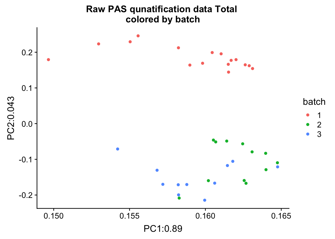

Nuclear

Run PCA on the Nuclear coverage

pca_nuc_peak=prcomp(nuclear_Cov, center=T,scale=T)
summary(pca_nuc_peak)

Importance of components:
                          PC1     PC2     PC3     PC4     PC5     PC6
Standard deviation     5.3861 1.87775 1.62240 0.99268 0.92998 0.63513
Proportion of Variance 0.7438 0.09041 0.06749 0.02527 0.02218 0.01034
Cumulative Proportion  0.7438 0.83425 0.90174 0.92701 0.94919 0.95953
                           PC7    PC8    PC9    PC10    PC11    PC12
Standard deviation     0.53149 0.4674 0.4095 0.36160 0.32862 0.28960
Proportion of Variance 0.00724 0.0056 0.0043 0.00335 0.00277 0.00215
Cumulative Proportion  0.96677 0.9724 0.9767 0.98003 0.98280 0.98495
                          PC13    PC14   PC15    PC16    PC17    PC18
Standard deviation     0.26862 0.25414 0.2333 0.22825 0.20329 0.19277
Proportion of Variance 0.00185 0.00166 0.0014 0.00134 0.00106 0.00095
Cumulative Proportion  0.98680 0.98845 0.9899 0.99118 0.99224 0.99320
                          PC19    PC20    PC21    PC22    PC23    PC24
Standard deviation     0.18620 0.17247 0.16092 0.14244 0.13630 0.12741
Proportion of Variance 0.00089 0.00076 0.00066 0.00052 0.00048 0.00042
Cumulative Proportion  0.99409 0.99485 0.99551 0.99603 0.99651 0.99693
                          PC25    PC26    PC27    PC28    PC29    PC30
Standard deviation     0.12025 0.11377 0.11306 0.10563 0.10228 0.09219
Proportion of Variance 0.00037 0.00033 0.00033 0.00029 0.00027 0.00022
Cumulative Proportion  0.99730 0.99763 0.99796 0.99824 0.99851 0.99873
                          PC31    PC32    PC33    PC34    PC35    PC36
Standard deviation     0.08916 0.08768 0.08144 0.07916 0.07412 0.07253
Proportion of Variance 0.00020 0.00020 0.00017 0.00016 0.00014 0.00013
Cumulative Proportion  0.99893 0.99913 0.99930 0.99946 0.99960 0.99974
                          PC37    PC38    PC39
Standard deviation     0.06394 0.05721 0.05416
Proportion of Variance 0.00010 0.00008 0.00008
Cumulative Proportion  0.99984 0.99992 1.00000

pca_nuc_df=as.data.frame(pca_nuc_peak$rotation) %>% rownames_to_column(var="lib") %>% mutate(line=substr(lib,2,6))
pca_nuc_df$line=as.integer(pca_nuc_df$line)

I want to color these by library size.

map_stat_nuclear=map_stats %>% filter(fraction=="nuclear")
map_stat_nuclear$batch=as.factor(map_stat_nuclear$batch)

Join the relevant stats with the pca dataframe.

pca_nuc_df=pca_nuc_df %>% full_join(map_stat_nuclear, by="line")

Plot this PCA:

ggplot(pca_nuc_df, aes(x=PC1, y=PC2, col=batch )) + geom_point() + labs(x="PC1: 0.74", y="PC2: 0.09", title="Raw PAS qunatification data nuclear \n colored by batch ")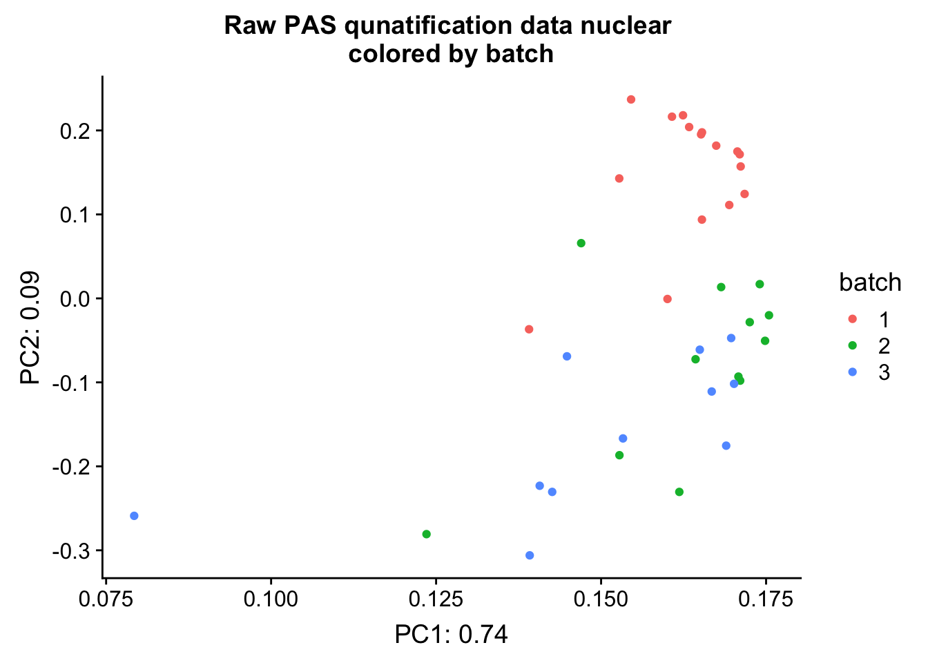

This shows that PC 2 is highly corrleated with batch,

ggplot(pca_nuc_df, aes(x=PC1, y=PC2, col=comb_mapped )) + geom_point() + labs(x="PC1: 0.74", y="PC2: 0.09", title="Raw PAS qunatification data nuclear \n colored by Mapped Read count")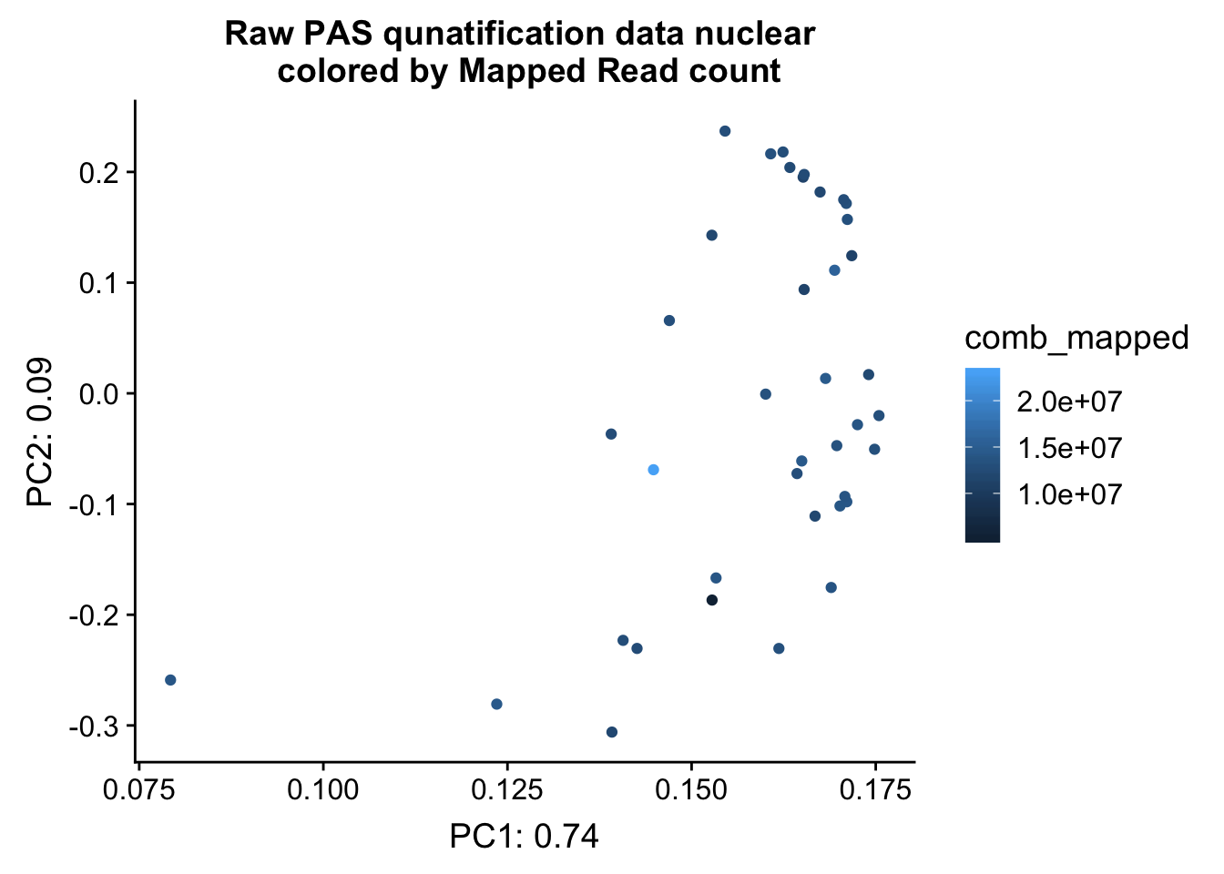

Session information

sessionInfo()

R version 3.5.1 (2018-07-02)
Platform: x86_64-apple-darwin15.6.0 (64-bit)
Running under: macOS  10.14.1

Matrix products: default
BLAS: /Library/Frameworks/R.framework/Versions/3.5/Resources/lib/libRblas.0.dylib
LAPACK: /Library/Frameworks/R.framework/Versions/3.5/Resources/lib/libRlapack.dylib

locale:
[1] en_US.UTF-8/en_US.UTF-8/en_US.UTF-8/C/en_US.UTF-8/en_US.UTF-8

attached base packages:
[1] stats     graphics  grDevices utils     datasets  methods   base     

other attached packages:
 [1] bindrcpp_0.2.2  devtools_1.13.6 reshape2_1.4.3  cowplot_0.9.3  
 [5] workflowr_1.1.1 forcats_0.3.0   stringr_1.3.1   dplyr_0.7.6    
 [9] purrr_0.2.5     readr_1.1.1     tidyr_0.8.1     tibble_1.4.2   
[13] ggplot2_3.0.0   tidyverse_1.2.1

loaded via a namespace (and not attached):
 [1] tidyselect_0.2.4  haven_1.1.2       lattice_0.20-35  
 [4] colorspace_1.3-2  htmltools_0.3.6   yaml_2.2.0       
 [7] rlang_0.2.2       R.oo_1.22.0       pillar_1.3.0     
[10] glue_1.3.0        withr_2.1.2       R.utils_2.7.0    
[13] modelr_0.1.2      readxl_1.1.0      bindr_0.1.1      
[16] plyr_1.8.4        munsell_0.5.0     gtable_0.2.0     
[19] cellranger_1.1.0  rvest_0.3.2       R.methodsS3_1.7.1
[22] memoise_1.1.0     evaluate_0.11     labeling_0.3     
[25] knitr_1.20        broom_0.5.0       Rcpp_0.12.19     
[28] scales_1.0.0      backports_1.1.2   jsonlite_1.5     
[31] hms_0.4.2         digest_0.6.17     stringi_1.2.4    
[34] grid_3.5.1        rprojroot_1.3-2   cli_1.0.1        
[37] tools_3.5.1       magrittr_1.5      lazyeval_0.2.1   
[40] crayon_1.3.4      whisker_0.3-2     pkgconfig_2.0.2  
[43] xml2_1.2.0        lubridate_1.7.4   assertthat_0.2.0 
[46] rmarkdown_1.10    httr_1.3.1        rstudioapi_0.8   
[49] R6_2.3.0          nlme_3.1-137      git2r_0.23.0     
[52] compiler_3.5.1

This reproducible R Markdown analysis was created with workflowr 1.1.1

Understand Peaks

Briana Mittleman

12/5/2018

Variation in peaks

Total:

Nuclear

Session information