QC on apaQTLs
Briana Mittleman
2/6/2019
Last updated: 2019-02-14
workflowr checks: (Click a bullet for more information)-
✔ R Markdown file: up-to-date
Great! Since the R Markdown file has been committed to the Git repository, you know the exact version of the code that produced these results.
-
✔ Environment: empty
Great job! The global environment was empty. Objects defined in the global environment can affect the analysis in your R Markdown file in unknown ways. For reproduciblity it’s best to always run the code in an empty environment.
-
✔ Seed:
set.seed(12345)The command
set.seed(12345)was run prior to running the code in the R Markdown file. Setting a seed ensures that any results that rely on randomness, e.g. subsampling or permutations, are reproducible. -
✔ Session information: recorded
Great job! Recording the operating system, R version, and package versions is critical for reproducibility.
-
Great! You are using Git for version control. Tracking code development and connecting the code version to the results is critical for reproducibility. The version displayed above was the version of the Git repository at the time these results were generated.✔ Repository version: d09198c
Note that you need to be careful to ensure that all relevant files for the analysis have been committed to Git prior to generating the results (you can usewflow_publishorwflow_git_commit). workflowr only checks the R Markdown file, but you know if there are other scripts or data files that it depends on. Below is the status of the Git repository when the results were generated:
Note that any generated files, e.g. HTML, png, CSS, etc., are not included in this status report because it is ok for generated content to have uncommitted changes.Ignored files: Ignored: .DS_Store Ignored: .Rhistory Ignored: .Rproj.user/ Ignored: data/.DS_Store Ignored: data/perm_QTL_trans_noMP_5percov/ Ignored: output/.DS_Store Untracked files: Untracked: KalistoAbundance18486.txt Untracked: analysis/4suDataIGV.Rmd Untracked: analysis/DirectionapaQTL.Rmd Untracked: analysis/EvaleQTLs.Rmd Untracked: analysis/YL_QTL_test.Rmd Untracked: analysis/ncbiRefSeq_sm.sort.mRNA.bed Untracked: analysis/snake.config.notes.Rmd Untracked: analysis/verifyBAM.Rmd Untracked: analysis/verifybam_dubs.Rmd Untracked: code/PeaksToCoverPerReads.py Untracked: code/strober_pc_pve_heatmap_func.R Untracked: data/18486.genecov.txt Untracked: data/APApeaksYL.total.inbrain.bed Untracked: data/ApaQTLs/ Untracked: data/ChromHmmOverlap/ Untracked: data/DistTXN2Peak_genelocAnno/ Untracked: data/GM12878.chromHMM.bed Untracked: data/GM12878.chromHMM.txt Untracked: data/LianoglouLCL/ Untracked: data/LocusZoom/ Untracked: data/NuclearApaQTLs.txt Untracked: data/PeakCounts/ Untracked: data/PeakCounts_noMP_5perc/ Untracked: data/PeakCounts_noMP_genelocanno/ Untracked: data/PeakUsage/ Untracked: data/PeakUsage_noMP/ Untracked: data/PeakUsage_noMP_GeneLocAnno/ Untracked: data/PeaksUsed/ Untracked: data/PeaksUsed_noMP_5percCov/ Untracked: data/RNAkalisto/ Untracked: data/RefSeq_annotations/ Untracked: data/TotalApaQTLs.txt Untracked: data/Totalpeaks_filtered_clean.bed Untracked: data/UnderstandPeaksQC/ Untracked: data/WASP_STAT/ Untracked: data/YL-SP-18486-T-combined-genecov.txt Untracked: data/YL-SP-18486-T_S9_R1_001-genecov.txt Untracked: data/YL_QTL_test/ Untracked: data/apaExamp/ Untracked: data/apaQTL_examp_noMP/ Untracked: data/bedgraph_peaks/ Untracked: data/bin200.5.T.nuccov.bed Untracked: data/bin200.Anuccov.bed Untracked: data/bin200.nuccov.bed Untracked: data/clean_peaks/ Untracked: data/comb_map_stats.csv Untracked: data/comb_map_stats.xlsx Untracked: data/comb_map_stats_39ind.csv Untracked: data/combined_reads_mapped_three_prime_seq.csv Untracked: data/diff_iso_GeneLocAnno/ Untracked: data/diff_iso_proc/ Untracked: data/diff_iso_trans/ Untracked: data/ensemble_to_genename.txt Untracked: data/example_gene_peakQuant/ Untracked: data/explainProtVar/ Untracked: data/filtPeakOppstrand_cov_noMP_GeneLocAnno_5perc/ Untracked: data/filtered_APApeaks_merged_allchrom_refseqTrans.closest2End.bed Untracked: data/filtered_APApeaks_merged_allchrom_refseqTrans.closest2End.noties.bed Untracked: data/first50lines_closest.txt Untracked: data/gencov.test.csv Untracked: data/gencov.test.txt Untracked: data/gencov_zero.test.csv Untracked: data/gencov_zero.test.txt Untracked: data/gene_cov/ Untracked: data/joined Untracked: data/leafcutter/ Untracked: data/merged_combined_YL-SP-threeprimeseq.bg Untracked: data/molPheno_noMP/ Untracked: data/mol_overlap/ Untracked: data/mol_pheno/ Untracked: data/nom_QTL/ Untracked: data/nom_QTL_opp/ Untracked: data/nom_QTL_trans/ Untracked: data/nuc6up/ Untracked: data/nuc_10up/ Untracked: data/other_qtls/ Untracked: data/pQTL_otherphen/ Untracked: data/peakPerRefSeqGene/ Untracked: data/perm_QTL/ Untracked: data/perm_QTL_GeneLocAnno_noMP_5percov/ Untracked: data/perm_QTL_GeneLocAnno_noMP_5percov_3UTR/ Untracked: data/perm_QTL_opp/ Untracked: data/perm_QTL_trans/ Untracked: data/perm_QTL_trans_filt/ Untracked: data/protAndAPAAndExplmRes.Rda Untracked: data/protAndAPAlmRes.Rda Untracked: data/protAndExpressionlmRes.Rda Untracked: data/reads_mapped_three_prime_seq.csv Untracked: data/smash.cov.results.bed Untracked: data/smash.cov.results.csv Untracked: data/smash.cov.results.txt Untracked: data/smash_testregion/ Untracked: data/ssFC200.cov.bed Untracked: data/temp.file1 Untracked: data/temp.file2 Untracked: data/temp.gencov.test.txt Untracked: data/temp.gencov_zero.test.txt Untracked: data/threePrimeSeqMetaData.csv Untracked: data/threePrimeSeqMetaData55Ind.txt Untracked: data/threePrimeSeqMetaData55Ind.xlsx Untracked: data/threePrimeSeqMetaData55Ind_noDup.txt Untracked: data/threePrimeSeqMetaData55Ind_noDup.xlsx Untracked: data/threePrimeSeqMetaData55Ind_noDup_WASPMAP.txt Untracked: data/threePrimeSeqMetaData55Ind_noDup_WASPMAP.xlsx Untracked: output/picard/ Untracked: output/plots/ Untracked: output/qual.fig2.pdf Unstaged changes: Modified: analysis/28ind.peak.explore.Rmd Modified: analysis/ApproachForGeneAssignment.Rmd Modified: analysis/CompareLianoglouData.Rmd Modified: analysis/apaQTLoverlapGWAS.Rmd Modified: analysis/cleanupdtseq.internalpriming.Rmd Modified: analysis/coloc_apaQTLs_protQTLs.Rmd Modified: analysis/dif.iso.usage.leafcutter.Rmd Modified: analysis/diff_iso_pipeline.Rmd Modified: analysis/explainpQTLs.Rmd Modified: analysis/explore.filters.Rmd Modified: analysis/flash2mash.Rmd Modified: analysis/mispriming_approach.Rmd Modified: analysis/overlapMolQTL.Rmd Modified: analysis/overlapMolQTL.opposite.Rmd Modified: analysis/overlap_qtls.Rmd Modified: analysis/peakOverlap_oppstrand.Rmd Modified: analysis/peakQCPPlots.Rmd Modified: analysis/pheno.leaf.comb.Rmd Modified: analysis/pipeline_55Ind.Rmd Modified: analysis/swarmPlots_QTLs.Rmd Modified: analysis/test.max2.Rmd Modified: analysis/understandPeaks.Rmd Modified: code/Snakefile
Expand here to see past versions:
I will use this to look at some metrics around the the QTLs from the pipeline for all 55 individuals. In this analysis I found 363 qtls in the total fraction and 623 in the nuclear.
library(workflowr)This is workflowr version 1.1.1
Run ?workflowr for help getting startedlibrary(tidyverse)── Attaching packages ───────────────────────────────────────────────────────────── tidyverse 1.2.1 ──✔ ggplot2 3.0.0 ✔ purrr 0.2.5
✔ tibble 1.4.2 ✔ dplyr 0.7.6
✔ tidyr 0.8.1 ✔ stringr 1.3.1
✔ readr 1.1.1 ✔ forcats 0.3.0── Conflicts ──────────────────────────────────────────────────────────────── tidyverse_conflicts() ──
✖ dplyr::filter() masks stats::filter()
✖ dplyr::lag() masks stats::lag()totQTLs=read.table("../data/perm_QTL_GeneLocAnno_noMP_5percov/filtered_APApeaks_merged_allchrom_refseqGenes.GeneLocAnno.NoMP_sm_quant.Total.fixed.pheno_5perc_permResBH.txt", stringsAsFactors = F, header=T)%>% filter(-log10(bh)>=1)
write.table(totQTLs,"../data/ApaQTLs/TotalapaQTLs.GeneLocAnno.noMP.5perc.10FDR.txt", row.names = F, col.names = F, quote = F)
nucQTLs=read.table("../data/perm_QTL_GeneLocAnno_noMP_5percov/filtered_APApeaks_merged_allchrom_refseqGenes.GeneLocAnno.NoMP_sm_quant.Nuclear.fixed.pheno_5perc_permResBH.txt", stringsAsFactors = F, header=T)%>% filter(-log10(bh)>=1)
write.table(nucQTLs,"../data/ApaQTLs/NuclearapaQTLs.GeneLocAnno.noMP.5perc.10FDR.txt", row.names = F, col.names = F, quote = F)Distance to end of PAS
I want to look at the distance between the QTL snp and the end of a peak. For a positive strand gene this is the end of the peak, for a - strand gene this is the start position of the peak. The peak strand here is opposite of the strand the gene is on.
I will make a python script that will take make the distance file for both the total and nucelar.
I copied these files to /project2/gilad/briana/threeprimeseq/data/ApaQTLs. I will put the QC files here as well.
getDistPeakEnd2QTL.py
#usage getDistPeakEnd2QTL.py "Total" or getDistPeakEnd2QTL.py "Nuclear"


def main(inFile, outFile):
   iFile=open(inFile, "r")
   oFile=open(outFile, "w")
   oFile.write("PeakID\tPeakEnd\tGene\tGeneStrand\tSNP_chr\tSNP_loc\tEffectSize\tBH\tDistance\n")
   for ln in iFile:
      pid= ln.split()[0]
      peakStrand=pid.split(":")[3].split("_")[1]
      if peakStrand=="+":
          strand = "-"
          end = int(pid.split(":")[1])
      else:
          strand = "+"
          end = int(pid.split(":")[2])
      gene=pid.split(":")[3].split("_")[0]
      peak=pid.split(":")[3].split("_")[2]
      SNP_Chr=ln.split()[5].split(":")[0]
      SNP_loc=int(ln.split()[5].split(":")[1])
      effectSize=ln.split()[8]
      BH=ln.split()[11]
      Dist= end - SNP_loc
      oFile.write("%s\t%d\t%s\t%s\t%s\t%d\t%s\t%s\t%d\n"%(peak, end, gene, strand, SNP_Chr, SNP_loc, effectSize, BH, Dist))
   oFile.close()


if __name__ == "__main__":
    import sys
    fraction = sys.argv[1]
    inFile = "/project2/gilad/briana/threeprimeseq/data/ApaQTLs/%sapaQTLs.GeneLocAnno.noMP.5perc.10FDR.txt"%(fraction)
    outFile = "/project2/gilad/briana/threeprimeseq/data/ApaQTLs/Distance2EndPeak.%s.apaQTLs.txt"%(fraction)
    main(inFile, outFile)
Plot for total:
TotDist=read.table("../data/ApaQTLs/Distance2EndPeak.Total.apaQTLs.txt", header=T) %>% mutate(Fraction="Total") %>% select(Fraction, Distance)
NucDist=read.table("../data/ApaQTLs/Distance2EndPeak.Nuclear.apaQTLs.txt", header=T)%>% mutate(Fraction="Nuclear") %>% select(Fraction, Distance)

BothDist=data.frame(rbind(TotDist, NucDist))
ggplot(BothDist, aes(x=Distance, by=Fraction, fill=Fraction))+geom_histogram(bins=70, alpha=.5) + scale_fill_manual(values=c("deepskyblue3","darkviolet")) + labs(title="Distance From apaQTL to End of Peak" )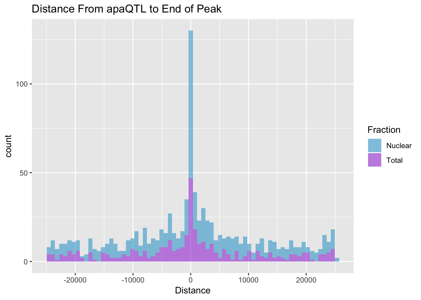
Expand here to see past versions of unnamed-chunk-5-1.png:
| Version | Author | Date |
|---|---|---|
| 450b389 | Briana Mittleman | 2019-02-06 |
Where are the SNP
I want to take all of the SNP locations see what region of the genome they are in. I can use the annotation in /project2/gilad/briana/genome_anotation_data/RefSeq_annotations/ncbiRefSeq_FormatedallAnnotation.sort.bed. I can do this with bedtools intersect if I make a bedfile for the QTLs.
Goal file: chr, loc -1, loc, peak:QTLgene, BH, geneStrand
I can get all of this information most easily from the distance file I made.
QTLfile2Bed.py
#usage QTLfile2Bed.py "Total" or QTLfile2Bed.py "Nuclear"


def main(inFile, outFile):
   iFile=open(inFile, "r")
   oFile=open(outFile, "w")
   for num, ln in enumerate(iFile):
       if num > 0:
           peakID, peakend, gene, strand, chr, loc, effect, bh, dist = ln.split()
           start=int(loc) -1
           end= int(loc)
           name= peakID + ":" + gene
           oFile.write("%s\t%d\t%d\t%s\t%s\t%s\n"%(chr, start, end, name, bh, strand))
   oFile.close()


if __name__ == "__main__":
    import sys
    fraction = sys.argv[1]
    inFile = "/project2/gilad/briana/threeprimeseq/data/ApaQTLs/Distance2EndPeak.%s.apaQTLs.txt"%(fraction)
    outFile = "/project2/gilad/briana/threeprimeseq/data/ApaQTLs/%s.apaQTLs.bed"%(fraction)
    main(inFile, outFile)
I will need to sort the output
sort -k1,1 -k2,2n /project2/gilad/briana/threeprimeseq/data/ApaQTLs/Total.apaQTLs.bed > /project2/gilad/briana/threeprimeseq/data/ApaQTLs/Total.apaQTLs.sort.bed

sort -k1,1 -k2,2n /project2/gilad/briana/threeprimeseq/data/ApaQTLs/Nuclear.apaQTLs.bed > /project2/gilad/briana/threeprimeseq/data/ApaQTLs/Nuclear.apaQTLs.sort.bed
Look at which regions these map to.
mapQTLs2GenomeLoc.sh
#!/bin/bash

#SBATCH --job-name=mapQTLs2GenomeLoc
#SBATCH --account=pi-yangili1
#SBATCH --time=24:00:00
#SBATCH --output=mapQTLs2GenomeLoc.out
#SBATCH --error=mapQTLs2GenomeLoc.err
#SBATCH --partition=broadwl
#SBATCH --mem=12G
#SBATCH --mail-type=END

module load Anaconda3
source activate three-prime-env

#annotation: /project2/gilad/briana/genome_anotation_data/RefSeq_annotations/ncbiRefSeq_FormatedallAnnotation.sort.bed

#QTL nucelar: /project2/gilad/briana/threeprimeseq/data/ApaQTLs/Nuclear.apaQTLs.sort.bed

#QTL total: /project2/gilad/briana/threeprimeseq/data/ApaQTLs/Total.apaQTLs.sort.bed


bedtools map -a /project2/gilad/briana/threeprimeseq/data/ApaQTLs/Nuclear.apaQTLs.sort.bed -b /project2/gilad/briana/genome_anotation_data/RefSeq_annotations/ncbiRefSeq_FormatedallAnnotation.sort.bed -c 4 -S -o distinct > /project2/gilad/briana/threeprimeseq/data/ApaQTLs/Nuclear.apaQTLs.sort_GeneAnno.bed


bedtools map -a /project2/gilad/briana/threeprimeseq/data/ApaQTLs/Total.apaQTLs.sort.bed -b /project2/gilad/briana/genome_anotation_data/RefSeq_annotations/ncbiRefSeq_FormatedallAnnotation.sort.bed -c 4 -S -o distinct > /project2/gilad/briana/threeprimeseq/data/ApaQTLs/Total.apaQTLs.sort_GeneAnno.bed
Most of the QTLs are not in any region.
QTLs by coverage
TotalCounts_AllInd=read.table("../data/filtPeakOppstrand_cov_noMP_GeneLocAnno_5perc/filtered_APApeaks_merged_allchrom_refseqGenes.GeneLocAnno_NoMP_sm_quant.Total.fixed.5perc.fc", header=T, stringsAsFactors = F) %>% separate(Geneid, into =c('peak', 'chr', 'start', 'end', 'strand', 'gene'), sep = ":") %>% select(-peak, -chr, -start, -end, -strand, -Chr, -Start, -End, -Strand, -Length, -gene) %>% rowMeans()

TotalCounts_AllInd_genes=read.table("../data/filtPeakOppstrand_cov_noMP_GeneLocAnno_5perc/filtered_APApeaks_merged_allchrom_refseqGenes.GeneLocAnno_NoMP_sm_quant.Total.fixed.5perc.fc", header=T, stringsAsFactors = F) %>% separate(Geneid, into =c('peak', 'chr', 'start', 'end', 'strand', 'gene'), sep = ":") %>% select(gene)


TotalCounts_AllInd_mean=data.frame(cbind(Gene=TotalCounts_AllInd_genes,Exp=TotalCounts_AllInd)) %>% filter(Exp>0)
#remove 0


TotalCounts_no0_perc= TotalCounts_AllInd_mean %>% mutate(Percentile = percent_rank(Exp))

#Seperate by percentile
TotalCounts_no0_perc10= TotalCounts_no0_perc %>% filter(Percentile<.1)

TotalCounts_no0_perc20= TotalCounts_no0_perc %>% filter(Percentile<.2& Percentile>.1)

TotalCounts_no0_perc30= TotalCounts_no0_perc %>% filter(Percentile<.3& Percentile>.2)

TotalCounts_no0_perc40= TotalCounts_no0_perc %>% filter(Percentile<.4& Percentile>.3)

TotalCounts_no0_perc50= TotalCounts_no0_perc %>% filter(Percentile<.5& Percentile>.4)
TotalCounts_no0_perc60= TotalCounts_no0_perc %>% filter(Percentile<.6& Percentile>.5)

TotalCounts_no0_perc70= TotalCounts_no0_perc %>% filter(Percentile<.7& Percentile>.6)

TotalCounts_no0_perc80= TotalCounts_no0_perc %>% filter(Percentile <.8 & Percentile>.7)
TotalCounts_no0_perc90= TotalCounts_no0_perc %>% filter(Percentile<.9 & Percentile>.8)

TotalCounts_no0_perc100= TotalCounts_no0_perc %>% filter( Percentile>.9)
Now I need to figure out the number of QTL gene in each percentile.
nucQTLGenes=nucQTLs %>% separate(pid, into=c('chr', 'start', 'end', 'id'), sep=":") %>% separate(id, sep="_", into=c("gene", 'strand', 'peak')) %>% select(gene) %>% unique()

totQTLGenes=totQTLs %>% separate(pid, into=c('chr', 'start', 'end', 'id'), sep=":") %>% separate(id, sep="_", into=c("gene", 'strand', 'peak')) %>% select(gene) %>% unique()
Per percent- use
totGene10= totQTLGenes %>% semi_join(TotalCounts_no0_perc10,by="gene") %>%  nrow()
totGene20= totQTLGenes %>% semi_join(TotalCounts_no0_perc20,by="gene")%>%  nrow()
totGene30= totQTLGenes %>% semi_join(TotalCounts_no0_perc30,by="gene")%>%  nrow()
totGene40= totQTLGenes %>% semi_join(TotalCounts_no0_perc40,by="gene")%>% nrow()
totGene50= totQTLGenes %>% semi_join(TotalCounts_no0_perc50,by="gene")%>% nrow()
totGene60= totQTLGenes %>% semi_join(TotalCounts_no0_perc60,by="gene")%>% nrow()
totGene70= totQTLGenes %>% semi_join(TotalCounts_no0_perc70,by="gene")%>%  nrow()
totGene80= totQTLGenes %>% semi_join(TotalCounts_no0_perc80,by="gene")%>%  nrow()
totGene90= totQTLGenes %>% semi_join(TotalCounts_no0_perc90,by="gene")%>%  nrow()
totGene100= totQTLGenes %>% semi_join(TotalCounts_no0_perc100,by="gene")%>%  nrow()


totGene_allPerc=c(totGene10,totGene20,totGene30,totGene40,totGene50,totGene60,totGene70,totGene80, totGene90,totGene100)
plot this:
plot(totGene_allPerc)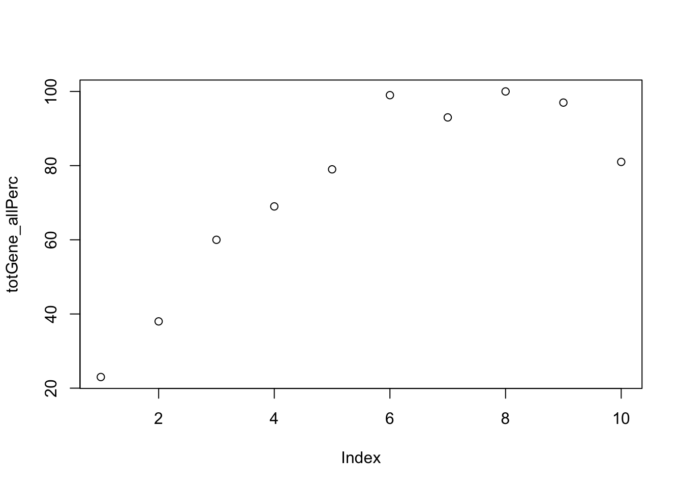 Why are more genes included
Session information
sessionInfo()R version 3.5.1 (2018-07-02)
Platform: x86_64-apple-darwin15.6.0 (64-bit)
Running under: macOS 10.14.1
Matrix products: default
BLAS: /Library/Frameworks/R.framework/Versions/3.5/Resources/lib/libRblas.0.dylib
LAPACK: /Library/Frameworks/R.framework/Versions/3.5/Resources/lib/libRlapack.dylib
locale:
[1] en_US.UTF-8/en_US.UTF-8/en_US.UTF-8/C/en_US.UTF-8/en_US.UTF-8
attached base packages:
[1] stats graphics grDevices utils datasets methods base
other attached packages:
[1] bindrcpp_0.2.2 forcats_0.3.0 stringr_1.3.1 dplyr_0.7.6
[5] purrr_0.2.5 readr_1.1.1 tidyr_0.8.1 tibble_1.4.2
[9] ggplot2_3.0.0 tidyverse_1.2.1 workflowr_1.1.1
loaded via a namespace (and not attached):
[1] tidyselect_0.2.4 haven_1.1.2 lattice_0.20-35
[4] colorspace_1.3-2 htmltools_0.3.6 yaml_2.2.0
[7] rlang_0.2.2 R.oo_1.22.0 pillar_1.3.0
[10] glue_1.3.0 withr_2.1.2 R.utils_2.7.0
[13] modelr_0.1.2 readxl_1.1.0 bindr_0.1.1
[16] plyr_1.8.4 munsell_0.5.0 gtable_0.2.0
[19] cellranger_1.1.0 rvest_0.3.2 R.methodsS3_1.7.1
[22] evaluate_0.11 labeling_0.3 knitr_1.20
[25] broom_0.5.0 Rcpp_0.12.19 scales_1.0.0
[28] backports_1.1.2 jsonlite_1.5 hms_0.4.2
[31] digest_0.6.17 stringi_1.2.4 grid_3.5.1
[34] rprojroot_1.3-2 cli_1.0.1 tools_3.5.1
[37] magrittr_1.5 lazyeval_0.2.1 crayon_1.3.4
[40] whisker_0.3-2 pkgconfig_2.0.2 xml2_1.2.0
[43] lubridate_1.7.4 assertthat_0.2.0 rmarkdown_1.10
[46] httr_1.3.1 rstudioapi_0.8 R6_2.3.0
[49] nlme_3.1-137 git2r_0.23.0 compiler_3.5.1
This reproducible R Markdown analysis was created with workflowr 1.1.1