Generate bigwig files and peak calling
2024-12-26
Last updated: 2024-12-27
Checks: 6 1
Knit directory:
reproduce_genomics_paper_figures/
This reproducible R Markdown analysis was created with workflowr (version 1.7.1). The Checks tab describes the reproducibility checks that were applied when the results were created. The Past versions tab lists the development history.
The R Markdown is untracked by Git. To know which version of the R
Markdown file created these results, you’ll want to first commit it to
the Git repo. If you’re still working on the analysis, you can ignore
this warning. When you’re finished, you can run
wflow_publish to commit the R Markdown file and build the
HTML.
Great job! The global environment was empty. Objects defined in the global environment can affect the analysis in your R Markdown file in unknown ways. For reproduciblity it’s best to always run the code in an empty environment.
The command set.seed(20241226) was run prior to running
the code in the R Markdown file. Setting a seed ensures that any results
that rely on randomness, e.g. subsampling or permutations, are
reproducible.
Great job! Recording the operating system, R version, and package versions is critical for reproducibility.
Nice! There were no cached chunks for this analysis, so you can be confident that you successfully produced the results during this run.
Great job! Using relative paths to the files within your workflowr project makes it easier to run your code on other machines.
Great! You are using Git for version control. Tracking code development and connecting the code version to the results is critical for reproducibility.
The results in this page were generated with repository version fc1e415. See the Past versions tab to see a history of the changes made to the R Markdown and HTML files.
Note that you need to be careful to ensure that all relevant files for
the analysis have been committed to Git prior to generating the results
(you can use wflow_publish or
wflow_git_commit). workflowr only checks the R Markdown
file, but you know if there are other scripts or data files that it
depends on. Below is the status of the Git repository when the results
were generated:
Ignored files:
    Ignored:    .DS_Store
    Ignored:    .Rproj.user/
    Ignored:    analysis/.DS_Store
    Ignored:    data/fastq/
    Ignored:    data/reference/

Untracked files:
    Untracked:  analysis/01_download_fastq_from_GEO.Rmd
    Untracked:  analysis/02_align_to_hg38.Rmd
    Untracked:  analysis/03_generate_bigwig.Rmd

Unstaged changes:
    Modified:   .gitignore
    Modified:   README.md
    Modified:   analysis/index.Rmd
    Modified:   reproduce_genomics_paper_figures.Rproj
Note that any generated files, e.g. HTML, png, CSS, etc., are not included in this status report because it is ok for generated content to have uncommitted changes.
There are no past versions. Publish this analysis with
wflow_publish() to start tracking its development.
generate bigwig files
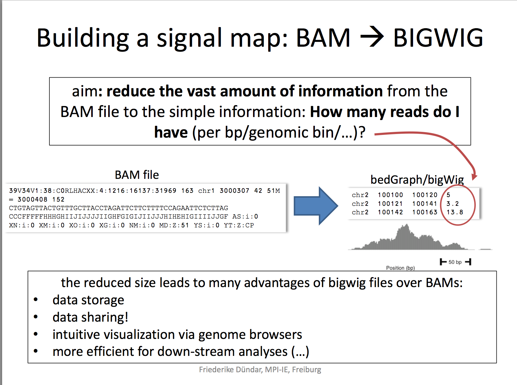
Now that we have the sorted bam file, we can generate a genome wide signal view as a bigwig file.
A BigWig file is a binary file format commonly used in bioinformatics to efficiently store and visualize continuous data over genomic coordinates, such as read coverage or signal intensity. It is derived from the Wiggle (WIG) format but optimized for faster access and reduced file size, making it suitable for large-scale genomic data.
UCSC has a detailed page explaining what is it https://genome.ucsc.edu/goldenpath/help/bigWig.html
Bonus: Bioinformatics is nortorious about different file formats. read https://genome.ucsc.edu/FAQ/FAQformat.html for various formats definitions
For this purpose, we will use deeptools https://deeptools.readthedocs.io/en/develop/content/example_usage.html
deeptools is very versatile and it has many sub-commands.
We will use bamCoverage to generate bigwig files.
# install it via conda if you do not have it yet
conda install -c conda-forge -c bioconda deeptools
# or
pip install deeptools
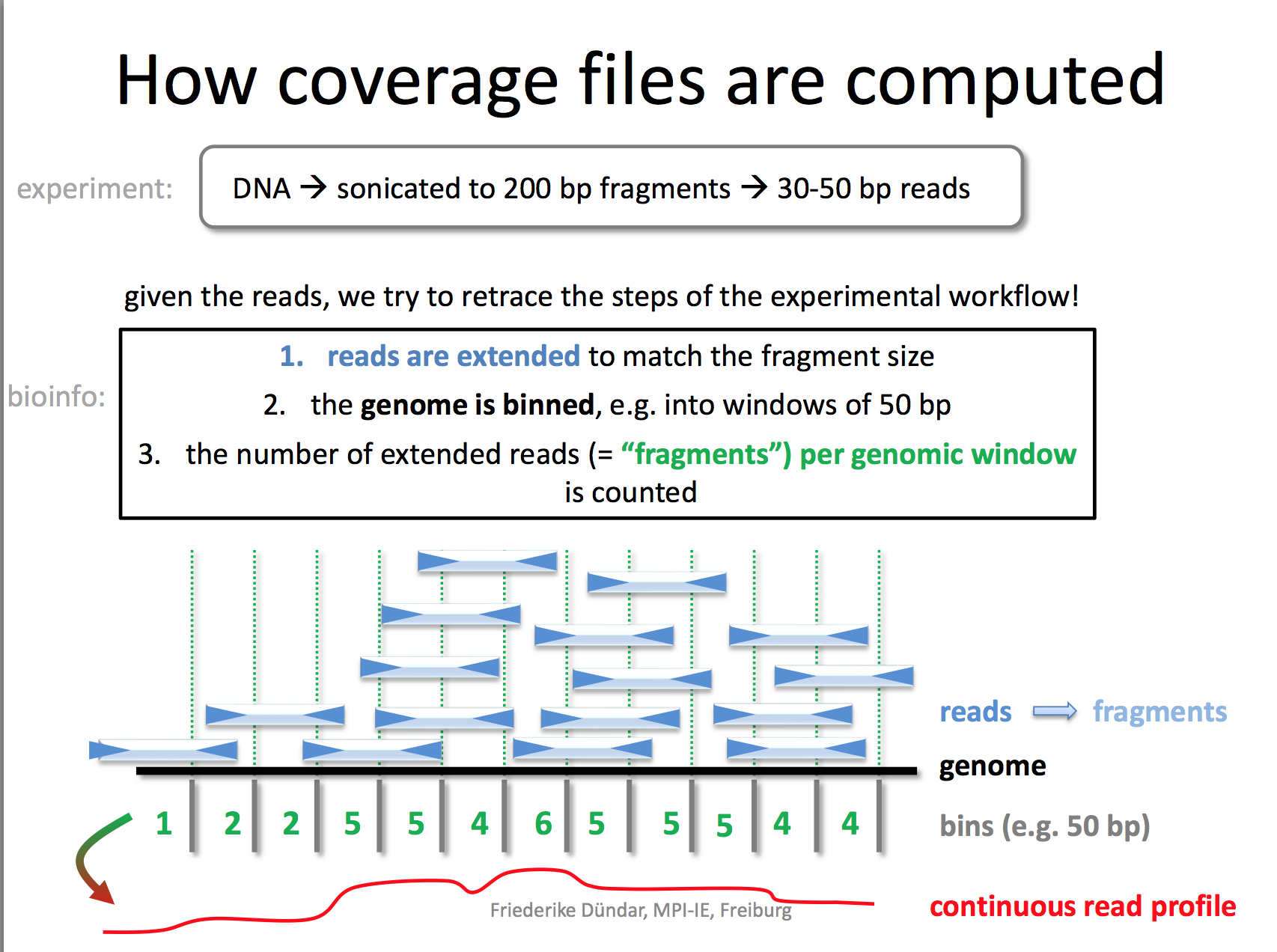
I really like the demonstration of how coverage files are computed by the deeptools authors.
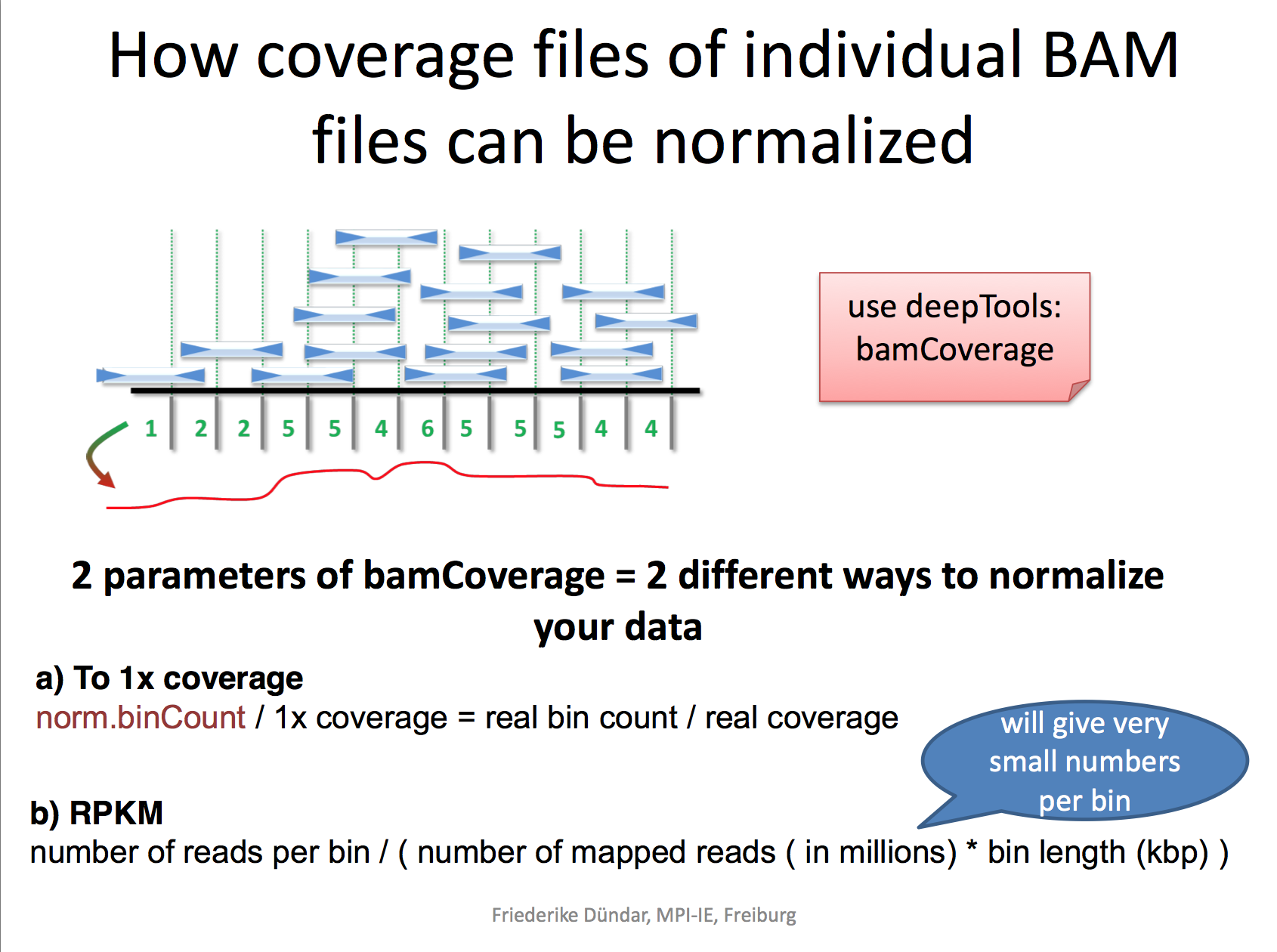
RPKM: reads per kilobase per million reads The formula is: RPKM (per bin) = number of reads per bin /(number of mapped reads (in millions) * bin length (kp))
RPGC: reads per genomic content used to normalize reads to 1x depth of coverage sequencing depth is defined as: (total number of mapped reads * fragment length) / effective genome size
cd data/fastq
bamCoverage --bam YAP.sorted.bam --normalizeUsing RPKM --extendReads 200 -o YAP1.bw
Read here to understand why you need to extend the reads to 200 bp. We only sequenced 50bp of the DNA after antibody pull-down, but the real DNA is about 200 bp (the size of the DNA after sonication/fragmentation)
We used default bin size 50 bp.
Generate bigwig files for all samples
for bam in *sorted.bam
do
  bamCoverage --bam $bam --normalizeUsing RPKM --extendReads 200 -o ${bam/sorted.bam/bw}
done
peak calling
MACS
is the most popular peak caller for ChIPseq. It is maintained by Tao
Liu. I had the pleasure working with him on some single-cell ATACseq
stuff when I was in Shirley Liu’s lab.
MACS is now MACS3! https://macs3-project.github.io/MACS/docs/INSTALL.html
pip install --upgrade macs3The MACS3 callpeak subcommands have many paramters and you want to read https://macs3-project.github.io/MACS/docs/callpeak.html
macs3 callpeak -t YAP.sorted.bam -c IgG.sorted.bam -f BAM -n YAP -g hs --outdir YAP_peakIt takes a couple of minutes. output:
ls YAP_peak/
YAP1_model.r          YAP1_peaks.narrowPeak YAP1_peaks.xls        YAP1_summits.bed
Do it for all samples
for bam in *sorted.bam
do
  macs3 callpeak -t $bam -c IgG.sorted.bam -f BAM -n ${bam%.sorted.bam} -g hs --outdir ${bam/.sorted.bam/_peak}
done
What is Model Building in MACS?
Model building in MACS (Model-Based Analysis of ChIP-Seq) is a step that attempts to determine the average fragment size of DNA fragments from sequencing data. It uses the shifted positions of the tags (forward and reverse reads) to estimate the peak signal. The estimated fragment size is then used to build a model of the peak shape, which is important for identifying and refining peak regions.
Model Building: Single-End vs. Paired-End
- Single-End Data:
Model building is used because the fragment size is not directly available from single-end reads. MACS shifts the reads by half the estimated fragment size to align them to the putative binding sites.
- Paired-End Data:
Model building is usually not needed because the fragment size is directly available from the paired-end read alignment. In paired-end mode, MACS calculates the actual insert size between read pairs, bypassing the need for model building.
When to Use –no-model and –extend-size
For single-end data, you might use –no-model and –extend-size in specific scenarios where you want to skip model building and manually specify the fragment size:
–no-model:
Disables the model building step. Use this option if you already know the approximate fragment size from your library preparation.
–extend-size:
Extends reads to the specified fragment size (e.g., 200 bp). This mimics the actual fragment length in the absence of paired-end information.
Best Practices for Single-End Data
- With Model Building (Default Behavior):
Let MACS build the model unless there are specific reasons to disable it.
macs2 callpeak -t treatment.bam -c control.bam -f BED -g hs -n sample –outdir results
- Without Model Building (–no-model):
Use when: You know the fragment size (e.g., from library preparation or empirical testing). The library is not suitable for accurate model building (e.g., very low read depth or noisy data). Specify –extend-size to set the fragment size.
macs2 callpeak -t treatment.bam -c control.bam -f BED -g hs -n sample --outdir results --no-model --extend-size 200
Why Use –no-model and –extend-size for Single-End?
Consistency: You can ensure the fragment size is consistently applied across all datasets. Noise Reduction: Avoid errors from noisy or low-quality data affecting model estimation. Speed: Skipping model building can make peak calling faster.
Model building is relevant for single-end data and used by default
unless –no-model is specified. For paired-end data, model building is
typically unnecessary since the fragment size is directly calculated.
Use –no-model –extend-size
Challenges
The paper uses a previous generated ChIP-seq dataset https://www.ncbi.nlm.nih.gov/geo/query/acc.cgi?acc=GSE49651 for H3K4me1, H3K4me3 and H3K27ac. The authors used H3K4me1 to define enhancers and H3K4me3 to define promoters. H3K4me1/H3K27ac to define active enhancers and H3K4me3/H3K27ac to define active promoters.
Can you process the data yourself?
sessionInfo()R version 4.4.1 (2024-06-14)
Platform: aarch64-apple-darwin20
Running under: macOS Sonoma 14.1
Matrix products: default
BLAS: /Library/Frameworks/R.framework/Versions/4.4-arm64/Resources/lib/libRblas.0.dylib
LAPACK: /Library/Frameworks/R.framework/Versions/4.4-arm64/Resources/lib/libRlapack.dylib; LAPACK version 3.12.0
locale:
[1] en_US.UTF-8/en_US.UTF-8/en_US.UTF-8/C/en_US.UTF-8/en_US.UTF-8
time zone: America/New_York
tzcode source: internal
attached base packages:
[1] stats graphics grDevices utils datasets methods base
other attached packages:
[1] workflowr_1.7.1
loaded via a namespace (and not attached):
[1] vctrs_0.6.5 httr_1.4.7 cli_3.6.3 knitr_1.48
[5] rlang_1.1.4 xfun_0.46 stringi_1.8.4 processx_3.8.4
[9] promises_1.3.0 jsonlite_1.8.8 glue_1.7.0 rprojroot_2.0.4
[13] git2r_0.35.0 htmltools_0.5.8.1 httpuv_1.6.15 ps_1.7.7
[17] sass_0.4.9 fansi_1.0.6 rmarkdown_2.27 jquerylib_0.1.4
[21] tibble_3.2.1 evaluate_0.24.0 fastmap_1.2.0 yaml_2.3.10
[25] lifecycle_1.0.4 whisker_0.4.1 stringr_1.5.1 compiler_4.4.1
[29] fs_1.6.4 pkgconfig_2.0.3 Rcpp_1.0.13 rstudioapi_0.16.0
[33] later_1.3.2 digest_0.6.36 R6_2.5.1 utf8_1.2.4
[37] pillar_1.9.0 callr_3.7.6 magrittr_2.0.3 bslib_0.8.0
[41] tools_4.4.1 cachem_1.1.0 getPass_0.2-4