scRNA-seq clusters
2026-01-19
Last updated: 2026-01-19
Checks: 7 0
Knit directory: muse/
This reproducible R Markdown analysis was created with workflowr (version 1.7.1). The Checks tab describes the reproducibility checks that were applied when the results were created. The Past versions tab lists the development history.
Great! Since the R Markdown file has been committed to the Git repository, you know the exact version of the code that produced these results.
Great job! The global environment was empty. Objects defined in the global environment can affect the analysis in your R Markdown file in unknown ways. For reproduciblity it’s best to always run the code in an empty environment.
The command set.seed(20200712) was run prior to running
the code in the R Markdown file. Setting a seed ensures that any results
that rely on randomness, e.g. subsampling or permutations, are
reproducible.
Great job! Recording the operating system, R version, and package versions is critical for reproducibility.
Nice! There were no cached chunks for this analysis, so you can be confident that you successfully produced the results during this run.
Great job! Using relative paths to the files within your workflowr project makes it easier to run your code on other machines.
Great! You are using Git for version control. Tracking code development and connecting the code version to the results is critical for reproducibility.
The results in this page were generated with repository version 904fc56. See the Past versions tab to see a history of the changes made to the R Markdown and HTML files.
Note that you need to be careful to ensure that all relevant files for
the analysis have been committed to Git prior to generating the results
(you can use wflow_publish or
wflow_git_commit). workflowr only checks the R Markdown
file, but you know if there are other scripts or data files that it
depends on. Below is the status of the Git repository when the results
were generated:
Ignored files:
    Ignored:    .Rproj.user/
    Ignored:    data/1M_neurons_filtered_gene_bc_matrices_h5.h5
    Ignored:    data/293t/
    Ignored:    data/293t_3t3_filtered_gene_bc_matrices.tar.gz
    Ignored:    data/293t_filtered_gene_bc_matrices.tar.gz
    Ignored:    data/5k_Human_Donor1_PBMC_3p_gem-x_5k_Human_Donor1_PBMC_3p_gem-x_count_sample_filtered_feature_bc_matrix.h5
    Ignored:    data/5k_Human_Donor2_PBMC_3p_gem-x_5k_Human_Donor2_PBMC_3p_gem-x_count_sample_filtered_feature_bc_matrix.h5
    Ignored:    data/5k_Human_Donor3_PBMC_3p_gem-x_5k_Human_Donor3_PBMC_3p_gem-x_count_sample_filtered_feature_bc_matrix.h5
    Ignored:    data/5k_Human_Donor4_PBMC_3p_gem-x_5k_Human_Donor4_PBMC_3p_gem-x_count_sample_filtered_feature_bc_matrix.h5
    Ignored:    data/97516b79-8d08-46a6-b329-5d0a25b0be98.h5ad
    Ignored:    data/Parent_SC3v3_Human_Glioblastoma_filtered_feature_bc_matrix.tar.gz
    Ignored:    data/brain_counts/
    Ignored:    data/cl.obo
    Ignored:    data/cl.owl
    Ignored:    data/jurkat/
    Ignored:    data/jurkat:293t_50:50_filtered_gene_bc_matrices.tar.gz
    Ignored:    data/jurkat_293t/
    Ignored:    data/jurkat_filtered_gene_bc_matrices.tar.gz
    Ignored:    data/pbmc20k/
    Ignored:    data/pbmc20k_seurat/
    Ignored:    data/pbmc3k.csv
    Ignored:    data/pbmc3k.csv.gz
    Ignored:    data/pbmc3k.h5ad
    Ignored:    data/pbmc3k/
    Ignored:    data/pbmc3k_bpcells_mat/
    Ignored:    data/pbmc3k_export.mtx
    Ignored:    data/pbmc3k_matrix.mtx
    Ignored:    data/pbmc3k_seurat.rds
    Ignored:    data/pbmc4k_filtered_gene_bc_matrices.tar.gz
    Ignored:    data/pbmc_1k_v3_filtered_feature_bc_matrix.h5
    Ignored:    data/pbmc_1k_v3_raw_feature_bc_matrix.h5
    Ignored:    data/refdata-gex-GRCh38-2020-A.tar.gz
    Ignored:    data/seurat_1m_neuron.rds
    Ignored:    data/t_3k_filtered_gene_bc_matrices.tar.gz
    Ignored:    r_packages_4.4.1/
    Ignored:    r_packages_4.5.0/

Untracked files:
    Untracked:  analysis/bioc.Rmd
    Untracked:  analysis/bioc_scrnaseq.Rmd
    Untracked:  analysis/likelihood.Rmd
    Untracked:  bpcells_matrix/
    Untracked:  data/Caenorhabditis_elegans.WBcel235.113.gtf.gz
    Untracked:  data/GCF_043380555.1-RS_2024_12_gene_ontology.gaf.gz
    Untracked:  data/arab.rds
    Untracked:  data/astronomicalunit.csv
    Untracked:  data/femaleMiceWeights.csv
    Untracked:  data/lung_bcell.rds
    Untracked:  m3/
    Untracked:  women.json

Unstaged changes:
    Modified:   analysis/icc.Rmd
    Modified:   analysis/isoform_switch_analyzer.Rmd
Note that any generated files, e.g. HTML, png, CSS, etc., are not included in this status report because it is ok for generated content to have uncommitted changes.
These are the previous versions of the repository in which changes were
made to the R Markdown (analysis/scrnaseq_clusters.Rmd) and
HTML (docs/scrnaseq_clusters.html) files. If you’ve
configured a remote Git repository (see ?wflow_git_remote),
click on the hyperlinks in the table below to view the files as they
were in that past version.
| File | Version | Author | Date | Message |
|---|---|---|---|---|
| Rmd | 904fc56 | Dave Tang | 2026-01-19 | Fix formatting |
| html | 29f3c2e | Dave Tang | 2026-01-19 | Build site. |
| Rmd | ca08f19 | Dave Tang | 2026-01-19 | Evaluating scRNA-seq clusters |
Introduction
Access the heterogeneity in scRNA-seq clusters where heterogeneity refers to how variable or diverse cells are within a given cluster. High heterogeneity means cells in that cluster are quite different from each other, while low heterogeneity means they’re very similar.
Dependencies
install.packages(c("Seurat", "cluster", "pheatmap"))Seurat workflow
Import raw pbmc3k dataset from my server.
seurat_obj <- readRDS(url("https://davetang.org/file/pbmc3k_seurat.rds", "rb"))
seurat_obj
An object of class Seurat
32738 features across 2700 samples within 1 assay
Active assay: RNA (32738 features, 0 variable features)
1 layer present: countsFilter.
seurat_obj <- CreateSeuratObject(
  counts = seurat_obj@assays$RNA$counts,
  min.cells = 3,
  min.features = 200,
  project = "pbmc3k"
)
seurat_obj
An object of class Seurat
13714 features across 2700 samples within 1 assay
Active assay: RNA (13714 features, 0 variable features)
1 layer present: countsProcess with the Seurat 4 workflow.
seurat_wf_v4 <- function(seurat_obj, scale_factor = 1e4, num_features = 2000, num_pcs = 30, cluster_res = 0.5, debug_flag = FALSE){

  seurat_obj <- NormalizeData(seurat_obj, normalization.method = "LogNormalize", scale.factor = scale_factor, verbose = debug_flag)
  seurat_obj <- FindVariableFeatures(seurat_obj, selection.method = 'vst', nfeatures = num_features, verbose = debug_flag)
  seurat_obj <- ScaleData(seurat_obj, verbose = debug_flag)
  seurat_obj <- RunPCA(seurat_obj, verbose = debug_flag)
  seurat_obj <- RunUMAP(seurat_obj, dims = 1:num_pcs, verbose = debug_flag)
  seurat_obj <- FindNeighbors(seurat_obj, dims = 1:num_pcs, verbose = debug_flag)
  seurat_obj <- FindClusters(seurat_obj, resolution = cluster_res, verbose = debug_flag)

  seurat_obj
}

seurat_obj <- seurat_wf_v4(seurat_obj)
Warning: The default method for RunUMAP has changed from calling Python UMAP via reticulate to the R-native UWOT using the cosine metric
To use Python UMAP via reticulate, set umap.method to 'umap-learn' and metric to 'correlation'
This message will be shown once per sessionClusters
Cluster results are in seurat_clusters.
table(seurat_obj$seurat_clusters)
   0    1    2    3    4    5    6    7
1187  491  351  301  163  161   32   14
Silhouette Scores
What it measures: How similar each cell is to cells in its own cluster compared to cells in other clusters.
Interpretation:
- Score close to 1 = cell is very similar to its cluster and different from others (good clustering, low heterogeneity)
- Score close to 0 = cell is on the border between clusters
- Score close to -1 = cell might be in the wrong cluster
Why it matters: Higher average silhouette scores for a cluster indicate it’s well-separated and homogeneous.
The function cluster::silhouette() computes silhouette
information according to a given clustering in k clusters.
silhouette(x, dist, dmatrix, …)
where x is an object of appropriate class; for the
default method an integer vector with \(k\) different integer cluster codes or a
list with such an x$clustering component.
pca_embeddings <- Seurat::Embeddings(seurat_obj, reduction = "pca")[, 1:30]
dist_matrix <- stats::dist(pca_embeddings)
clusters <- seurat_obj$seurat_clusters
cluster_numeric <- as.numeric(clusters)
sil_scores <- cluster::silhouette(cluster_numeric, dist_matrix)

head(sil_scores)
cluster neighbor sil_width
[1,] 1 4 0.15700201
[2,] 3 1 0.22826737
[3,] 1 4 0.15604285
[4,] 6 2 -0.00517726
[5,] 5 4 -0.06343489
[6,] 1 4 0.28198441Calculate average silhouette width per cluster.
sil_scores |>
  as.data.frame() |>
  dplyr::summarise(avg_silhouette = mean(sil_width), .by = 'cluster') |>
  dplyr::arrange(-avg_silhouette) |>
  dplyr::mutate(cluster = as.factor(cluster-1)) -> sil_summary

sil_summary |> dplyr::arrange(-avg_silhouette)
cluster avg_silhouette
1 7 0.39537997
2 6 0.32047942
3 0 0.23125232
4 2 0.22471219
5 5 0.22205239
6 1 0.21488745
7 3 0.05981687
8 4 0.01407852Plot silhouette scores.
ggplot(sil_summary, aes(x = reorder(cluster, avg_silhouette), y = avg_silhouette, fill = cluster)) +
  geom_bar(stat = "identity") +
  coord_flip() +
  labs(title = "Cluster Quality: Silhouette Scores",
                subtitle = "Higher scores = more distinct/homogeneous clusters",
                x = "Cluster", y = "Average Silhouette Width") +
  theme_minimal() +
  theme(legend.position = "none")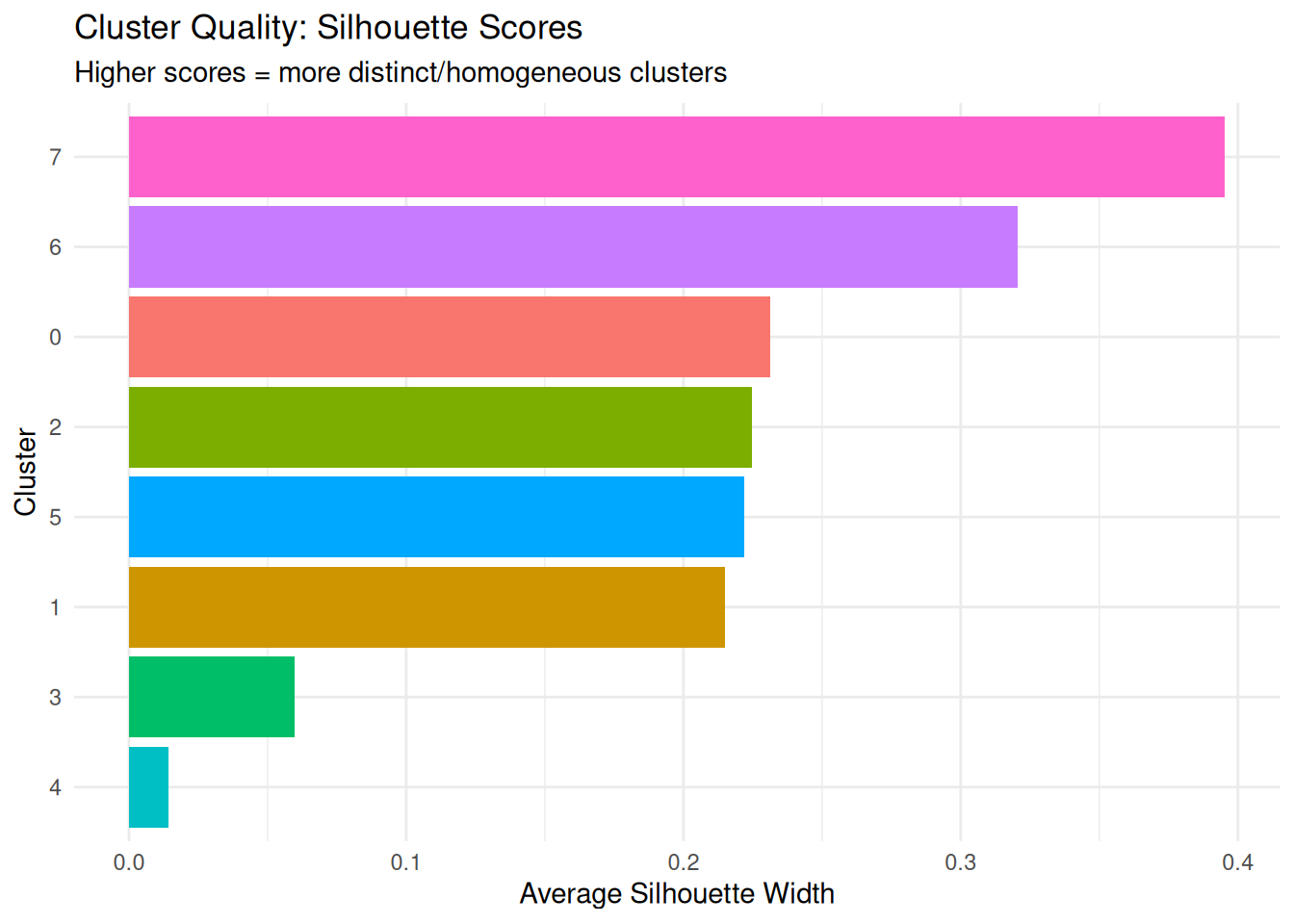
| Version | Author | Date |
|---|---|---|
| 29f3c2e | Dave Tang | 2026-01-19 |
Higher scores = more distinct/homogeneous clusters means two things:
- Distinct (well-separated from other clusters): Cells in this cluster are far away from cells in other clusters.
- Homogeneous (internally similar): Cells within this cluster are close to each other.
The silhouette score combines both concepts:
- It measures how similar a cell is to its own cluster (homogeneity)
- Compared to how similar it is to the nearest neighboring cluster (distinctness/separation)
For example a high silhouette score (e.g., 0.8) means cells in cluster A are tightly packed together AND far from cluster B -> cluster A is both homogeneous internally and well-separated from others. A low silhouette score (e.g., 0.2) means cells in cluster A are either spread out OR very close to cluster B (or both) -> poor clustering quality.
It is important to note that a cluster can have a high silhouette score for two reasons:
- Low heterogeneity (cells are very similar to each other).
- Good separation from other clusters.
Within-Cluster Variance and Coefficient of Variation
What it measures: How much gene expression varies among cells within each cluster.
Interpretation:
- Variance = absolute spread of expression values
- Coefficient of Variation (CV) = variance relative to mean (more comparable across genes)
- Higher values = more heterogeneous gene expression within the cluster
Why it matters: Some cell types naturally have more variable expression (e.g., transitioning cells) while others are more stable (e.g., terminally differentiated cells).
expr_data <- Seurat::GetAssayData(seurat_obj, assay = 'RNA', layer = "data")

variable_genes <- Seurat::VariableFeatures(seurat_obj)
expr_data <- expr_data[variable_genes, ]

# Calculate variance and CV for each cluster
variance_results <- lapply(unique(clusters), function(cl) {
  # Get cells in this cluster
  cells_in_cluster <- which(clusters == cl)
  cluster_expr <- expr_data[, cells_in_cluster]

  # Calculate metrics for each gene
  gene_means <- apply(cluster_expr, 1, mean)
  gene_vars <- apply(cluster_expr, 1, var)
  gene_cv <- sqrt(gene_vars) / (gene_means + 0.01)  # Add small constant to avoid division by zero

  data.frame(
    cluster = cl,
    mean_variance = mean(gene_vars),
    mean_cv = mean(gene_cv),
    median_variance = median(gene_vars),
    median_cv = median(gene_cv)
  )
}) |> dplyr::bind_rows()

variance_results |>
  dplyr::arrange(-mean_cv)
cluster mean_variance mean_cv median_variance median_cv
1 0 0.2053429 3.894674 0.1237998 3.863553
2 2 0.2200781 3.814635 0.1297913 3.868301
3 1 0.2279141 3.690295 0.1118532 3.849844
4 3 0.2458172 3.505332 0.1429896 3.483285
5 4 0.2849902 3.124803 0.1674329 3.012039
6 5 0.2089924 2.810056 0.1237510 2.725329
7 6 0.1883484 1.908411 0.1198264 1.850823
8 7 0.2644712 1.107976 0.0000000 0.000000Plot.
ggplot(variance_results, ggplot2::aes(x = reorder(cluster, mean_cv),
                                      y = mean_cv, fill = cluster)) +
  geom_bar(stat = "identity") +
  coord_flip() +
  labs(title = "Within-Cluster Gene Expression Variability",
       subtitle = "Higher CV = more heterogeneous expression patterns",
       x = "Cluster", y = "Mean Coefficient of Variation") +
  theme_minimal() +
  theme(legend.position = "none")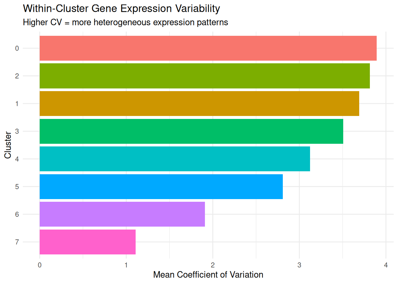
| Version | Author | Date |
|---|---|---|
| 29f3c2e | Dave Tang | 2026-01-19 |
CV (Coefficient of Variation) measures how variable gene expression is relative to the average expression level. A low CV (e.g., 0.3 or 30%): Gene expression values are tightly clustered around the mean; a high CV (e.g., 1.5 or 150%): Gene expression values are spread widely around the mean. CV is normalised by the mean, so it’s comparable across genes with different expression levels.
- High mean CV across genes: Cells in this cluster have diverse transcriptional states - they’re expressing different genes at different levels
- Low mean CV across genes: Cells in this cluster have consistent transcriptional states - they’re expressing genes at similar levels
Intra-Cluster Distances in PCA Space
What it measures: The average distance between cells within the same cluster in reduced dimension space.
Interpretation:
- Smaller distances = cells are tightly clustered together (low heterogeneity)
- Larger distances = cells are spread out (high heterogeneity)
Why it matters: This gives you a spatial sense of cluster compactness. We calculate this in both PCA (captures biological variance) and UMAP (optimized for visualization).
# Function to calculate intra-cluster distances
calc_intra_cluster_dist <- function(embeddings, labels) {
  results <- lapply(unique(labels), function(cl) {
    # Get cells in this cluster
    cells_in_cluster <- which(labels == cl)
    cluster_embeddings <- embeddings[cells_in_cluster, ]

    # Calculate all pairwise distances within cluster
    dist_within <- stats::dist(cluster_embeddings)

    data.frame(
      cluster = cl,
      n_cells = length(cells_in_cluster),
      mean_distance = mean(dist_within),
      median_distance = median(dist_within),
      sd_distance = sd(dist_within)
    )
  }) |> dplyr::bind_rows()

  return(results)
}

pca_embeddings <- Seurat::Embeddings(seurat_obj, reduction = "pca")[, 1:30]
pca_dist_summary <- calc_intra_cluster_dist(pca_embeddings, clusters)

pca_dist_summary |>
  dplyr::arrange(desc(mean_distance))
cluster n_cells mean_distance median_distance sd_distance
1 7 14 31.91325 27.64812 19.712474
2 4 163 20.08154 17.23594 10.125879
3 6 32 13.63669 13.34247 3.030101
4 3 301 13.44704 13.26069 2.547182
5 5 161 13.06556 12.72586 2.742325
6 2 351 13.05064 12.28683 4.166248
7 1 491 12.98647 12.67202 2.757599
8 0 1187 11.06922 10.73953 2.478361Plot.
ggplot(pca_dist_summary, aes(x = reorder(cluster, mean_distance),
                             y = mean_distance, fill = cluster)) +
  geom_bar(stat = "identity") +
  geom_errorbar(ggplot2::aes(ymin = mean_distance - sd_distance,
                             ymax = mean_distance + sd_distance),
                width = 0.2) +
  coord_flip() +
  labs(title = "Cluster Spread in PCA Space",
       subtitle = "Higher distance = more spread out cells = higher heterogeneity",
       x = "Cluster", y = "Mean Pairwise Distance") +
  theme_minimal() +
  theme(legend.position = "none")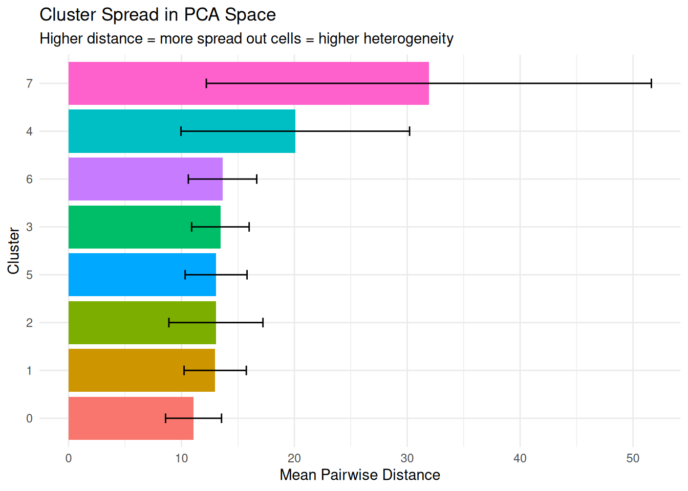
| Version | Author | Date |
|---|---|---|
| 29f3c2e | Dave Tang | 2026-01-19 |
Shannon Entropy
What it measures: The diversity of gene expression distributions within each cluster.
Interpretation:
- Higher entropy = gene expression is more evenly distributed across many values (high heterogeneity)
- Lower entropy = gene expression is concentrated around specific values (low heterogeneity)
Why it matters: Entropy captures whether cells have uniform or variable transcriptional states. It’s particularly useful for identifying transitional or stressed cell populations.
shannon_entropy <- function(x) {
  # Bin expression values into 10 bins
  breaks <- seq(min(x), max(x), length.out = 11)
  hist_data <- hist(x, breaks = breaks, plot = FALSE)

  # Calculate probability of each bin
  probs <- hist_data$counts / sum(hist_data$counts)
  probs <- probs[probs > 0]  # Remove zeros to avoid log(0)

  # Shannon entropy formula: -sum(p * log2(p))
  return(-sum(probs * log2(probs)))
}

entropy_results <- lapply(unique(clusters), function(cl) {
  # Get cells in this cluster
  cells_in_cluster <- which(clusters == cl)
  cluster_expr <- expr_data[, cells_in_cluster]

  # Calculate entropy for each gene
  gene_entropies <- apply(cluster_expr, 1, shannon_entropy)

  data.frame(
    cluster = cl,
    mean_entropy = mean(gene_entropies),
    median_entropy = median(gene_entropies),
    sd_entropy = sd(gene_entropies)
  )
}) |> dplyr::bind_rows()

entropy_results |>
  dplyr::arrange(desc(mean_entropy))
cluster mean_entropy median_entropy sd_entropy
1 6 0.8132893 0.5974547 0.7996265
2 5 0.7158309 0.4865223 0.7188359
3 4 0.6069528 0.4218255 0.6066866
4 1 0.5451594 0.3375719 0.5992505
5 3 0.4712475 0.3175907 0.5023722
6 0 0.4665801 0.3354862 0.4664632
7 2 0.4626997 0.3143094 0.4847080
8 7 0.3359647 0.0000000 0.5603981Plot.
ggplot(entropy_results, aes(x = reorder(cluster, mean_entropy),
                            y = mean_entropy, fill = cluster)) +
  geom_bar(stat = "identity") +
  coord_flip() +
  labs(title = "Expression Distribution Diversity",
       subtitle = "Higher entropy = more diverse/heterogeneous expression patterns",
       x = "Cluster", y = "Mean Shannon Entropy") +
  theme_minimal() +
  theme(legend.position = "none")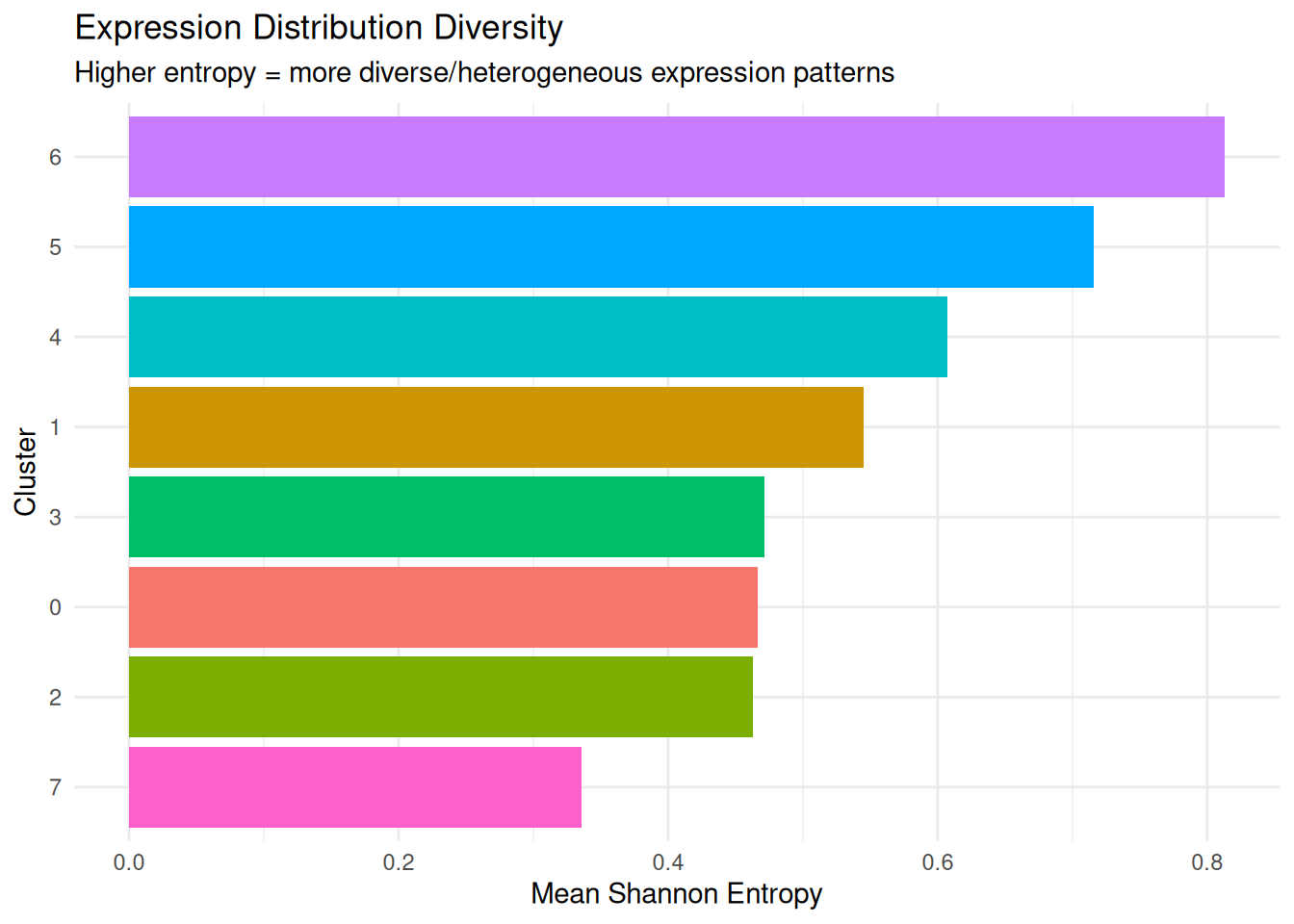
| Version | Author | Date |
|---|---|---|
| 29f3c2e | Dave Tang | 2026-01-19 |
Cluster Compactness Metrics
What it measures: How tightly packed a cluster is relative to how far it is from other clusters.
Interpretation:
- Lower compactness ratio = cluster is tight and well-separated (low heterogeneity, good clustering)
- Higher compactness ratio = cluster is spread out or close to other clusters (high heterogeneity or poor separation)
Why it matters: This metric combines within-cluster spread with between-cluster separation, giving you a sense of both heterogeneity and cluster quality.
Calculate centroid (average position) for each cluster and plot the centroids.
centroids <- do.call(rbind, lapply(unique(clusters), function(cl) {
  cells_in_cluster <- which(clusters == cl)
  colMeans(pca_embeddings[cells_in_cluster, ])
}))
rownames(centroids) <- unique(clusters)

centroids |>
  as.data.frame() |>
  dplyr::select(PC_1, PC_2) |>
  tibble::rownames_to_column('cluster') -> centroids_1_2

DimPlot(seurat_obj, reduction = 'pca') +
  geom_text(data = centroids_1_2, aes(PC_1, PC_2, label=cluster))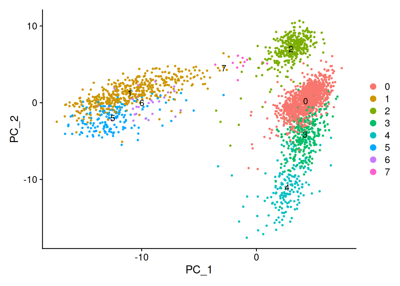
| Version | Author | Date |
|---|---|---|
| 29f3c2e | Dave Tang | 2026-01-19 |
Calculate compactness metrics for each cluster.
compactness_results <- lapply(unique(clusters), function(cl) {
  # Get cells in this cluster
  cells_in_cluster <- which(clusters == cl)
  cluster_embeddings <- pca_embeddings[cells_in_cluster, ]
  centroid <- centroids[as.character(cl), ]

  # Average distance from each cell to its cluster centroid
  distances_to_centroid <- sqrt(apply(cluster_embeddings, 1, function(x) {
    sum((x - centroid)^2)
  }))
  avg_dist_to_centroid <- mean(distances_to_centroid)

  # Find distance to nearest other cluster centroid
  other_centroids <- centroids[rownames(centroids) != as.character(cl), , drop = FALSE]
  distances_to_others <- sqrt(apply(other_centroids, 1, function(x) {
    sum((x - centroid)^2)
  }))
  min_dist_to_other <- min(distances_to_others)

  # Compactness ratio: within-cluster spread / between-cluster separation
  # Lower is better (tight cluster, well separated)
  compactness_ratio <- avg_dist_to_centroid / min_dist_to_other

  data.frame(
    cluster = cl,
    avg_dist_to_centroid = avg_dist_to_centroid,
    min_dist_to_other_cluster = min_dist_to_other,
    compactness_ratio = compactness_ratio
  )
}) |> dplyr::bind_rows()

compactness_results |>
  dplyr::arrange(compactness_ratio)
cluster avg_dist_to_centroid min_dist_to_other_cluster compactness_ratio
1 7 21.678738 50.009625 0.4334913
2 6 9.440624 15.732483 0.6000721
3 2 9.104142 11.632653 0.7826368
4 1 9.160213 11.230275 0.8156713
5 5 9.171301 11.230275 0.8166587
6 0 7.766563 7.448532 1.0426971
7 4 13.837291 11.205812 1.2348315
8 3 9.462958 7.448532 1.2704459Plot.
ggplot(compactness_results, aes(x = reorder(cluster, -compactness_ratio),
                                y = compactness_ratio, fill = cluster)) +
  geom_bar(stat = "identity") +
  coord_flip() +
  labs(title = "Cluster Compactness Ratio",
       subtitle = "Lower ratio = more compact cluster = lower heterogeneity",
       x = "Cluster", y = "Compactness Ratio") +
  theme_minimal() +
  theme(legend.position = "none")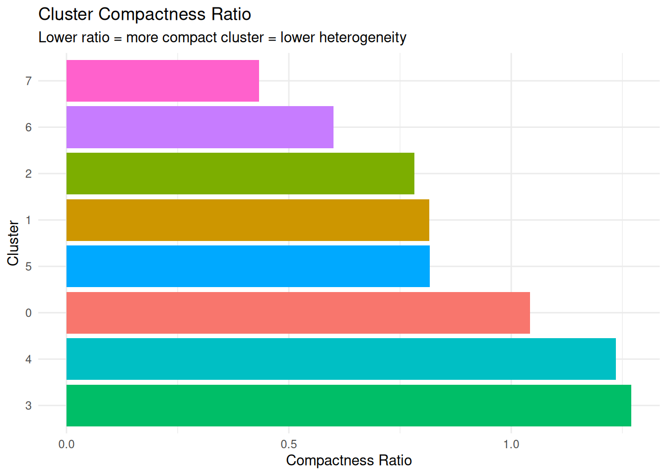
| Version | Author | Date |
|---|---|---|
| 29f3c2e | Dave Tang | 2026-01-19 |
Comparing Metrics
Combine all metrics into one table.
summary_comparison <- sil_summary |>
  dplyr::left_join(variance_results, by = "cluster") |>
  dplyr::left_join(pca_dist_summary |> dplyr::select(cluster, mean_distance),
                   by = "cluster") |>
  dplyr::left_join(entropy_results |> dplyr::select(cluster, mean_entropy),
                   by = "cluster") |>
  dplyr::left_join(compactness_results |> dplyr::select(cluster, compactness_ratio),
                   by = "cluster")

summary_comparison <- summary_comparison |>
  dplyr::select(cluster, avg_silhouette, mean_cv, mean_distance, mean_entropy, compactness_ratio)

summary_comparison
cluster avg_silhouette mean_cv mean_distance mean_entropy compactness_ratio
1 7 0.39537997 1.107976 31.91325 0.3359647 0.4334913
2 6 0.32047942 1.908411 13.63669 0.8132893 0.6000721
3 0 0.23125232 3.894674 11.06922 0.4665801 1.0426971
4 2 0.22471219 3.814635 13.05064 0.4626997 0.7826368
5 5 0.22205239 2.810056 13.06556 0.7158309 0.8166587
6 1 0.21488745 3.690295 12.98647 0.5451594 0.8156713
7 3 0.05981687 3.505332 13.44704 0.4712475 1.2704459
8 4 0.01407852 3.124803 20.08154 0.6069528 1.2348315As a heatmap.
summary_comparison |>
  tibble::column_to_rownames('cluster') |>
  as.matrix() |>
  pheatmap(scale = "column")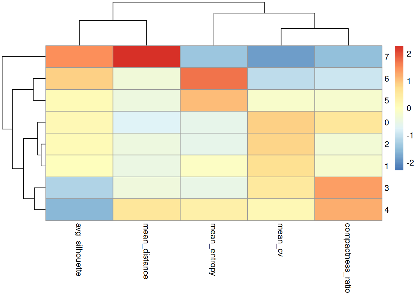
| Version | Author | Date |
|---|---|---|
| 29f3c2e | Dave Tang | 2026-01-19 |
Interpretation Guide
Each metric captures a different aspect of heterogeneity:
- Silhouette scores: Overall cluster quality and
separation
- Best for: Identifying poorly defined or overlapping clusters
- Coefficient of Variation (CV): Gene expression
variability
- Best for: Understanding transcriptional diversity within cell types
- Intra-cluster distances: Spatial spread in reduced
dimensions
- Best for: Visual/geometric sense of cluster compactness
- Shannon entropy: Distribution diversity of
expression values
- Best for: Detecting transitional states or stressed populations
- Compactness ratio: Spread relative to cluster
separation
- Best for: Combined measure of internal heterogeneity and cluster quality
sessionInfo()R version 4.5.0 (2025-04-11)
Platform: x86_64-pc-linux-gnu
Running under: Ubuntu 24.04.3 LTS
Matrix products: default
BLAS: /usr/lib/x86_64-linux-gnu/openblas-pthread/libblas.so.3
LAPACK: /usr/lib/x86_64-linux-gnu/openblas-pthread/libopenblasp-r0.3.26.so; LAPACK version 3.12.0
locale:
[1] LC_CTYPE=en_US.UTF-8 LC_NUMERIC=C
[3] LC_TIME=en_US.UTF-8 LC_COLLATE=en_US.UTF-8
[5] LC_MONETARY=en_US.UTF-8 LC_MESSAGES=en_US.UTF-8
[7] LC_PAPER=en_US.UTF-8 LC_NAME=C
[9] LC_ADDRESS=C LC_TELEPHONE=C
[11] LC_MEASUREMENT=en_US.UTF-8 LC_IDENTIFICATION=C
time zone: Etc/UTC
tzcode source: system (glibc)
attached base packages:
[1] stats graphics grDevices utils datasets methods base
other attached packages:
[1] future_1.58.0 pheatmap_1.0.13 cluster_2.1.8.1 Seurat_5.3.0
[5] SeuratObject_5.1.0 sp_2.2-0 lubridate_1.9.4 forcats_1.0.0
[9] stringr_1.5.1 dplyr_1.1.4 purrr_1.0.4 readr_2.1.5
[13] tidyr_1.3.1 tibble_3.3.0 ggplot2_3.5.2 tidyverse_2.0.0
[17] workflowr_1.7.1
loaded via a namespace (and not attached):
[1] RColorBrewer_1.1-3 rstudioapi_0.17.1 jsonlite_2.0.0
[4] magrittr_2.0.3 spatstat.utils_3.1-5 farver_2.1.2
[7] rmarkdown_2.29 fs_1.6.6 vctrs_0.6.5
[10] ROCR_1.0-11 spatstat.explore_3.5-2 htmltools_0.5.8.1
[13] sass_0.4.10 sctransform_0.4.2 parallelly_1.45.0
[16] KernSmooth_2.23-26 bslib_0.9.0 htmlwidgets_1.6.4
[19] ica_1.0-3 plyr_1.8.9 plotly_4.11.0
[22] zoo_1.8-14 cachem_1.1.0 whisker_0.4.1
[25] igraph_2.1.4 mime_0.13 lifecycle_1.0.4
[28] pkgconfig_2.0.3 Matrix_1.7-3 R6_2.6.1
[31] fastmap_1.2.0 fitdistrplus_1.2-4 shiny_1.11.1
[34] digest_0.6.37 colorspace_2.1-1 patchwork_1.3.0
[37] ps_1.9.1 rprojroot_2.0.4 tensor_1.5.1
[40] RSpectra_0.16-2 irlba_2.3.5.1 labeling_0.4.3
[43] progressr_0.15.1 spatstat.sparse_3.1-0 timechange_0.3.0
[46] httr_1.4.7 polyclip_1.10-7 abind_1.4-8
[49] compiler_4.5.0 withr_3.0.2 fastDummies_1.7.5
[52] MASS_7.3-65 tools_4.5.0 lmtest_0.9-40
[55] httpuv_1.6.16 future.apply_1.20.0 goftest_1.2-3
[58] glue_1.8.0 callr_3.7.6 nlme_3.1-168
[61] promises_1.3.3 grid_4.5.0 Rtsne_0.17
[64] getPass_0.2-4 reshape2_1.4.4 generics_0.1.4
[67] gtable_0.3.6 spatstat.data_3.1-6 tzdb_0.5.0
[70] data.table_1.17.4 hms_1.1.3 spatstat.geom_3.5-0
[73] RcppAnnoy_0.0.22 ggrepel_0.9.6 RANN_2.6.2
[76] pillar_1.10.2 spam_2.11-1 RcppHNSW_0.6.0
[79] later_1.4.2 splines_4.5.0 lattice_0.22-6
[82] survival_3.8-3 deldir_2.0-4 tidyselect_1.2.1
[85] miniUI_0.1.2 pbapply_1.7-4 knitr_1.50
[88] git2r_0.36.2 gridExtra_2.3 scattermore_1.2
[91] xfun_0.52 matrixStats_1.5.0 stringi_1.8.7
[94] lazyeval_0.2.2 yaml_2.3.10 evaluate_1.0.3
[97] codetools_0.2-20 cli_3.6.5 uwot_0.2.3
[100] xtable_1.8-4 reticulate_1.43.0 processx_3.8.6
[103] jquerylib_0.1.4 Rcpp_1.0.14 globals_0.18.0
[106] spatstat.random_3.4-1 png_0.1-8 spatstat.univar_3.1-4
[109] parallel_4.5.0 dotCall64_1.2 listenv_0.9.1
[112] viridisLite_0.4.2 scales_1.4.0 ggridges_0.5.6
[115] rlang_1.1.6 cowplot_1.2.0