Community Ecology Package
2026-01-16
Last updated: 2026-01-16
Checks: 7 0
Knit directory: muse/
This reproducible R Markdown analysis was created with workflowr (version 1.7.1). The Checks tab describes the reproducibility checks that were applied when the results were created. The Past versions tab lists the development history.
Great! Since the R Markdown file has been committed to the Git repository, you know the exact version of the code that produced these results.
Great job! The global environment was empty. Objects defined in the global environment can affect the analysis in your R Markdown file in unknown ways. For reproduciblity it’s best to always run the code in an empty environment.
The command set.seed(20200712) was run prior to running
the code in the R Markdown file. Setting a seed ensures that any results
that rely on randomness, e.g. subsampling or permutations, are
reproducible.
Great job! Recording the operating system, R version, and package versions is critical for reproducibility.
Nice! There were no cached chunks for this analysis, so you can be confident that you successfully produced the results during this run.
Great job! Using relative paths to the files within your workflowr project makes it easier to run your code on other machines.
Great! You are using Git for version control. Tracking code development and connecting the code version to the results is critical for reproducibility.
The results in this page were generated with repository version d1ab5ce. See the Past versions tab to see a history of the changes made to the R Markdown and HTML files.
Note that you need to be careful to ensure that all relevant files for
the analysis have been committed to Git prior to generating the results
(you can use wflow_publish or
wflow_git_commit). workflowr only checks the R Markdown
file, but you know if there are other scripts or data files that it
depends on. Below is the status of the Git repository when the results
were generated:
Ignored files:
    Ignored:    .Rproj.user/
    Ignored:    data/1M_neurons_filtered_gene_bc_matrices_h5.h5
    Ignored:    data/293t/
    Ignored:    data/293t_3t3_filtered_gene_bc_matrices.tar.gz
    Ignored:    data/293t_filtered_gene_bc_matrices.tar.gz
    Ignored:    data/5k_Human_Donor1_PBMC_3p_gem-x_5k_Human_Donor1_PBMC_3p_gem-x_count_sample_filtered_feature_bc_matrix.h5
    Ignored:    data/5k_Human_Donor2_PBMC_3p_gem-x_5k_Human_Donor2_PBMC_3p_gem-x_count_sample_filtered_feature_bc_matrix.h5
    Ignored:    data/5k_Human_Donor3_PBMC_3p_gem-x_5k_Human_Donor3_PBMC_3p_gem-x_count_sample_filtered_feature_bc_matrix.h5
    Ignored:    data/5k_Human_Donor4_PBMC_3p_gem-x_5k_Human_Donor4_PBMC_3p_gem-x_count_sample_filtered_feature_bc_matrix.h5
    Ignored:    data/97516b79-8d08-46a6-b329-5d0a25b0be98.h5ad
    Ignored:    data/Parent_SC3v3_Human_Glioblastoma_filtered_feature_bc_matrix.tar.gz
    Ignored:    data/brain_counts/
    Ignored:    data/cl.obo
    Ignored:    data/cl.owl
    Ignored:    data/jurkat/
    Ignored:    data/jurkat:293t_50:50_filtered_gene_bc_matrices.tar.gz
    Ignored:    data/jurkat_293t/
    Ignored:    data/jurkat_filtered_gene_bc_matrices.tar.gz
    Ignored:    data/pbmc20k/
    Ignored:    data/pbmc20k_seurat/
    Ignored:    data/pbmc3k.csv
    Ignored:    data/pbmc3k.csv.gz
    Ignored:    data/pbmc3k.h5ad
    Ignored:    data/pbmc3k/
    Ignored:    data/pbmc3k_bpcells_mat/
    Ignored:    data/pbmc3k_export.mtx
    Ignored:    data/pbmc3k_matrix.mtx
    Ignored:    data/pbmc3k_seurat.rds
    Ignored:    data/pbmc4k_filtered_gene_bc_matrices.tar.gz
    Ignored:    data/pbmc_1k_v3_filtered_feature_bc_matrix.h5
    Ignored:    data/pbmc_1k_v3_raw_feature_bc_matrix.h5
    Ignored:    data/refdata-gex-GRCh38-2020-A.tar.gz
    Ignored:    data/seurat_1m_neuron.rds
    Ignored:    data/t_3k_filtered_gene_bc_matrices.tar.gz
    Ignored:    r_packages_4.4.1/
    Ignored:    r_packages_4.5.0/

Untracked files:
    Untracked:  analysis/bioc.Rmd
    Untracked:  analysis/bioc_scrnaseq.Rmd
    Untracked:  analysis/likelihood.Rmd
    Untracked:  bpcells_matrix/
    Untracked:  data/Caenorhabditis_elegans.WBcel235.113.gtf.gz
    Untracked:  data/GCF_043380555.1-RS_2024_12_gene_ontology.gaf.gz
    Untracked:  data/arab.rds
    Untracked:  data/astronomicalunit.csv
    Untracked:  data/femaleMiceWeights.csv
    Untracked:  data/lung_bcell.rds
    Untracked:  m3/
    Untracked:  women.json

Unstaged changes:
    Modified:   analysis/isoform_switch_analyzer.Rmd
Note that any generated files, e.g. HTML, png, CSS, etc., are not included in this status report because it is ok for generated content to have uncommitted changes.
These are the previous versions of the repository in which changes were
made to the R Markdown (analysis/vegan.Rmd) and HTML
(docs/vegan.html) files. If you’ve configured a remote Git
repository (see ?wflow_git_remote), click on the hyperlinks
in the table below to view the files as they were in that past version.
| File | Version | Author | Date | Message |
|---|---|---|---|---|
| Rmd | d1ab5ce | Dave Tang | 2026-01-16 | Similarity versus dissimilarity |
| html | 0195105 | Dave Tang | 2025-09-09 | Build site. |
| Rmd | b54e12a | Dave Tang | 2025-09-09 | Horn-Morisita index |
Introduction
The {vegan} package contains “Ordination methods, diversity analysis and other functions for community and vegetation ecologists.”
Setup
Install {vegan}.
install.packages("vegan")
install.packages("ggdendro")
Dissimilarity indices
?vegdist:
The function computes dissimilarity indices that are useful for or popular with community ecologists. All indices use quantitative data, although they would be named by the corresponding binary index, but you can calculate the binary index using an appropriate argument. If you do not find your favourite index here, you can see if it can be implemented using designdist. Gower, Bray–Curtis, Jaccard and Kulczynski indices are good in detecting underlying ecological gradients (Faith et al. 1987). Morisita, Horn–Morisita, Binomial, Cao and Chao indices should be able to handle different sample sizes (Wolda 1981, Krebs 1999, Anderson & Millar 2004), and Mountford (1962) and Raup-Crick indices for presence–absence data should be able to handle unknown (and variable) sample sizes. Most of these indices are discussed by Krebs (1999) and Legendre & Legendre (2012), and their properties further compared by Wolda (1981) and Legendre & De Cáceres (2012). Aitchison (1986) distance is equivalent to Euclidean distance between CLR-transformed samples (“clr”) and deals with positive compositional data. Robust Aitchison distance by Martino et al. (2019) uses robust CLR (“rlcr”), making it applicable to non-negative data including zeroes (unlike the standard Aitchison).
Methods include: “manhattan”, “euclidean”, “canberra”, “clark”, “bray”, “kulczynski”, “jaccard”, “gower”, “altGower”, “morisita”, “horn”, “mountford”, “raup”, “binomial”, “chao”, “cao”, “mahalanobis”, “chisq”, “chord”, “hellinger”, “aitchison”, or “robust.aitchison”.
Morisita index can be used with genuine count data (integers) only. Its Horn–Morisita variant is able to handle any abundance data.
The abbreviation “horn” for the Horn–Morisita index is misleading, since there is a separate Horn index. The abbreviation will be changed if that index is implemented in vegan.
?varespec:
- The varespec data frame has 24 rows and 44 columns.
- Columns are estimated cover values of 44 species.
- Rows are sites.
- The variable names are formed from the scientific names, and are self explanatory for anybody familiar with the vegetation type.
data(varespec)
varespec[1:6, 1:6]
Callvulg Empenigr Rhodtome Vaccmyrt Vaccviti Pinusylv
18 0.55 11.13 0.00 0.00 17.80 0.07
15 0.67 0.17 0.00 0.35 12.13 0.12
24 0.10 1.55 0.00 0.00 13.47 0.25
27 0.00 15.13 2.42 5.92 15.97 0.00
23 0.00 12.68 0.00 0.00 23.73 0.03
19 0.00 8.92 0.00 2.42 10.28 0.12Horn-Morisita dissimilarity indices for the first six sites.
vegdist(varespec[1:6, ], method = "horn") 18 15 24 27 23
15 0.4886065
24 0.6343112 0.2090845
27 0.6154254 0.0975100 0.2172843
23 0.2220906 0.2213285 0.3352133 0.2380449
19 0.4465064 0.3084495 0.4119088 0.2656402 0.2935237Note that:
- Diversity indices measure variation within a single sample.
- Similarity (and dissimilarity) indices measure how alike or different two samples are.
Example data
Count matrix.
set.seed(1984)

cell_types <- c(
  "Neural Progenitors",
  "Neurons",
  "Astrocytes",
  "Oligodendrocytes",
  "Microglia",
  "Endothelial",
  "Radial Glia",
  "Intermediate Progenitors"
)

count_matrix <- base::matrix(c(
  450, 480, 420, 380, 350, 340, 400, 380,
  200, 800, 150, 120, 80, 100, 250, 200,
  100, 1200, 50, 30, 20, 40, 80, 60,
  500, 300, 250, 200, 150, 100, 80, 50,
  300, 500, 200, 180, 150, 120, 200, 150
), nrow = 8, ncol = 5, byrow = FALSE)
count_matrix
[,1] [,2] [,3] [,4] [,5]
[1,] 450 200 100 500 300
[2,] 480 800 1200 300 500
[3,] 420 150 50 250 200
[4,] 380 120 30 200 180
[5,] 350 80 20 150 150
[6,] 340 100 40 100 120
[7,] 400 250 80 80 200
[8,] 380 200 60 50 150base::rownames(count_matrix) <- cell_types
base::colnames(count_matrix) <- letters[1:ncol(count_matrix)]
count_matrix a b c d e
Neural Progenitors 450 200 100 500 300
Neurons 480 800 1200 300 500
Astrocytes 420 150 50 250 200
Oligodendrocytes 380 120 30 200 180
Microglia 350 80 20 150 150
Endothelial 340 100 40 100 120
Radial Glia 400 250 80 80 200
Intermediate Progenitors 380 200 60 50 150Similarity versus dissimilarity
- Similarity indices range from 0 (completely different) to 1 (identical)
- Dissimilarity/Distance indices range from 0 (identical) to higher values (more different)
Conversion: Dissimilarity = 1 - Similarity (for indices scaled 0-1)
Bray-Curtis Dissimilarity
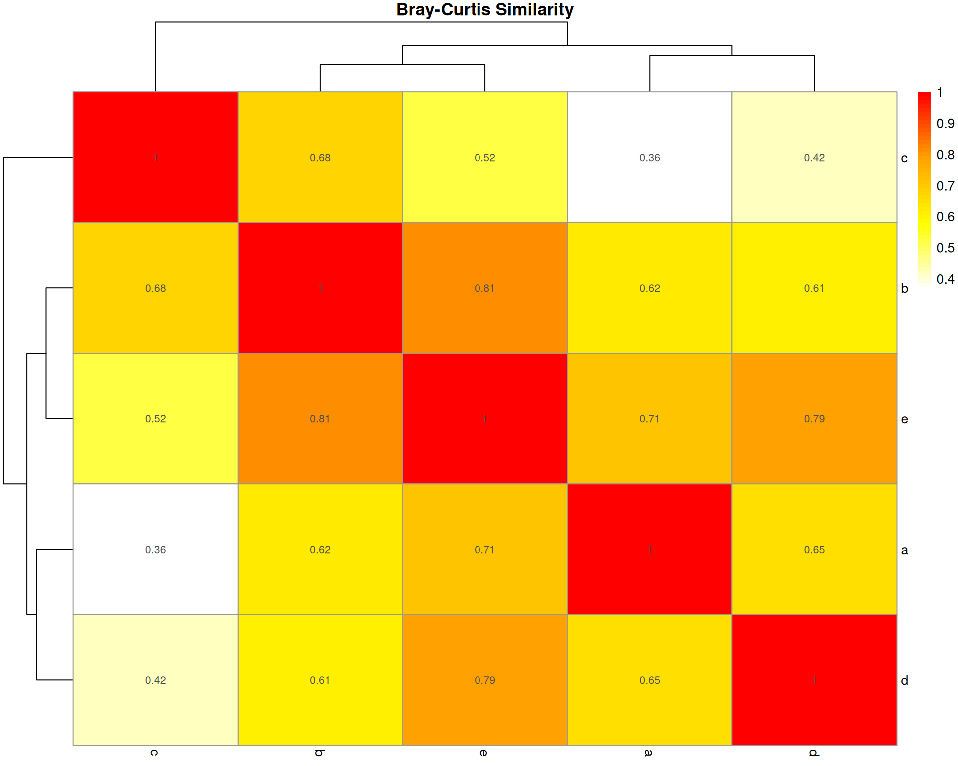
What it measures: The absolute difference in cell type abundances between two organoids, normalised by total abundance.
Interpretation: * Ranges from 0 (identical) to 1 (completely different) * 0.3-0.5 often considered moderately similar * Sensitive to both presence/absence and abundance differences
Key characteristic: Most widely used in ecology; emphasises absolute differences in abundances. Does NOT account for sampling effects.
bray_dist <- vegan::vegdist(base::t(count_matrix), method = "bray")
bray_matrix <- base::as.matrix(bray_dist)
bray_similarity <- 1 - bray_matrix
bray_similarity
a b c d e
a 1.0000000 0.6196078 0.3598326 0.6542443 0.7120000
b 0.6196078 1.0000000 0.6781609 0.6118980 0.8108108
c 0.3598326 0.6781609 1.0000000 0.4174455 0.5207101
d 0.6542443 0.6118980 0.4174455 1.0000000 0.7930029
e 0.7120000 0.8108108 0.5207101 0.7930029 1.0000000pheatmap::pheatmap(
bray_similarity,
cluster_rows = TRUE,
cluster_cols = TRUE,
display_numbers = base::round(bray_similarity, 2),
main = "Bray-Curtis Similarity",
color = grDevices::colorRampPalette(c("white", "yellow", "orange", "red"))(50)
)
Horn-Morisita Index
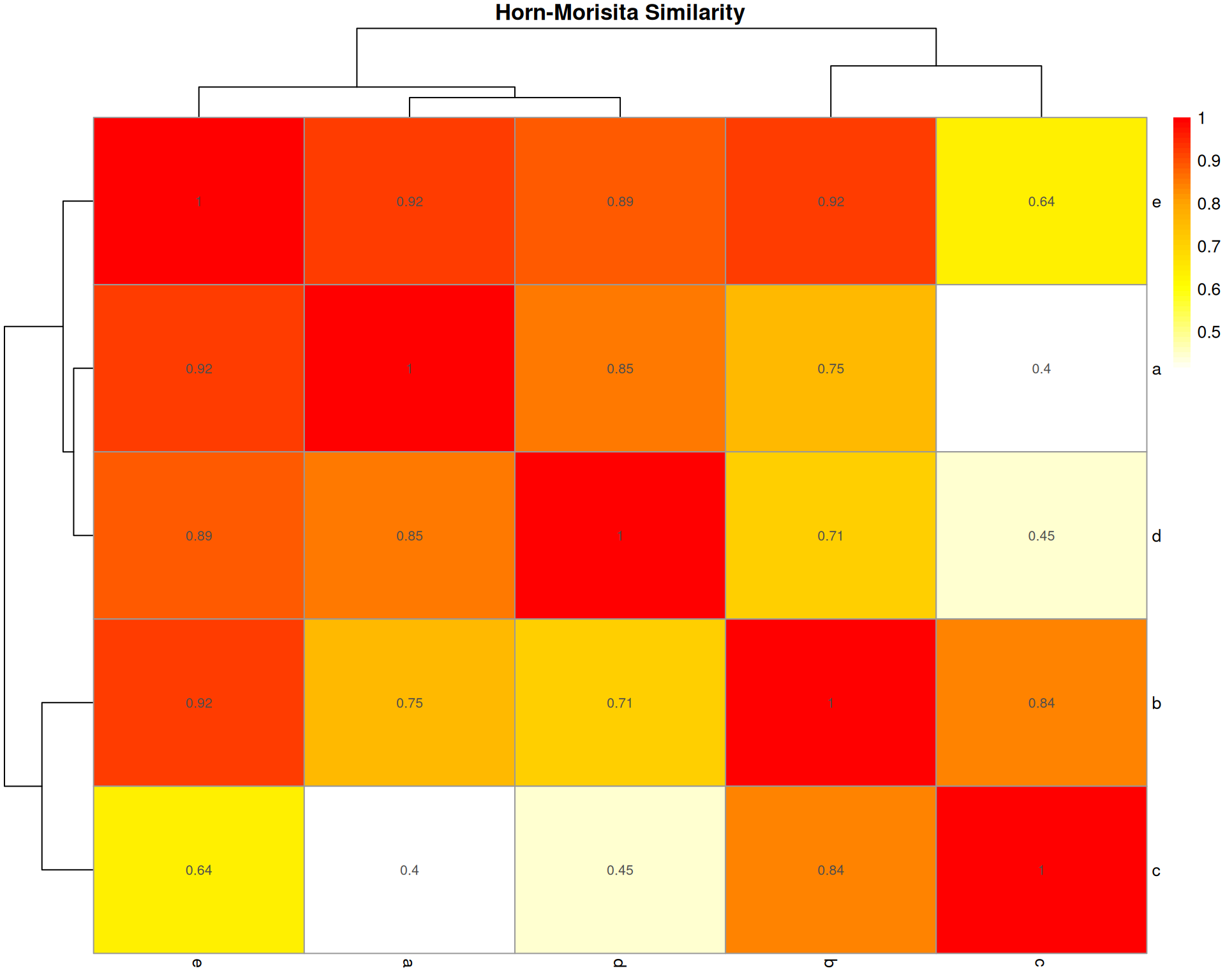
What it measures: The probability that two randomly selected cells (one from each organoid) belong to the same cell type.
Formula: Based on Morisita’s index but modified by Horn to be independent of sample size and species diversity.
Interpretation: * Ranges from 0 (no overlap) to 1 (identical composition) * > 0.6 typically indicates high similarity * > 0.75 indicates very high similarity
Key characteristic: Robust to differences in sample size. Less affected by species richness than Bray-Curtis. Better for comparing samples with different total abundances.
horn_dist <- vegan::vegdist(base::t(count_matrix), method = "horn")
horn_matrix <- base::as.matrix(horn_dist)
horn_similarity <- 1 - horn_matrix

pheatmap::pheatmap(
  horn_similarity,
  cluster_rows = TRUE,
  cluster_cols = TRUE,
  display_numbers = base::round(horn_similarity, 2),
  main = "Horn-Morisita Similarity",
  color = grDevices::colorRampPalette(c("white", "yellow", "orange", "red"))(50)
)
Euclidean Distance
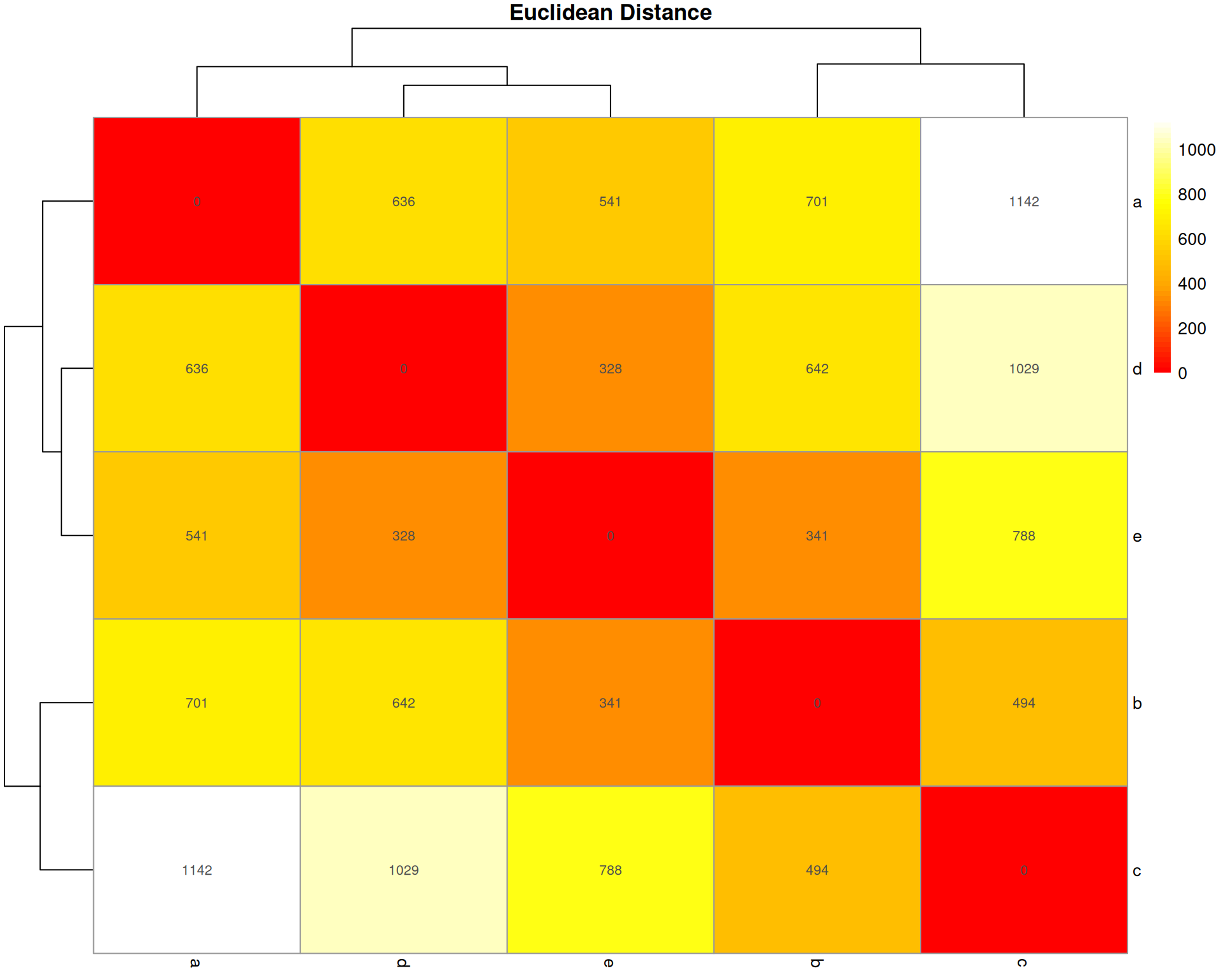
What it measures: The straight-line distance between two organoids in multidimensional space (one dimension per cell type).
Interpretation: * Ranges from 0 (identical) to infinity * Larger values = more different * No upper bound (not scaled to 1)
Key characteristic: Sensitive to total abundance and scale. Square root of sum of squared differences. Common in general clustering but less ideal for compositional data.
euclidean_dist <- stats::dist(base::t(count_matrix), method = "euclidean")
euclidean_matrix <- base::as.matrix(euclidean_dist)

pheatmap::pheatmap(
  euclidean_matrix,
  cluster_rows = TRUE,
  cluster_cols = TRUE,
  display_numbers = base::round(euclidean_matrix, 0),
  main = "Euclidean Distance",
  color = grDevices::colorRampPalette(c("red", "orange", "yellow", "white"))(50)
)
sessionInfo()R version 4.5.0 (2025-04-11)
Platform: x86_64-pc-linux-gnu
Running under: Ubuntu 24.04.3 LTS
Matrix products: default
BLAS: /usr/lib/x86_64-linux-gnu/openblas-pthread/libblas.so.3
LAPACK: /usr/lib/x86_64-linux-gnu/openblas-pthread/libopenblasp-r0.3.26.so; LAPACK version 3.12.0
locale:
[1] LC_CTYPE=en_US.UTF-8 LC_NUMERIC=C
[3] LC_TIME=en_US.UTF-8 LC_COLLATE=en_US.UTF-8
[5] LC_MONETARY=en_US.UTF-8 LC_MESSAGES=en_US.UTF-8
[7] LC_PAPER=en_US.UTF-8 LC_NAME=C
[9] LC_ADDRESS=C LC_TELEPHONE=C
[11] LC_MEASUREMENT=en_US.UTF-8 LC_IDENTIFICATION=C
time zone: Etc/UTC
tzcode source: system (glibc)
attached base packages:
[1] stats graphics grDevices utils datasets methods base
other attached packages:
[1] ggdendro_0.2.0 vegan_2.7-1 permute_0.9-8 lubridate_1.9.4
[5] forcats_1.0.0 stringr_1.5.1 dplyr_1.1.4 purrr_1.0.4
[9] readr_2.1.5 tidyr_1.3.1 tibble_3.3.0 ggplot2_3.5.2
[13] tidyverse_2.0.0 workflowr_1.7.1
loaded via a namespace (and not attached):
[1] gtable_0.3.6 xfun_0.52 bslib_0.9.0 processx_3.8.6
[5] lattice_0.22-6 callr_3.7.6 tzdb_0.5.0 vctrs_0.6.5
[9] tools_4.5.0 ps_1.9.1 generics_0.1.4 parallel_4.5.0
[13] cluster_2.1.8.1 pkgconfig_2.0.3 pheatmap_1.0.13 Matrix_1.7-3
[17] RColorBrewer_1.1-3 lifecycle_1.0.4 compiler_4.5.0 farver_2.1.2
[21] git2r_0.36.2 getPass_0.2-4 httpuv_1.6.16 htmltools_0.5.8.1
[25] sass_0.4.10 yaml_2.3.10 later_1.4.2 pillar_1.10.2
[29] jquerylib_0.1.4 whisker_0.4.1 MASS_7.3-65 cachem_1.1.0
[33] nlme_3.1-168 tidyselect_1.2.1 digest_0.6.37 stringi_1.8.7
[37] splines_4.5.0 rprojroot_2.0.4 fastmap_1.2.0 grid_4.5.0
[41] cli_3.6.5 magrittr_2.0.3 withr_3.0.2 scales_1.4.0
[45] promises_1.3.3 timechange_0.3.0 rmarkdown_2.29 httr_1.4.7
[49] hms_1.1.3 evaluate_1.0.3 knitr_1.50 mgcv_1.9-1
[53] rlang_1.1.6 Rcpp_1.0.14 glue_1.8.0 rstudioapi_0.17.1
[57] jsonlite_2.0.0 R6_2.6.1 fs_1.6.6