Gene Ontology Enrichment Analysis
2021-01-30
Last updated: 2021-01-30
Checks: 7 0
Knit directory: muse/
This reproducible R Markdown analysis was created with workflowr (version 1.6.2). The Checks tab describes the reproducibility checks that were applied when the results were created. The Past versions tab lists the development history.
Great! Since the R Markdown file has been committed to the Git repository, you know the exact version of the code that produced these results.
Great job! The global environment was empty. Objects defined in the global environment can affect the analysis in your R Markdown file in unknown ways. For reproduciblity it’s best to always run the code in an empty environment.
The command set.seed(20200712) was run prior to running the code in the R Markdown file. Setting a seed ensures that any results that rely on randomness, e.g. subsampling or permutations, are reproducible.
Great job! Recording the operating system, R version, and package versions is critical for reproducibility.
Nice! There were no cached chunks for this analysis, so you can be confident that you successfully produced the results during this run.
Great job! Using relative paths to the files within your workflowr project makes it easier to run your code on other machines.
Great! You are using Git for version control. Tracking code development and connecting the code version to the results is critical for reproducibility.
The results in this page were generated with repository version 909d437. See the Past versions tab to see a history of the changes made to the R Markdown and HTML files.
Note that you need to be careful to ensure that all relevant files for the analysis have been committed to Git prior to generating the results (you can use wflow_publish or wflow_git_commit). workflowr only checks the R Markdown file, but you know if there are other scripts or data files that it depends on. Below is the status of the Git repository when the results were generated:
Ignored files:
    Ignored:    .DS_Store
    Ignored:    .Rhistory
    Ignored:    .Rproj.user/
    Ignored:    analysis/.Rhistory

Untracked files:
    Untracked:  analysis/cluster_profiler.Rmd
    Untracked:  analysis/linear_regression.Rmd
    Untracked:  data/gencode.v36.annotation.gtf.gz
Note that any generated files, e.g. HTML, png, CSS, etc., are not included in this status report because it is ok for generated content to have uncommitted changes.
These are the previous versions of the repository in which changes were made to the R Markdown (analysis/go_enrichment.Rmd) and HTML (docs/go_enrichment.html) files. If you’ve configured a remote Git repository (see ?wflow_git_remote), click on the hyperlinks in the table below to view the files as they were in that past version.
| File | Version | Author | Date | Message |
|---|---|---|---|---|
| Rmd | 909d437 | davetang | 2021-01-30 | compareCluster function |
| html | 22ec290 | davetang | 2021-01-28 | Build site. |
| Rmd | 9cf163e | davetang | 2021-01-28 | GO primer and included visualisations |
| html | 795f0f4 | davetang | 2021-01-27 | Build site. |
| Rmd | 3c146e5 | davetang | 2021-01-27 | Include clusterProfiler |
| html | 1cd1577 | davetang | 2021-01-27 | Build site. |
| Rmd | 687a6ca | davetang | 2021-01-27 | Gene Ontology Enrichment Analysis |
Getting started
The Gene Ontology Enrichment Analysis (GOEA) is a typical analysis carried out on transcriptome data. Online tools for performing a GOEA include DAVID, Enrichr, and PANTHER just to name a few. While web-based tools are easy to use, it becomes tedious when you have to analyse (or re-analyse) lots of datasets. Therefore, it is preferable to use a programmatic approach and in this post we will check out some Bioconductor packages that allow to perform a GOEA.
First install the following packages, if necessary, and then load them.
if (!requireNamespace("BiocManager", quietly = TRUE))
    install.packages("BiocManager")

my_packages <- c("clusterProfiler",
                 "GOstats",
                 "GO.db",
                 "org.Hs.eg.db")

to_install <- my_packages[!my_packages %in% installed.packages()]

# install missing packages, if any
if (length(to_install) > 0){
  BiocManager::install(pkgs = to_install)
}

# load all packages and suppress output of sapply
invisible(sapply(my_packages, library, character.only = TRUE))
Create a positive control where the gene set are composed of genes that are all associated with GO:0007411 (axon guidance); we will use the org.Hs.eg.db package to achieve this based on the vignette.
Methods that can be applied to AnnotationDbi objects such as org.Hs.eg.db include: columns, keytypes, keys, and select.
Use columns to find out what data can be retrived using select.
columns(org.Hs.eg.db) [1] "ACCNUM" "ALIAS" "ENSEMBL" "ENSEMBLPROT" "ENSEMBLTRANS"
[6] "ENTREZID" "ENZYME" "EVIDENCE" "EVIDENCEALL" "GENENAME"
[11] "GO" "GOALL" "IPI" "MAP" "OMIM"
[16] "ONTOLOGY" "ONTOLOGYALL" "PATH" "PFAM" "PMID"
[21] "PROSITE" "REFSEQ" "SYMBOL" "UCSCKG" "UNIGENE"
[26] "UNIPROT" Use keytypes to find out what fields we can use as keys to query the database.
keytypes(org.Hs.eg.db) [1] "ACCNUM" "ALIAS" "ENSEMBL" "ENSEMBLPROT" "ENSEMBLTRANS"
[6] "ENTREZID" "ENZYME" "EVIDENCE" "EVIDENCEALL" "GENENAME"
[11] "GO" "GOALL" "IPI" "MAP" "OMIM"
[16] "ONTOLOGY" "ONTOLOGYALL" "PATH" "PFAM" "PMID"
[21] "PROSITE" "REFSEQ" "SYMBOL" "UCSCKG" "UNIGENE"
[26] "UNIPROT" Select all genes with GO:0007411.
go_to_entrez <- select(org.Hs.eg.db,
                       keys = "GO:0007411",
                       columns = "ENTREZID",
                       keytype = "GO")
'select()' returned 1:many mapping between keys and columnsaxon_gene <- unique(go_to_entrez$ENTREZID)
length(axon_gene)[1] 205Note that we can also use select on GO.db to fetch more information on GO:0007411.
select(GO.db,
       keys = "GO:0007411",
       columns = columns(GO.db),
       keytype = "GOID")
'select()' returned 1:1 mapping between keys and columns GOID
1 GO:0007411
DEFINITION
1 The chemotaxis process that directs the migration of an axon growth cone to a specific target site in response to a combination of attractive and repulsive cues.
ONTOLOGY TERM
1 BP axon guidanceTo perform the GOEA we need to create a gene background called the universe and we will use all genes with a GO term. Normally the universe should be the list of genes that were actually assayed in your transcriptome analysis.
all_go_terms <- keys(org.Hs.eg.db, keytype = "GO")
all_go <- select(org.Hs.eg.db, keys = all_go_terms, columns = c("ENTREZID", "GO"), keytype = "GO")
'select()' returned 1:many mapping between keys and columnsuniverse <- unique(all_go$ENTREZID)
length(universe)[1] 20488The function hyperGTest will perform the GOEA based on a set of parameters; in this example, we are testing for the over-representation of biological process (BP) terms and using a p-value cutoff of 0.001 or less.
params <- new('GOHyperGParams',
              geneIds = axon_gene,
              universeGeneIds = universe,
              ontology = 'BP',
              pvalueCutoff = 0.001,
              conditional = FALSE,
              testDirection = 'over',
              annotation = "org.Hs.eg.db"
             )

my_test <- hyperGTest(params)
my_test
Gene to GO BP test for over-representation
4723 GO BP ids tested (1069 have p < 0.001)
Selected gene set size: 205
Gene universe size: 18670
Annotation package: org.Hs.eg Use summary to get a summary of the results. The summary contains the GOID, Pvalue, OddsRatio, ExpCount, Count, and Size.
ExpCountis the expected countCountis how many instances of that term were actually observed in your gene listSizeis the number that could have been found in your gene list if every instance had turned up
head(summary(my_test)) GOBPID Pvalue OddsRatio ExpCount Count Size
1 GO:0007409 0.00000e+00 Inf 5.138725 205 468
2 GO:0007411 0.00000e+00 Inf 3.030530 205 276
3 GO:0048667 0.00000e+00 Inf 6.401446 205 583
4 GO:0061564 0.00000e+00 Inf 5.643814 205 514
5 GO:0097485 0.00000e+00 Inf 3.041510 205 277
6 GO:0006935 6.87054e-316 Inf 7.071237 205 644
Term
1 axonogenesis
2 axon guidance
3 cell morphogenesis involved in neuron differentiation
4 axon development
5 neuron projection guidance
6 chemotaxisGO terms associated to axons are enriched as expected. Note that the Count and Size for GO:0007411 is not identical even though we had selected all genes associated with GO:0007411. If we manually select Entrez gene IDs using org.Hs.egGO, we still get the same list of genes.
my_df <- as.data.frame(org.Hs.egGO)
my_idx <- my_df$go_id == "GO:0007411"
length(unique(my_df[my_idx, "gene_id"])) == length(axon_gene)
[1] TRUEThis is probably because genes containing GO terms that are descendants of GO:0007411 are also included.
Relations in the Gene Ontology
Gene ontologies (GO) are structured as a directed acyclic graph with GO terms as nodes and their relationships as edges. The most commonly used relationships in GO are:
- is a
- part of
- has part
- regulates
- negatively regulates
- positively regulates
Below is an example of the is a and part of relationships.

We can use the GOBPCHILDREN annotation map or Bimap from the GO.db package to retrieve all descendants of GO:0007411.
bp_children <- as.list(GOBPCHILDREN)
bp_children[["GO:0007411"]]
isa part of isa
"GO:0008045" "GO:0016198" "GO:0021966"
isa isa isa
"GO:0021967" "GO:0021968" "GO:0021969"
isa isa isa
"GO:0021970" "GO:0021971" "GO:0021972"
isa isa isa
"GO:0031290" "GO:0033563" "GO:0033564"
isa isa part of
"GO:0036514" "GO:0036515" "GO:0048846"
part of part of isa
"GO:0061642" "GO:0061643" "GO:0071678"
isa isa isa
"GO:0071679" "GO:0072499" "GO:0097374"
isa isa part of
"GO:0097376" "GO:0097492" "GO:1902287"
part of regulates negatively regulates
"GO:1902378" "GO:1902667" "GO:1902668"
positively regulates part of part of
"GO:1902669" "GO:1904938" "GO:2001266" We can include these GO terms in our select query.
my_keys <- c("GO:0007411", bp_children[["GO:0007411"]])

go_to_entrez_children <- select(org.Hs.eg.db,
                                keys = my_keys,
                                columns = "ENTREZID",
                                keytype = "GO")
'select()' returned 1:many mapping between keys and columnslength(unique(go_to_entrez_children$ENTREZID))[1] 261We are still missing some genes that are associated with GO:0007411, which is probably due to the exclusion of descendants in the descendants of GO:0007411. We need to recursively search all terms that are descendants of GO:0007411.
params <- new('GOHyperGParams',
              geneIds = unique(go_to_entrez_children$ENTREZID),
              universeGeneIds = universe,
              ontology = 'BP',
              pvalueCutoff = 0.001,
              conditional = FALSE,
              testDirection = 'over',
              annotation = "org.Hs.eg.db"
             )
Warning in makeValidParams(.Object): removing geneIds not in universeGeneIdsmy_test2 <- hyperGTest(params)
head(summary(my_test2)) GOBPID Pvalue OddsRatio ExpCount Count Size
1 GO:0000902 0 Inf 14.399572 260 1034
2 GO:0000904 0 Inf 10.361007 260 744
3 GO:0006935 0 Inf 8.968399 260 644
4 GO:0007409 0 Inf 6.517408 260 468
5 GO:0007411 0 Inf 3.843599 260 276
6 GO:0031175 0 Inf 13.619711 260 978
Term
1 cell morphogenesis
2 cell morphogenesis involved in differentiation
3 chemotaxis
4 axonogenesis
5 axon guidance
6 neuron projection developmentclusterProfiler
The enrichGO function in the clusterProfiler package can also perform a GOEA with FDR control.
my_test3 <- enrichGO(axon_gene,
                     org.Hs.eg.db,
                     keyType = "ENTREZID",
                     ont = "BP",
                     pvalueCutoff = 0.001,
                     pAdjustMethod = "BH",
                     universe,
                     qvalueCutoff = 0.1,
                     minGSSize = 10,
                     maxGSSize = 500,
                     readable = FALSE)

head(data.frame(my_test3))
ID Description GeneRatio
GO:0007409 GO:0007409 axonogenesis 205/205
GO:0007411 GO:0007411 axon guidance 205/205
GO:0097485 GO:0097485 neuron projection guidance 205/205
GO:0050770 GO:0050770 regulation of axonogenesis 41/205
GO:0008038 GO:0008038 neuron recognition 27/205
GO:0010975 GO:0010975 regulation of neuron projection development 56/205
BgRatio pvalue p.adjust qvalue
GO:0007409 468/18670 0.000000e+00 0.000000e+00 0.000000e+00
GO:0007411 276/18670 0.000000e+00 0.000000e+00 0.000000e+00
GO:0097485 277/18670 0.000000e+00 0.000000e+00 0.000000e+00
GO:0050770 183/18670 2.592496e-42 2.143346e-39 1.300341e-39
GO:0008038 48/18670 3.898825e-41 2.578683e-38 1.564455e-38
GO:0010975 499/18670 1.042084e-40 5.743620e-38 3.484583e-38
geneID
GO:0007409 323/474/627/655/682/1002/1400/1436/1600/1630/1796/1808/1826/1855/1942/1943/1944/1945/1946/1947/1948/1949/1969/2041/2042/2043/2044/2045/2046/2047/2048/2049/2050/2051/2115/2131/2297/2534/2549/2625/2637/2668/2674/2675/2676/2736/2737/2817/2885/2886/2887/2909/3730/3798/3800/3897/3908/3913/4009/4089/4147/4628/4684/4756/4902/4914/4917/4983/5015/5080/5290/5291/5293/5295/5335/5458/5578/5588/5594/5595/5598/5623/5649/5747/5781/5786/5800/5818/5909/5979/6091/6092/6259/6324/6387/6405/6464/6469/6477/6585/6586/6654/6708/6709/6710/6711/6712/6714/6900/7080/7143/7204/7408/7430/7436/7473/7474/7852/7869/8013/8399/8609/8633/8660/8828/8829/8851/9046/9048/9211/9252/9260/9353/9355/9369/9378/9499/9637/9638/9846/10048/10371/10381/10500/10505/10512/10678/10752/10818/11023/11127/11313/23022/23032/23114/23191/23767/23768/26999/27020/27255/30011/51332/51466/53358/54538/55715/55740/55816/56896/57408/57453/57549/57556/57731/59277/59352/64096/64221/64855/84665/85358/89780/90249/91624/91653/128434/133418/137970/151449/152330/170302/219699/220164/223117/283297/284217/284656/285220/374946/375790/389549/644168/654429/729920
GO:0007411 323/474/627/655/682/1002/1400/1436/1600/1630/1796/1808/1826/1855/1942/1943/1944/1945/1946/1947/1948/1949/1969/2041/2042/2043/2044/2045/2046/2047/2048/2049/2050/2051/2115/2131/2297/2534/2549/2625/2637/2668/2674/2675/2676/2736/2737/2817/2885/2886/2887/2909/3730/3798/3800/3897/3908/3913/4009/4089/4147/4628/4684/4756/4902/4914/4917/4983/5015/5080/5290/5291/5293/5295/5335/5458/5578/5588/5594/5595/5598/5623/5649/5747/5781/5786/5800/5818/5909/5979/6091/6092/6259/6324/6387/6405/6464/6469/6477/6585/6586/6654/6708/6709/6710/6711/6712/6714/6900/7080/7143/7204/7408/7430/7436/7473/7474/7852/7869/8013/8399/8609/8633/8660/8828/8829/8851/9046/9048/9211/9252/9260/9353/9355/9369/9378/9499/9637/9638/9846/10048/10371/10381/10500/10505/10512/10678/10752/10818/11023/11127/11313/23022/23032/23114/23191/23767/23768/26999/27020/27255/30011/51332/51466/53358/54538/55715/55740/55816/56896/57408/57453/57549/57556/57731/59277/59352/64096/64221/64855/84665/85358/89780/90249/91624/91653/128434/133418/137970/151449/152330/170302/219699/220164/223117/283297/284217/284656/285220/374946/375790/389549/644168/654429/729920
GO:0097485 323/474/627/655/682/1002/1400/1436/1600/1630/1796/1808/1826/1855/1942/1943/1944/1945/1946/1947/1948/1949/1969/2041/2042/2043/2044/2045/2046/2047/2048/2049/2050/2051/2115/2131/2297/2534/2549/2625/2637/2668/2674/2675/2676/2736/2737/2817/2885/2886/2887/2909/3730/3798/3800/3897/3908/3913/4009/4089/4147/4628/4684/4756/4902/4914/4917/4983/5015/5080/5290/5291/5293/5295/5335/5458/5578/5588/5594/5595/5598/5623/5649/5747/5781/5786/5800/5818/5909/5979/6091/6092/6259/6324/6387/6405/6464/6469/6477/6585/6586/6654/6708/6709/6710/6711/6712/6714/6900/7080/7143/7204/7408/7430/7436/7473/7474/7852/7869/8013/8399/8609/8633/8660/8828/8829/8851/9046/9048/9211/9252/9260/9353/9355/9369/9378/9499/9637/9638/9846/10048/10371/10381/10500/10505/10512/10678/10752/10818/11023/11127/11313/23022/23032/23114/23191/23767/23768/26999/27020/27255/30011/51332/51466/53358/54538/55715/55740/55816/56896/57408/57453/57549/57556/57731/59277/59352/64096/64221/64855/84665/85358/89780/90249/91624/91653/128434/133418/137970/151449/152330/170302/219699/220164/223117/283297/284217/284656/285220/374946/375790/389549/644168/654429/729920
GO:0050770 627/1002/1600/1630/1808/1826/1942/1946/1949/2043/2045/2048/2049/2909/3897/5458/5747/5800/5979/6091/6092/6259/6387/6405/6900/7143/7473/7474/7869/8829/8851/9353/10371/10500/10505/10512/23191/57556/89780/223117/374946
GO:0008038 682/1826/1949/2042/2043/2048/2049/2909/6091/6092/6900/7852/8829/8851/10371/23022/27020/27255/54538/57453/57549/64221/84665/91624/128434/133418/152330
GO:0010975 627/655/1002/1400/1600/1630/1808/1826/1855/1942/1946/1948/1949/2042/2043/2045/2048/2049/2534/2625/2909/3897/4914/5458/5649/5747/5800/5979/6091/6092/6259/6324/6387/6405/6900/7143/7436/7473/7474/7852/7869/8829/8851/9353/9638/10371/10500/10505/10512/23191/27020/57556/85358/89780/223117/374946
Count
GO:0007409 205
GO:0007411 205
GO:0097485 205
GO:0050770 41
GO:0008038 27
GO:0010975 56The output now includes adjusted p-values and the geneIDs that are associated with a given GO ID. Note that the full list of genes for GO:0007411 is 276 again.
In addition to performing the GOEA, clusterProfiler also has some nice plotting functions.
Bar plot showing each enriched GO term coloured by the adjusted p-value.
barplot(my_test3, showCategory=10)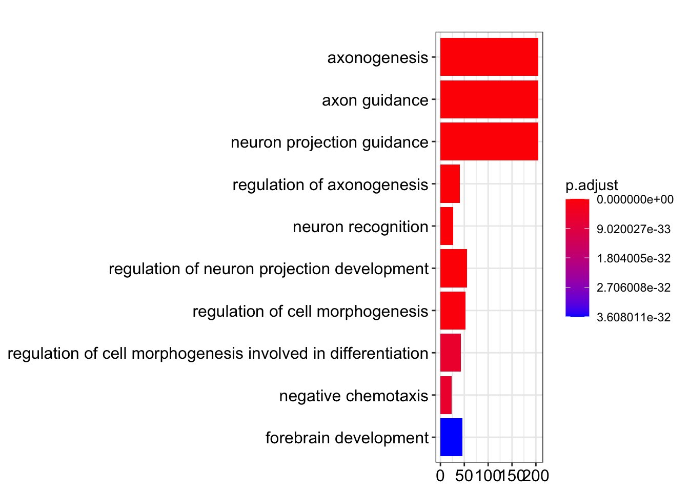
| Version | Author | Date |
|---|---|---|
| 22ec290 | davetang | 2021-01-28 |
Dot plot showing each enriched GO term with associated statistics.
dotplot(my_test3, showCategory=10)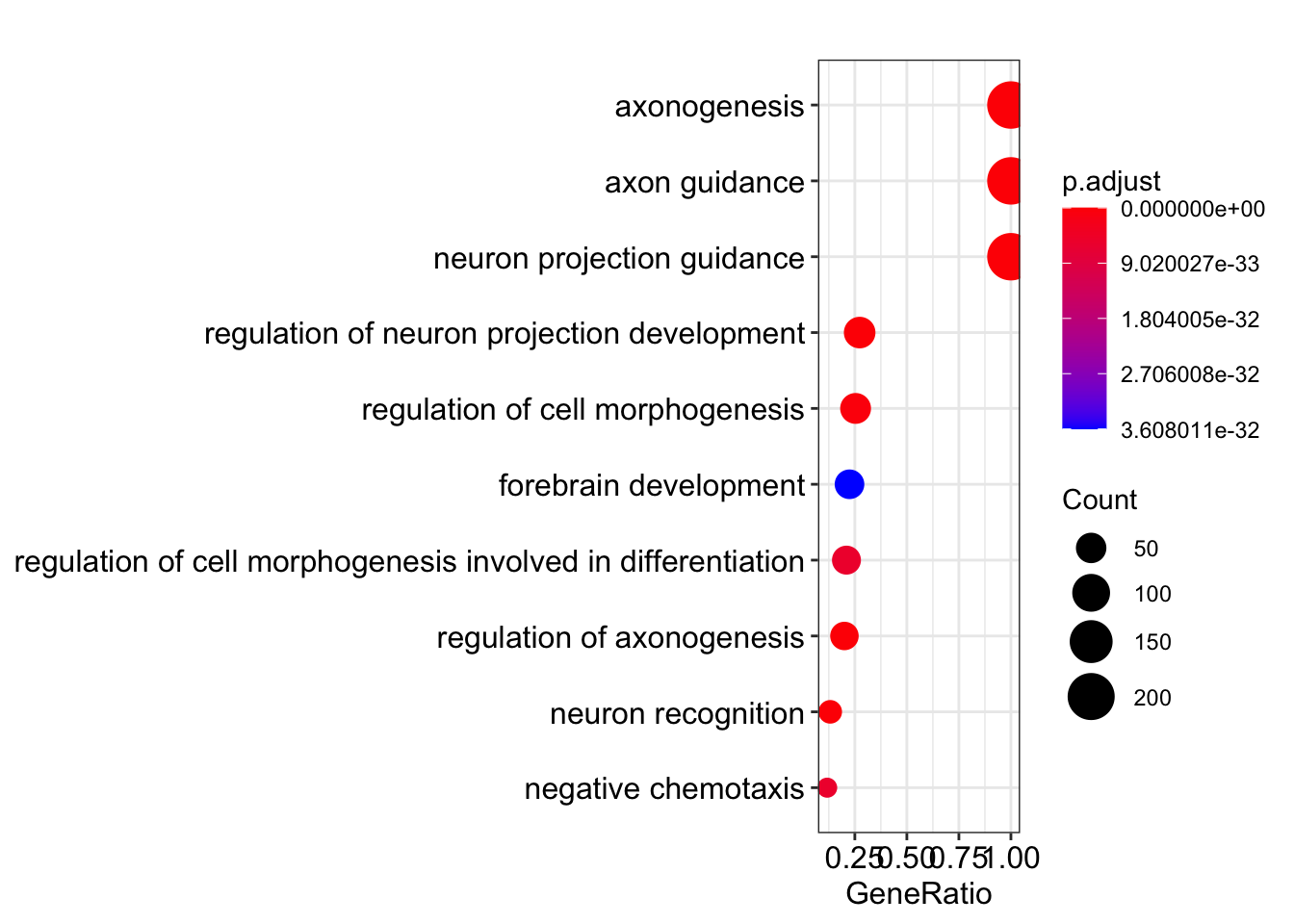
| Version | Author | Date |
|---|---|---|
| 22ec290 | davetang | 2021-01-28 |
Heat plot showing the enriched GO terms on the y-axis and the genes on the x-axis. Genes with the associated GO term are highlighted.
heatplot(my_test3, showCategory=10)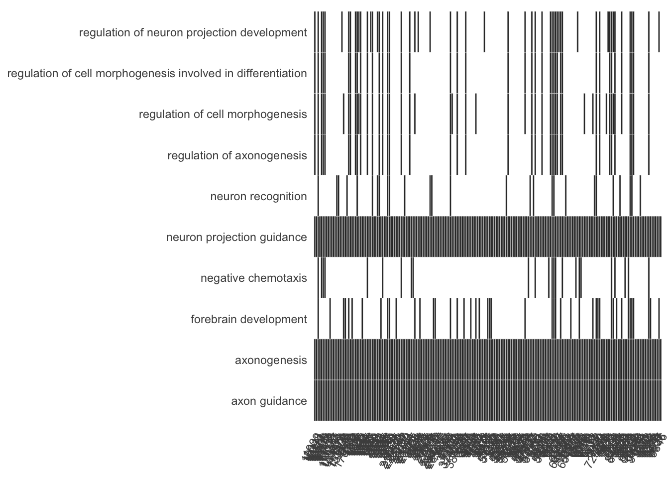
| Version | Author | Date |
|---|---|---|
| 22ec290 | davetang | 2021-01-28 |
Enrichment map organises enriched terms into a network with edges connecting overlapping gene sets.
emapplot(my_test3, showCategory = 10)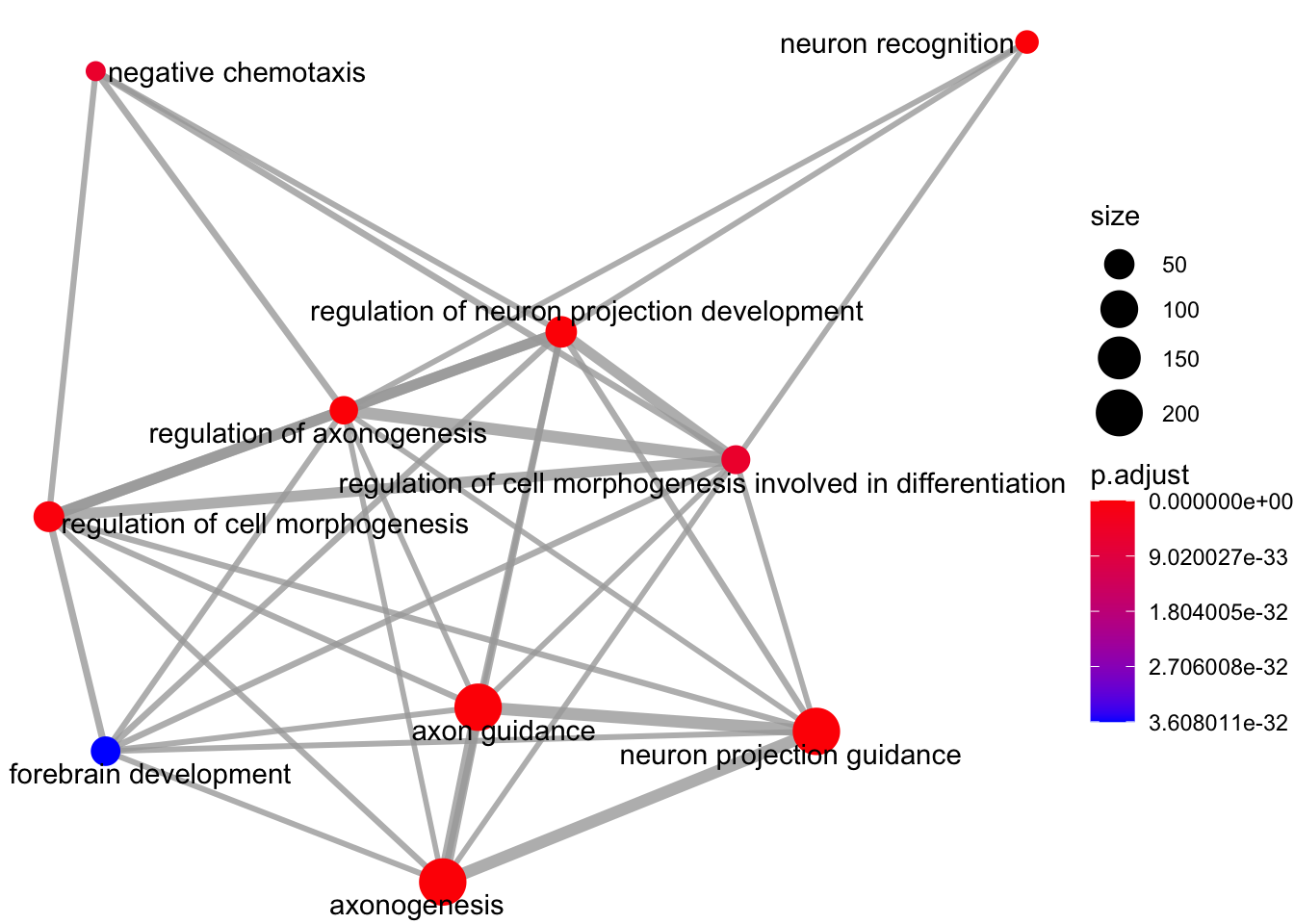
| Version | Author | Date |
|---|---|---|
| 22ec290 | davetang | 2021-01-28 |
goplot shows the gene ontology graph with the enriched GO terms highlighted.
goplot(my_test3)Warning: ggrepel: 1 unlabeled data points (too many overlaps). Consider
increasing max.overlaps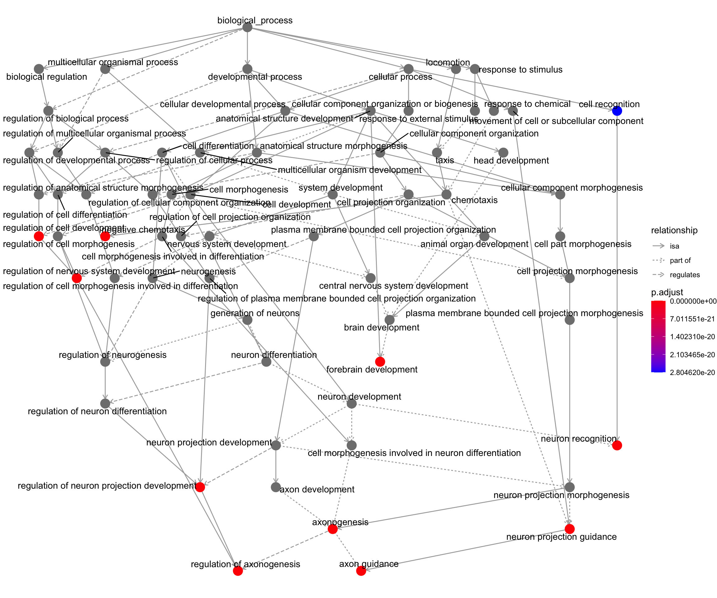
| Version | Author | Date |
|---|---|---|
| 22ec290 | davetang | 2021-01-28 |
Another nice feature of clusterProfiler is that you can plot multiple gene lists together. We can create another gene list using genes associated with GO:0010975 to demonstrate.
go_to_entrez <- select(org.Hs.eg.db,
                       keys = "GO:0010975",
                       columns = "ENTREZID",
                       keytype = "GO")
'select()' returned 1:many mapping between keys and columnsneuron_proj <- unique(go_to_entrez$ENTREZID)Perform GO enrichment on two gene lists.
my_gene_list <- list(axon = axon_gene,
                     neuron = neuron_proj)

gene_list_go <- compareCluster(geneCluster = my_gene_list,
                               fun = "enrichGO",
                               universe = universe,
                               OrgDb = org.Hs.eg.db,
                               keyType = "ENTREZID",
                               ont = "BP",
                               pvalueCutoff = 0.001,
                               pAdjustMethod = "BH",
                               qvalueCutoff = 0.1,
                               minGSSize = 10,
                               maxGSSize = 500,
                               readable = FALSE)

head(as.data.frame(gene_list_go))
Cluster ID Description GeneRatio
1 axon GO:0007409 axonogenesis 205/205
2 axon GO:0007411 axon guidance 205/205
3 axon GO:0097485 neuron projection guidance 205/205
4 axon GO:0050770 regulation of axonogenesis 41/205
5 axon GO:0008038 neuron recognition 27/205
6 axon GO:0010975 regulation of neuron projection development 56/205
BgRatio pvalue p.adjust qvalue
1 468/18670 0.000000e+00 0.000000e+00 0.000000e+00
2 276/18670 0.000000e+00 0.000000e+00 0.000000e+00
3 277/18670 0.000000e+00 0.000000e+00 0.000000e+00
4 183/18670 2.592496e-42 2.143346e-39 1.300341e-39
5 48/18670 3.898825e-41 2.578683e-38 1.564455e-38
6 499/18670 1.042084e-40 5.743620e-38 3.484583e-38
geneID
1 323/474/627/655/682/1002/1400/1436/1600/1630/1796/1808/1826/1855/1942/1943/1944/1945/1946/1947/1948/1949/1969/2041/2042/2043/2044/2045/2046/2047/2048/2049/2050/2051/2115/2131/2297/2534/2549/2625/2637/2668/2674/2675/2676/2736/2737/2817/2885/2886/2887/2909/3730/3798/3800/3897/3908/3913/4009/4089/4147/4628/4684/4756/4902/4914/4917/4983/5015/5080/5290/5291/5293/5295/5335/5458/5578/5588/5594/5595/5598/5623/5649/5747/5781/5786/5800/5818/5909/5979/6091/6092/6259/6324/6387/6405/6464/6469/6477/6585/6586/6654/6708/6709/6710/6711/6712/6714/6900/7080/7143/7204/7408/7430/7436/7473/7474/7852/7869/8013/8399/8609/8633/8660/8828/8829/8851/9046/9048/9211/9252/9260/9353/9355/9369/9378/9499/9637/9638/9846/10048/10371/10381/10500/10505/10512/10678/10752/10818/11023/11127/11313/23022/23032/23114/23191/23767/23768/26999/27020/27255/30011/51332/51466/53358/54538/55715/55740/55816/56896/57408/57453/57549/57556/57731/59277/59352/64096/64221/64855/84665/85358/89780/90249/91624/91653/128434/133418/137970/151449/152330/170302/219699/220164/223117/283297/284217/284656/285220/374946/375790/389549/644168/654429/729920
2 323/474/627/655/682/1002/1400/1436/1600/1630/1796/1808/1826/1855/1942/1943/1944/1945/1946/1947/1948/1949/1969/2041/2042/2043/2044/2045/2046/2047/2048/2049/2050/2051/2115/2131/2297/2534/2549/2625/2637/2668/2674/2675/2676/2736/2737/2817/2885/2886/2887/2909/3730/3798/3800/3897/3908/3913/4009/4089/4147/4628/4684/4756/4902/4914/4917/4983/5015/5080/5290/5291/5293/5295/5335/5458/5578/5588/5594/5595/5598/5623/5649/5747/5781/5786/5800/5818/5909/5979/6091/6092/6259/6324/6387/6405/6464/6469/6477/6585/6586/6654/6708/6709/6710/6711/6712/6714/6900/7080/7143/7204/7408/7430/7436/7473/7474/7852/7869/8013/8399/8609/8633/8660/8828/8829/8851/9046/9048/9211/9252/9260/9353/9355/9369/9378/9499/9637/9638/9846/10048/10371/10381/10500/10505/10512/10678/10752/10818/11023/11127/11313/23022/23032/23114/23191/23767/23768/26999/27020/27255/30011/51332/51466/53358/54538/55715/55740/55816/56896/57408/57453/57549/57556/57731/59277/59352/64096/64221/64855/84665/85358/89780/90249/91624/91653/128434/133418/137970/151449/152330/170302/219699/220164/223117/283297/284217/284656/285220/374946/375790/389549/644168/654429/729920
3 323/474/627/655/682/1002/1400/1436/1600/1630/1796/1808/1826/1855/1942/1943/1944/1945/1946/1947/1948/1949/1969/2041/2042/2043/2044/2045/2046/2047/2048/2049/2050/2051/2115/2131/2297/2534/2549/2625/2637/2668/2674/2675/2676/2736/2737/2817/2885/2886/2887/2909/3730/3798/3800/3897/3908/3913/4009/4089/4147/4628/4684/4756/4902/4914/4917/4983/5015/5080/5290/5291/5293/5295/5335/5458/5578/5588/5594/5595/5598/5623/5649/5747/5781/5786/5800/5818/5909/5979/6091/6092/6259/6324/6387/6405/6464/6469/6477/6585/6586/6654/6708/6709/6710/6711/6712/6714/6900/7080/7143/7204/7408/7430/7436/7473/7474/7852/7869/8013/8399/8609/8633/8660/8828/8829/8851/9046/9048/9211/9252/9260/9353/9355/9369/9378/9499/9637/9638/9846/10048/10371/10381/10500/10505/10512/10678/10752/10818/11023/11127/11313/23022/23032/23114/23191/23767/23768/26999/27020/27255/30011/51332/51466/53358/54538/55715/55740/55816/56896/57408/57453/57549/57556/57731/59277/59352/64096/64221/64855/84665/85358/89780/90249/91624/91653/128434/133418/137970/151449/152330/170302/219699/220164/223117/283297/284217/284656/285220/374946/375790/389549/644168/654429/729920
4 627/1002/1600/1630/1808/1826/1942/1946/1949/2043/2045/2048/2049/2909/3897/5458/5747/5800/5979/6091/6092/6259/6387/6405/6900/7143/7473/7474/7869/8829/8851/9353/10371/10500/10505/10512/23191/57556/89780/223117/374946
5 682/1826/1949/2042/2043/2048/2049/2909/6091/6092/6900/7852/8829/8851/10371/23022/27020/27255/54538/57453/57549/64221/84665/91624/128434/133418/152330
6 627/655/1002/1400/1600/1630/1808/1826/1855/1942/1946/1948/1949/2042/2043/2045/2048/2049/2534/2625/2909/3897/4914/5458/5649/5747/5800/5979/6091/6092/6259/6324/6387/6405/6900/7143/7436/7473/7474/7852/7869/8829/8851/9353/9638/10371/10500/10505/10512/23191/27020/57556/85358/89780/223117/374946
Count
1 205
2 205
3 205
4 41
5 27
6 56Dot plot with enriched GO terms by gene list.
dotplot(gene_list_go)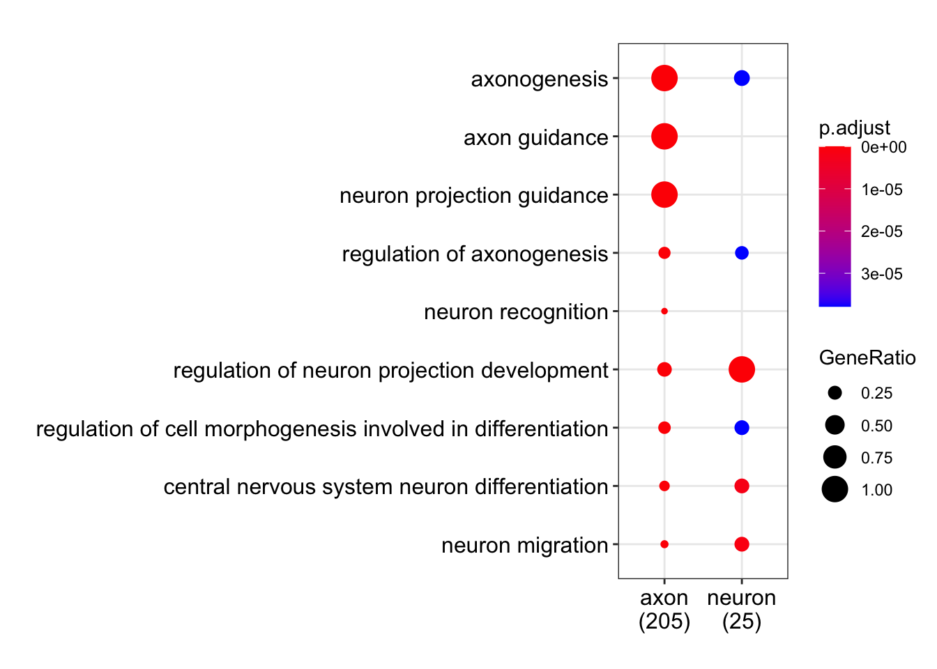
What if my gene list IDs are not Entrez gene IDs?
We can use the biomaRt package for converting between different gene identifiers and in this example, we will convert Ensembl gene IDs to Entrez gene IDs.
if (!"biomaRt" %in% installed.packages()){
  BiocManager::install("biomaRt")
}

library("biomaRt")
We will fetch every Ensembl gene ID and randomly select 10 IDs to convert into Entrez gene IDs.
ensembl <- useMart("ensembl", dataset="hsapiens_gene_ensembl")

my_chr <- c(1:22, 'M', 'X', 'Y')
my_ensembl_gene <- getBM(attributes = 'ensembl_gene_id',
                         filters = 'chromosome_name',
                         values = my_chr,
                         mart = ensembl)

head(my_ensembl_gene)
ensembl_gene_id
1 ENSG00000223972
2 ENSG00000227232
3 ENSG00000278267
4 ENSG00000243485
5 ENSG00000284332
6 ENSG00000237613Select 10 Ensembl gene IDs.
set.seed(1984)
to_convert <- sample(x = my_ensembl_gene$ensembl_gene_id, size = 10, replace = FALSE)
Now to convert the IDs.
to_entrez <- getBM(attributes = c('ensembl_gene_id', 'entrezgene_id'),
                   filters = 'ensembl_gene_id',
                   values = to_convert,
                   mart = ensembl)

to_entrez
ensembl_gene_id entrezgene_id
1 ENSG00000124568 6568
2 ENSG00000131400 9476
3 ENSG00000212191 NA
4 ENSG00000225315 NA
5 ENSG00000228658 NA
6 ENSG00000256659 101927694
7 ENSG00000257890 NA
8 ENSG00000267552 NA
9 ENSG00000280344 NA
10 ENSG00000281133 NANote that not all Ensembl IDs have Entrez IDs. We can find out how many Ensembl IDs do not have Entrez IDs.
my_entrez_gene <- getBM(attributes = c('ensembl_gene_id', 'entrezgene_id'),
                        filters = 'ensembl_gene_id',
                        values = my_ensembl_gene,
                        mart = ensembl)

table(is.na(my_entrez_gene$entrezgene_id))
FALSE  TRUE
25628 35099
35099 out of 60727 Ensembl gene IDs do not have corresponding Entrez gene IDs. To learn more about the missing Entrez ID values from the Ensembl conversion see this useful post on BioStars.
sessionInfo()R version 4.0.3 (2020-10-10)
Platform: x86_64-apple-darwin17.0 (64-bit)
Running under: macOS Big Sur 10.16
Matrix products: default
BLAS: /Library/Frameworks/R.framework/Versions/4.0/Resources/lib/libRblas.dylib
LAPACK: /Library/Frameworks/R.framework/Versions/4.0/Resources/lib/libRlapack.dylib
locale:
[1] en_AU.UTF-8/en_AU.UTF-8/en_AU.UTF-8/C/en_AU.UTF-8/en_AU.UTF-8
attached base packages:
[1] stats4 parallel stats graphics grDevices utils datasets
[8] methods base
other attached packages:
[1] biomaRt_2.44.4 org.Hs.eg.db_3.11.4 GO.db_3.11.4
[4] GOstats_2.54.0 graph_1.66.0 Category_2.54.0
[7] Matrix_1.3-2 AnnotationDbi_1.50.3 IRanges_2.22.2
[10] S4Vectors_0.26.1 Biobase_2.48.0 BiocGenerics_0.34.0
[13] clusterProfiler_3.16.1 workflowr_1.6.2
loaded via a namespace (and not attached):
[1] fgsea_1.14.0 colorspace_2.0-0 ellipsis_0.3.1
[4] ggridges_0.5.3 rprojroot_2.0.2 qvalue_2.20.0
[7] fs_1.5.0 rstudioapi_0.13 farver_2.0.3
[10] urltools_1.7.3 graphlayouts_0.7.1 ggrepel_0.9.1
[13] bit64_4.0.5 scatterpie_0.1.5 xml2_1.3.2
[16] splines_4.0.3 cachem_1.0.1 GOSemSim_2.14.2
[19] knitr_1.31 polyclip_1.10-0 jsonlite_1.7.2
[22] annotate_1.66.0 dbplyr_2.0.0 ggforce_0.3.2
[25] BiocManager_1.30.10 compiler_4.0.3 httr_1.4.2
[28] rvcheck_0.1.8 assertthat_0.2.1 fastmap_1.1.0
[31] later_1.1.0.1 tweenr_1.0.1 htmltools_0.5.1.1
[34] prettyunits_1.1.1 tools_4.0.3 igraph_1.2.6
[37] gtable_0.3.0 glue_1.4.2 reshape2_1.4.4
[40] DO.db_2.9 dplyr_1.0.3 rappdirs_0.3.2
[43] fastmatch_1.1-0 Rcpp_1.0.6 enrichplot_1.8.1
[46] vctrs_0.3.6 ggraph_2.0.4 xfun_0.20
[49] stringr_1.4.0 lifecycle_0.2.0 XML_3.99-0.5
[52] DOSE_3.14.0 europepmc_0.4 MASS_7.3-53
[55] scales_1.1.1 tidygraph_1.2.0 hms_1.0.0
[58] promises_1.1.1 RBGL_1.64.0 RColorBrewer_1.1-2
[61] curl_4.3 yaml_2.2.1 memoise_2.0.0
[64] gridExtra_2.3 ggplot2_3.3.3 downloader_0.4
[67] triebeard_0.3.0 stringi_1.5.3 RSQLite_2.2.3
[70] highr_0.8 genefilter_1.70.0 BiocParallel_1.22.0
[73] rlang_0.4.10 pkgconfig_2.0.3 bitops_1.0-6
[76] evaluate_0.14 lattice_0.20-41 purrr_0.3.4
[79] labeling_0.4.2 cowplot_1.1.1 bit_4.0.4
[82] tidyselect_1.1.0 AnnotationForge_1.30.1 GSEABase_1.50.1
[85] plyr_1.8.6 magrittr_2.0.1 R6_2.5.0
[88] generics_0.1.0 DBI_1.1.1 withr_2.4.1
[91] pillar_1.4.7 whisker_0.4 survival_3.2-7
[94] RCurl_1.98-1.2 tibble_3.0.5 crayon_1.3.4
[97] BiocFileCache_1.12.1 rmarkdown_2.6 viridis_0.5.1
[100] progress_1.2.2 grid_4.0.3 data.table_1.13.6
[103] Rgraphviz_2.32.0 blob_1.2.1 git2r_0.28.0
[106] digest_0.6.27 xtable_1.8-4 tidyr_1.1.2
[109] httpuv_1.5.5 gridGraphics_0.5-1 openssl_1.4.3
[112] munsell_0.5.0 viridisLite_0.3.0 ggplotify_0.0.5
[115] askpass_1.1