Gene expression heatmap using ARCHS4 data
2023-07-13
Last updated: 2023-07-13
Checks: 7 0
Knit directory: muse/
This reproducible R Markdown analysis was created with workflowr (version 1.7.0). The Checks tab describes the reproducibility checks that were applied when the results were created. The Past versions tab lists the development history.
Great! Since the R Markdown file has been committed to the Git repository, you know the exact version of the code that produced these results.
Great job! The global environment was empty. Objects defined in the global environment can affect the analysis in your R Markdown file in unknown ways. For reproduciblity it’s best to always run the code in an empty environment.
The command set.seed(20200712) was run prior to running
the code in the R Markdown file. Setting a seed ensures that any results
that rely on randomness, e.g. subsampling or permutations, are
reproducible.
Great job! Recording the operating system, R version, and package versions is critical for reproducibility.
Nice! There were no cached chunks for this analysis, so you can be confident that you successfully produced the results during this run.
Great job! Using relative paths to the files within your workflowr project makes it easier to run your code on other machines.
Great! You are using Git for version control. Tracking code development and connecting the code version to the results is critical for reproducibility.
The results in this page were generated with repository version 922aa56. See the Past versions tab to see a history of the changes made to the R Markdown and HTML files.
Note that you need to be careful to ensure that all relevant files for
the analysis have been committed to Git prior to generating the results
(you can use wflow_publish or
wflow_git_commit). workflowr only checks the R Markdown
file, but you know if there are other scripts or data files that it
depends on. Below is the status of the Git repository when the results
were generated:
Ignored files:
    Ignored:    .Rhistory
    Ignored:    .Rproj.user/
    Ignored:    r_packages_4.3.0/

Untracked files:
    Untracked:  analysis/cell_ranger.Rmd
    Untracked:  analysis/tss_xgboost.Rmd
    Untracked:  code/multiz100way/
    Untracked:  data/HG00702_SH089_CHSTrio.chr1.vcf.gz
    Untracked:  data/HG00702_SH089_CHSTrio.chr1.vcf.gz.tbi
    Untracked:  data/ncrna_NONCODE[v3.0].fasta.tar.gz
    Untracked:  data/ncrna_noncode_v3.fa
    Untracked:  data/netmhciipan.out.gz
    Untracked:  export/davetang039sblog.WordPress.2023-06-30.xml
    Untracked:  export/output/
    Untracked:  women.json

Unstaged changes:
    Modified:   analysis/graph.Rmd
Note that any generated files, e.g. HTML, png, CSS, etc., are not included in this status report because it is ok for generated content to have uncommitted changes.
These are the previous versions of the repository in which changes were
made to the R Markdown (analysis/gene_heatmap.Rmd) and HTML
(docs/gene_heatmap.html) files. If you’ve configured a
remote Git repository (see ?wflow_git_remote), click on the
hyperlinks in the table below to view the files as they were in that
past version.
| File | Version | Author | Date | Message |
|---|---|---|---|---|
| Rmd | 922aa56 | Dave Tang | 2023-07-13 | ARCHS4 heatmap |
Prepare data using base R.
lapply(
  list.files("data/archs4", pattern = ".csv$", full.names = TRUE),
  function(x){
    cbind(gene = sub("\\.\\w+$", "", basename(x)), read.csv(x))
  }
) |>
  do.call("rbind", args = _) -> my_df

# Split `id` column.
do.call("rbind", strsplit(x = my_df$id, split = "\\.")) |>
  as.data.frame() -> id_split

colnames(id_split) <- c('root', 'system', 'organ', 'tissue')

# Rename tissues.
cap_first <- function(x){
  s <- strsplit(x, "")[[1]][1]
  return(sub(s, toupper(s), x))
}

id_split$tissue <- tolower(id_split$tissue)
id_split$tissue <- sapply(id_split$tissue, cap_first)

my_df <- cbind(my_df, id_split)

# Order `my_df` by system.
my_df <- my_df[order(my_df$gene, my_df$system), ]
my_df$tissue <- factor(my_df$tissue, levels = unique(my_df$tissue))

head(my_df)
gene id min q1
8 ADH1C System.Cardiovascular System.Heart.VENTRICLE 1.935320 4.166910
11 ADH1C System.Cardiovascular System.Heart.ATRIUM 0.113644 2.419680
14 ADH1C System.Cardiovascular System.Heart.HEART 0.113644 0.113644
15 ADH1C System.Cardiovascular System.Heart.VALVE 0.113644 0.113644
6 ADH1C System.Connective Tissue.Adipose tissue.ADIPOSE 0.113644 4.166910
12 ADH1C System.Connective Tissue.Adipose tissue.ADIPOCYTE 0.113644 2.162720
median q3 max root system organ
8 4.93037 5.78635 7.32913 System Cardiovascular System Heart
11 4.08298 4.84279 5.79763 System Cardiovascular System Heart
14 3.17370 5.28658 7.83074 System Cardiovascular System Heart
15 3.11494 4.04248 5.81340 System Cardiovascular System Heart
6 5.53310 7.32318 8.75978 System Connective Tissue Adipose tissue
12 3.89584 6.07935 8.56720 System Connective Tissue Adipose tissue
tissue
8 Ventricle
11 Atrium
14 Heart
15 Valve
6 Adipose
12 AdipocyteBack to wide format.
my_df |>
  dplyr::select(gene, median, tissue) |>
  tidyr::pivot_wider(names_from = tissue, values_from = median) -> my_df_wide
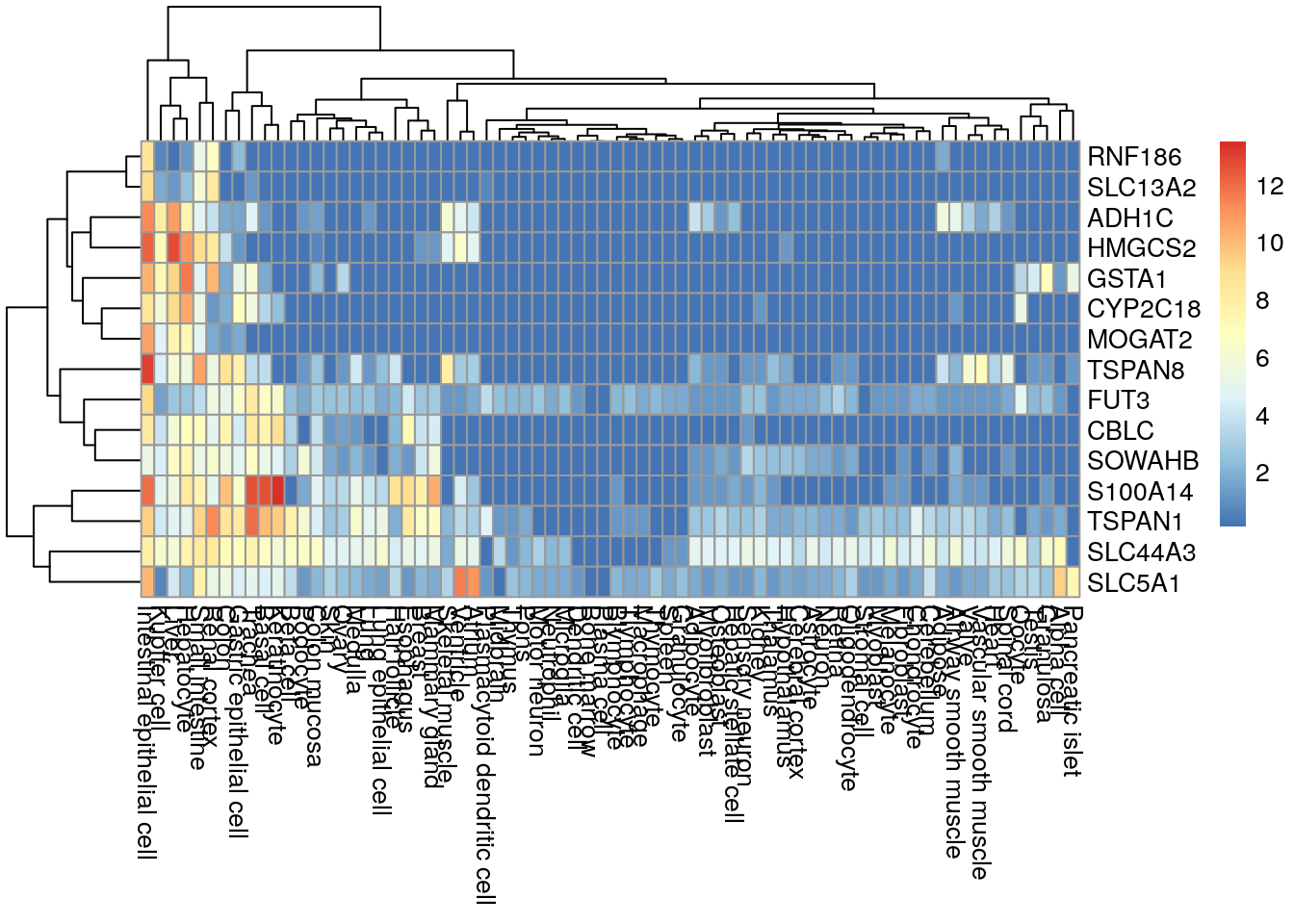
Convert to matrix and plot.
my_mat <- as.matrix(my_df_wide[, -1])
row.names(my_mat) <- my_df_wide$gene

pheatmap(my_mat)
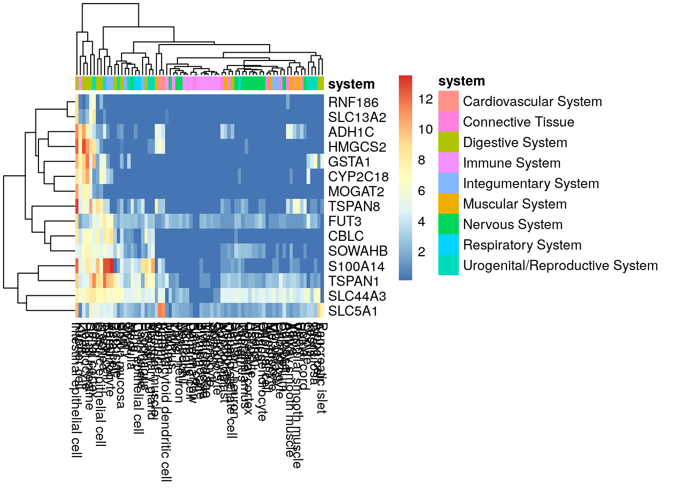
Create sample annotation.
my_order <- colnames(my_mat)

my_df |>
  dplyr::select(system, tissue) |>
  dplyr::distinct() |>
  dplyr::arrange(match(tissue, my_order)) |>
  dplyr::select(-tissue) -> sample_anno

row.names(sample_anno) <- my_order
head(sample_anno)
system
Ventricle Cardiovascular System
Atrium Cardiovascular System
Heart Cardiovascular System
Valve Cardiovascular System
Adipose Connective Tissue
Adipocyte Connective TissueHeatmap with system annotation.
pheatmap(my_mat, annotation_col = sample_anno)
sessionInfo()R version 4.3.0 (2023-04-21)
Platform: x86_64-pc-linux-gnu (64-bit)
Running under: Ubuntu 22.04.2 LTS
Matrix products: default
BLAS: /usr/lib/x86_64-linux-gnu/openblas-pthread/libblas.so.3
LAPACK: /usr/lib/x86_64-linux-gnu/openblas-pthread/libopenblasp-r0.3.20.so; LAPACK version 3.10.0
locale:
[1] LC_CTYPE=en_US.UTF-8 LC_NUMERIC=C
[3] LC_TIME=en_US.UTF-8 LC_COLLATE=en_US.UTF-8
[5] LC_MONETARY=en_US.UTF-8 LC_MESSAGES=en_US.UTF-8
[7] LC_PAPER=en_US.UTF-8 LC_NAME=C
[9] LC_ADDRESS=C LC_TELEPHONE=C
[11] LC_MEASUREMENT=en_US.UTF-8 LC_IDENTIFICATION=C
time zone: Etc/UTC
tzcode source: system (glibc)
attached base packages:
[1] stats graphics grDevices utils datasets methods base
other attached packages:
[1] pheatmap_1.0.12 workflowr_1.7.0
loaded via a namespace (and not attached):
[1] sass_0.4.5 utf8_1.2.3 generics_0.1.3 tidyr_1.3.0
[5] stringi_1.7.12 digest_0.6.31 magrittr_2.0.3 evaluate_0.20
[9] grid_4.3.0 RColorBrewer_1.1-3 fastmap_1.1.1 rprojroot_2.0.3
[13] jsonlite_1.8.5 processx_3.8.1 whisker_0.4.1 ps_1.7.5
[17] promises_1.2.0.1 httr_1.4.5 purrr_1.0.1 fansi_1.0.4
[21] scales_1.2.1 jquerylib_0.1.4 cli_3.6.1 rlang_1.1.0
[25] munsell_0.5.0 withr_2.5.0 cachem_1.0.7 yaml_2.3.7
[29] tools_4.3.0 dplyr_1.1.2 colorspace_2.1-0 httpuv_1.6.9
[33] vctrs_0.6.2 R6_2.5.1 lifecycle_1.0.3 git2r_0.32.0
[37] stringr_1.5.0 fs_1.6.2 pkgconfig_2.0.3 callr_3.7.3
[41] pillar_1.9.0 bslib_0.4.2 later_1.3.0 gtable_0.3.3
[45] glue_1.6.2 Rcpp_1.0.10 highr_0.10 xfun_0.39
[49] tibble_3.2.1 tidyselect_1.2.0 rstudioapi_0.14 knitr_1.42
[53] farver_2.1.1 htmltools_0.5.5 rmarkdown_2.21 compiler_4.3.0
[57] getPass_0.2-2