Survival analysis using the survival and survminer R packages

Last updated: 2023-11-09

Checks: 7 0

Knit directory: muse/

This reproducible R Markdown analysis was created with workflowr (version 1.7.1). The Checks tab describes the reproducibility checks that were applied when the results were created. The Past versions tab lists the development history.

R Markdown file: up-to-date

Great! Since the R Markdown file has been committed to the Git repository, you know the exact version of the code that produced these results.

Environment: empty

Great job! The global environment was empty. Objects defined in the global environment can affect the analysis in your R Markdown file in unknown ways. For reproduciblity it’s best to always run the code in an empty environment.

Seed: set.seed(20200712)

The command set.seed(20200712) was run prior to running the code in the R Markdown file. Setting a seed ensures that any results that rely on randomness, e.g. subsampling or permutations, are reproducible.

Session information: recorded

Great job! Recording the operating system, R version, and package versions is critical for reproducibility.

Cache: none

Nice! There were no cached chunks for this analysis, so you can be confident that you successfully produced the results during this run.

File paths: relative

Great job! Using relative paths to the files within your workflowr project makes it easier to run your code on other machines.

Repository version: 16f2e4c

Great! You are using Git for version control. Tracking code development and connecting the code version to the results is critical for reproducibility.

The results in this page were generated with repository version 16f2e4c. See the Past versions tab to see a history of the changes made to the R Markdown and HTML files.

Note that you need to be careful to ensure that all relevant files for the analysis have been committed to Git prior to generating the results (you can use wflow_publish or wflow_git_commit). workflowr only checks the R Markdown file, but you know if there are other scripts or data files that it depends on. Below is the status of the Git repository when the results were generated:


Ignored files:
    Ignored:    .Rhistory
    Ignored:    .Rproj.user/
    Ignored:    r_packages_4.3.2/

Untracked files:
    Untracked:  analysis/cell_ranger.Rmd
    Untracked:  analysis/sleuth.Rmd
    Untracked:  analysis/tss_xgboost.Rmd
    Untracked:  code/multiz100way/
    Untracked:  data/HG00702_SH089_CHSTrio.chr1.vcf.gz
    Untracked:  data/HG00702_SH089_CHSTrio.chr1.vcf.gz.tbi
    Untracked:  data/ncrna_NONCODE[v3.0].fasta.tar.gz
    Untracked:  data/ncrna_noncode_v3.fa
    Untracked:  data/netmhciipan.out.gz
    Untracked:  export/davetang039sblog.WordPress.2023-06-30.xml
    Untracked:  export/output/
    Untracked:  women.json

Unstaged changes:
    Modified:   analysis/graph.Rmd

Note that any generated files, e.g. HTML, png, CSS, etc., are not included in this status report because it is ok for generated content to have uncommitted changes.

These are the previous versions of the repository in which changes were made to the R Markdown (analysis/survival.Rmd) and HTML (docs/survival.html) files. If you’ve configured a remote Git repository (see ?wflow_git_remote), click on the hyperlinks in the table below to view the files as they were in that past version.

File	Version	Author	Date	Message
Rmd	16f2e4c	Dave Tang	2023-11-09	Survival analysis

Introduction

Survival analysis corresponds to a set of statistical approaches used to investigate the time it takes for an event of interest to occur. It is used in:

Cancer studies for patient’s survival time analysis
Sociology for event-history analysis
Engineering for failure-time analysis

In cancer studies, typical research questions include:

What is the impact of certain clinical characteristics on patient’s survival?
What is the probability that an individual survives 3 years?
Are there differences in survival between groups of patients?

Most survival analyses in cancer studies use the following methods:

Kaplan-Meier plots to visualise survival curves
Log-rank test to compare the survival curves of two or more groups
Cox proportional hazards regression to describe the effect of variables on survival

Basic concepts

Survival time and type of events in cancer studies

There are different types of events in cancer studies, including:

Relapse
Progression
Death

The time from “response to treatment” (complete remission) to the occurrence of the event of interest is commonly called survival time (or time to event).

The two most important measures in cancer studies include:

The time to death
The relapse-free survival time, which corresponds to the time between response to treatment and recurrence of the disease. It is also known as disease-free survival time and event-free survival time.

Censoring

Survival analysis focuses on the expected duration of time until occurrence of an event of interest (relapse or death). However, the event may not be observed for some individuals within the study time period, producing the so-called censored observations.

Censoring may arise in the following ways:

A patient has not (yet) experienced the event of interest, such as relapse or death, within the study time period;
A patient is lost to follow-up during the study period;
A patient experiences a different event that makes further follow-up impossible.

Survival and hazard functions

Two related probabilities are used to describe survival data:

The survival probability
The hazard probability

The survival probability, also known as the survivor function \(S(t)\), is the probability that an individual survives from the time origin (e.g. diagnosis of cancer) to a specified future time \(t\).

The hazard, denoted by \(h(t)\), is the probability that an individual who is under observation at a time \(t\) has an event at that time.

The survivor function focuses on not having an event and the hazard function focuses on the event occurring.

Kaplan-Meier survival estimate

The Kaplan-Meier (KM) method is a non-parametric method used to estimate the survival probability from observed survival times (Kaplan and Meier, 1958).

The survival probability at time \(t_i\), \(S(t_i)\) is calculated as follows:

\[ S(t_i) = S(t_{i-1})(1 - \frac{d_i}{n_i}) \]

Where:

\(S(t_i-1)\) = the probability of being alive at \(t_{i-1}\)
\(n_i\) = the number of patients alive just before \(t_i\)
\(d_i\) = the number of events at \(t_i\)
\(t_0 = 0\) and \(S(0) = 1\)

The estimated probability \(S(t)\) is a step function that changes value only at the time of each event. It is also possible to compute confidence intervals for the survival probability.

The KM survival curve, a plot of the KM survival probability against time, provides a useful summary of the data that can be used to estimate measures such as median survival time.

Survival analysis in R

The commonly used packages for survival analysis are

{survival} for computing survival analyses
{survminer} for summarising and visualising the results of survival analysis

Install the packages, if they are not already installed, and load them

my_packages <- c('survival', 'survminer')

sapply(my_packages, function(p){
  if(!require(p, character.only = TRUE)){
    install.packages(p)
    library(p, character.only = TRUE)
  }
  as.character(packageVersion(p))
})

 survival survminer 
  "3.5.7"   "0.4.9"

Lung cancer data

The survival package comes with lung cancer data.

data(cancer, package="survival")
str(lung)

'data.frame':   228 obs. of  10 variables:
 $ inst     : num  3 3 3 5 1 12 7 11 1 7 ...
 $ time     : num  306 455 1010 210 883 ...
 $ status   : num  2 2 1 2 2 1 2 2 2 2 ...
 $ age      : num  74 68 56 57 60 74 68 71 53 61 ...
 $ sex      : num  1 1 1 1 1 1 2 2 1 1 ...
 $ ph.ecog  : num  1 0 0 1 0 1 2 2 1 2 ...
 $ ph.karno : num  90 90 90 90 100 50 70 60 70 70 ...
 $ pat.karno: num  100 90 90 60 90 80 60 80 80 70 ...
 $ meal.cal : num  1175 1225 NA 1150 NA ...
 $ wt.loss  : num  NA 15 15 11 0 0 10 1 16 34 ...

The format of the lung data is as follows:

Column	Details
inst	Institution code
time	Survival time in days
status	censoring status 1=censored, 2=dead
age	Age in years
sex	Male=1 Female=2
ph.ecog	ECOG performance score
ph.karno	Karnofsky performance score (bad=0-good=100) rated by physician
pat.karno	Karnofsky performance score as rated by patient
meal.cal	Calories consumed at meals
wt.loss	Weight loss in last six months (pounds)

ECOG performance score is as rated by the physician.

0 = asymptomatic
1 = symptomatic but completely ambulatory
2 = in bed <50% of the day
3 = in bed > 50% of the day but not bedbound,
4 = bedbound

Compute survival curves

The function survfit() can be used to compute Kaplan-Meier survival estimates. Its main arguments include:

A survival object created using the function Surv()
The data set containing the variables

Compute the survival probability by gender.

fit <- survfit(Surv(time, status) ~ sex, data = lung)
fit

Call: survfit(formula = Surv(time, status) ~ sex, data = lung)

        n events median 0.95LCL 0.95UCL
sex=1 138    112    270     212     310
sex=2  90     53    426     348     550

Use summary(fit) to get a complete summary of the survival curves.

names(fit)

 [1] "n"         "time"      "n.risk"    "n.event"   "n.censor"  "surv"     
 [7] "std.err"   "cumhaz"    "std.chaz"  "strata"    "type"      "logse"    
[13] "conf.int"  "conf.type" "lower"     "upper"     "call"

The surv_summary() function can also be used to get a summary of survival curves.

fit_sum <- surv_summary(fit)

Warning in .get_data(x, data = data): The `data` argument is not provided. Data
will be extracted from model fit.

head(fit_sum)

  time n.risk n.event n.censor      surv    std.err     upper     lower strata
1   11    138       3        0 0.9782609 0.01268978 1.0000000 0.9542301  sex=1
2   12    135       1        0 0.9710145 0.01470747 0.9994124 0.9434235  sex=1
3   13    134       2        0 0.9565217 0.01814885 0.9911586 0.9230952  sex=1
4   15    132       1        0 0.9492754 0.01967768 0.9866017 0.9133612  sex=1
5   26    131       1        0 0.9420290 0.02111708 0.9818365 0.9038355  sex=1
6   30    130       1        0 0.9347826 0.02248469 0.9768989 0.8944820  sex=1
  sex
1   1
2   1
3   1
4   1
5   1
6   1

Name	Details
time	the time points at which the curve has a step
n.risk	the number of subjects at risk at time t
n.event	the number of events that occurred at time t
n.censor	the number of censored subjects, who exit the risk set, without an event, at time t
surv	estimate of survival probability
std.err	standard error of survival
lower,upper	lower and upper confidence limits for the curve, respectively
strata	indicates stratification of curve estimation

If strata is not NULL, there are multiple curves in the result. The levels of strata (a factor) are the labels for the curves.

Visualise survival curves

The ggsurvplot() function can be used to produce the survival curves for the two groups of subjects.

It is possible to show:

The 95% confidence limits of the survivor function using the argument conf.int = TRUE
The number and/or the percentage of individuals at risk by time using the option risk.table. Allowed values for risk.table include:
- TRUE or FALSE specifying whether to show or not the risk table. Default is FALSE
- absolute or percentage to show the absolute number and the percentage of subjects at risk by time, respectively. Use abs_pct to show both absolute number and percentage.
The p-value of the Log-Rank test comparing the groups using pval = TRUE
Horizontal/vertical line at median survival using the argument surv.median.line. Allowed values include: none, hv, h, and v

We will plot the survival plot with the following options:

Add risk table
Change risk table color by groups
Change line type by groups
Specify median survival
Use the theme_bw() ggplot2 theme
Plot the number of censored subjects at time t

ggsurvplot(
  fit,
  pval = TRUE,
  pval.method = TRUE,
  conf.int = TRUE,
  risk.table = TRUE,
  risk.table.col = "strata",
  linetype = "strata",
  surv.median.line = "hv",
  ggtheme = theme_bw(),
  ncensor.plot = TRUE,
  palette = c("#E7B800", "#2E9FDF")
)

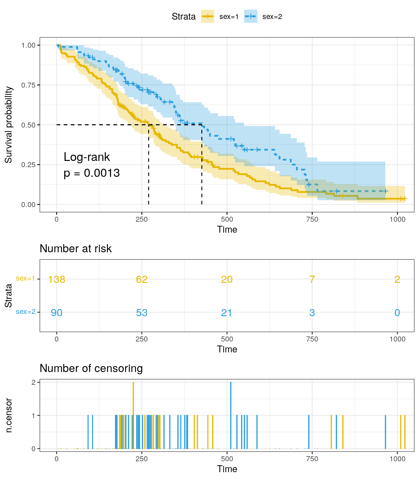
The x-axis represents time in days, and the y-axis shows the probability of surviving or the proportion of people surviving. The lines represent survival curves of the two groups. A vertical drop in the curves indicates an event, which in this case is the status (1 = censored and 2 = dead). The vertical tick mark on the curves means that a patient was censored at this time.

At time zero, the survival probability is 1.0. At time 250, the probability of survival is approximately 0.55 (or 55%) for sex=1 and 0.75 (or 75%) for sex=2. The median survival is approximately 270 days for sex=1 and 426 days for sex=2, suggesting a good survival for sex=2 compared to sex=1.

summary(fit)$table

      records n.max n.start events    rmean se(rmean) median 0.95LCL 0.95UCL
sex=1     138   138     138    112 326.0841  22.91156    270     212     310
sex=2      90    90      90     53 460.6473  34.68985    426     348     550

There appears to be a survival advantage for female with lung cancer compare to male. However, to evaluate whether this difference is statistically significant requires a formal statistical test.

Three often used transformations for ggsurvplot can be specified using the argument fun:

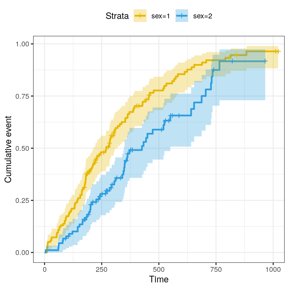
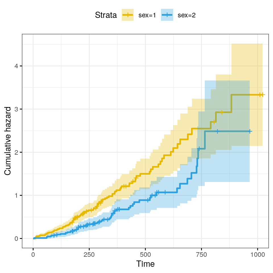
log: log transformation of the survivor function
event: plots cumulative events \(f(y) = 1-y\). It is also known as the cumulative incidence
cumhaz plots the cumulative hazard function \(f(y) = -log(y)\)

Plot cumulative events.

ggsurvplot(
  fit,
  conf.int = TRUE,
  risk.table.col = "strata",
  ggtheme = theme_bw(),
  palette = c("#E7B800", "#2E9FDF"),
  fun = "event"
)

The cumulative hazard is commonly used to estimate the hazard probability. It is defined as \(H(t) = −log(S(t))\). The cumulative hazard \(H(t)\) can be interpreted as the cumulative force of mortality. In other words, it corresponds to the number of events that would be expected for each individual by time \(t\) if the event were a repeatable process.

ggsurvplot(
  fit,
  conf.int = TRUE,
  risk.table.col = "strata",
  ggtheme = theme_bw(),
  palette = c("#E7B800", "#2E9FDF"),
  fun = "cumhaz"
)

Log-Rank test comparing survival curves

The log-rank test is the most widely used method of comparing two or more survival curves. The null hypothesis is that there is no difference in survival between the two groups. The log rank test is a non-parametric test, which makes no assumptions about the survival distributions.

Essentially, the log rank test compares the observed number of events in each group to what would be expected if the null hypothesis were true (i.e., if the survival curves were identical). The log rank statistic is approximately distributed as a chi-square test statistic.

The survdiff() function can be used to compute log-rank test comparing two or more survival curves.

sex_survdiff <- survdiff(Surv(time, status) ~ sex, data = lung)
sex_survdiff

Call:
survdiff(formula = Surv(time, status) ~ sex, data = lung)

        N Observed Expected (O-E)^2/E (O-E)^2/V
sex=1 138      112     91.6      4.55      10.3
sex=2  90       53     73.4      5.68      10.3

 Chisq= 10.3  on 1 degrees of freedom, p= 0.001

The log rank test for difference in survival gives a p-value of 0.0013112, indicating that the sex groups differ significantly in survival.

Summary

Survival analysis is a set of statistical approaches for data analysis where the outcome variable of interest is time until an event occurs.

Survival data are generally described and modeled in terms of two related functions:

The survivor function representing the probability that an individual survives from the time of origin to some time beyond time \(t\). It is usually estimated by the Kaplan-Meier method. The logrank test may be used to test for differences between survival curves for groups, such as treatments or gender as per this post.
The hazard function gives the instantaneous potential of having an event at a time, given survival up to that time. It is used primarily as a diagnostic tool or for specifying a mathematical model for survival analysis.

Take home message: The survivor function focuses on not having an event and the hazard function focuses on the event occurring.

References

Survival Analysis Basics

sessionInfo()

R version 4.3.2 (2023-10-31)
Platform: x86_64-pc-linux-gnu (64-bit)
Running under: Ubuntu 22.04.3 LTS

Matrix products: default
BLAS:   /usr/lib/x86_64-linux-gnu/openblas-pthread/libblas.so.3 
LAPACK: /usr/lib/x86_64-linux-gnu/openblas-pthread/libopenblasp-r0.3.20.so;  LAPACK version 3.10.0

locale:
 [1] LC_CTYPE=en_US.UTF-8       LC_NUMERIC=C              
 [3] LC_TIME=en_US.UTF-8        LC_COLLATE=en_US.UTF-8    
 [5] LC_MONETARY=en_US.UTF-8    LC_MESSAGES=en_US.UTF-8   
 [7] LC_PAPER=en_US.UTF-8       LC_NAME=C                 
 [9] LC_ADDRESS=C               LC_TELEPHONE=C            
[11] LC_MEASUREMENT=en_US.UTF-8 LC_IDENTIFICATION=C       

time zone: Etc/UTC
tzcode source: system (glibc)

attached base packages:
[1] stats     graphics  grDevices utils     datasets  methods   base     

other attached packages:
[1] survminer_0.4.9 ggpubr_0.6.0    ggplot2_3.4.4   survival_3.5-7 
[5] workflowr_1.7.1

loaded via a namespace (and not attached):
 [1] gtable_0.3.4      xfun_0.41         bslib_0.5.1       processx_3.8.2   
 [5] rstatix_0.7.2     lattice_0.21-9    callr_3.7.3       vctrs_0.6.4      
 [9] tools_4.3.2       ps_1.7.5          generics_0.1.3    tibble_3.2.1     
[13] fansi_1.0.5       highr_0.10        pkgconfig_2.0.3   Matrix_1.6-1.1   
[17] data.table_1.14.8 lifecycle_1.0.3   farver_2.1.1      compiler_4.3.2   
[21] stringr_1.5.0     git2r_0.32.0      munsell_0.5.0     getPass_0.2-2    
[25] carData_3.0-5     httpuv_1.6.12     htmltools_0.5.7   sass_0.4.7       
[29] yaml_2.3.7        later_1.3.1       pillar_1.9.0      car_3.1-2        
[33] jquerylib_0.1.4   whisker_0.4.1     tidyr_1.3.0       cachem_1.0.8     
[37] abind_1.4-5       km.ci_0.5-6       commonmark_1.9.0  tidyselect_1.2.0 
[41] digest_0.6.33     stringi_1.7.12    dplyr_1.1.3       purrr_1.0.2      
[45] labeling_0.4.3    splines_4.3.2     rprojroot_2.0.4   fastmap_1.1.1    
[49] grid_4.3.2        colorspace_2.1-0  cli_3.6.1         magrittr_2.0.3   
[53] utf8_1.2.4        broom_1.0.5       withr_2.5.2       scales_1.2.1     
[57] promises_1.2.1    backports_1.4.1   rmarkdown_2.25    httr_1.4.7       
[61] ggtext_0.1.2      gridExtra_2.3     ggsignif_0.6.4    zoo_1.8-12       
[65] evaluate_0.23     knitr_1.45        KMsurv_0.1-5      markdown_1.11    
[69] survMisc_0.5.6    rlang_1.1.2       gridtext_0.1.5    Rcpp_1.0.11      
[73] xtable_1.8-4      glue_1.6.2        xml2_1.3.5        rstudioapi_0.15.0
[77] jsonlite_1.8.7    R6_2.5.1          fs_1.6.3