Bartlett’s Test
2026-02-04
Last updated: 2026-02-04
Checks: 7 0
Knit directory: muse/
This reproducible R Markdown analysis was created with workflowr (version 1.7.1). The Checks tab describes the reproducibility checks that were applied when the results were created. The Past versions tab lists the development history.
Great! Since the R Markdown file has been committed to the Git repository, you know the exact version of the code that produced these results.
Great job! The global environment was empty. Objects defined in the global environment can affect the analysis in your R Markdown file in unknown ways. For reproduciblity it’s best to always run the code in an empty environment.
The command set.seed(20200712) was run prior to running
the code in the R Markdown file. Setting a seed ensures that any results
that rely on randomness, e.g. subsampling or permutations, are
reproducible.
Great job! Recording the operating system, R version, and package versions is critical for reproducibility.
Nice! There were no cached chunks for this analysis, so you can be confident that you successfully produced the results during this run.
Great job! Using relative paths to the files within your workflowr project makes it easier to run your code on other machines.
Great! You are using Git for version control. Tracking code development and connecting the code version to the results is critical for reproducibility.
The results in this page were generated with repository version 06fbf43. See the Past versions tab to see a history of the changes made to the R Markdown and HTML files.
Note that you need to be careful to ensure that all relevant files for
the analysis have been committed to Git prior to generating the results
(you can use wflow_publish or
wflow_git_commit). workflowr only checks the R Markdown
file, but you know if there are other scripts or data files that it
depends on. Below is the status of the Git repository when the results
were generated:
Ignored files:
    Ignored:    .Rproj.user/
    Ignored:    data/1M_neurons_filtered_gene_bc_matrices_h5.h5
    Ignored:    data/293t/
    Ignored:    data/293t_3t3_filtered_gene_bc_matrices.tar.gz
    Ignored:    data/293t_filtered_gene_bc_matrices.tar.gz
    Ignored:    data/5k_Human_Donor1_PBMC_3p_gem-x_5k_Human_Donor1_PBMC_3p_gem-x_count_sample_filtered_feature_bc_matrix.h5
    Ignored:    data/5k_Human_Donor2_PBMC_3p_gem-x_5k_Human_Donor2_PBMC_3p_gem-x_count_sample_filtered_feature_bc_matrix.h5
    Ignored:    data/5k_Human_Donor3_PBMC_3p_gem-x_5k_Human_Donor3_PBMC_3p_gem-x_count_sample_filtered_feature_bc_matrix.h5
    Ignored:    data/5k_Human_Donor4_PBMC_3p_gem-x_5k_Human_Donor4_PBMC_3p_gem-x_count_sample_filtered_feature_bc_matrix.h5
    Ignored:    data/97516b79-8d08-46a6-b329-5d0a25b0be98.h5ad
    Ignored:    data/Parent_SC3v3_Human_Glioblastoma_filtered_feature_bc_matrix.tar.gz
    Ignored:    data/brain_counts/
    Ignored:    data/cl.obo
    Ignored:    data/cl.owl
    Ignored:    data/jurkat/
    Ignored:    data/jurkat:293t_50:50_filtered_gene_bc_matrices.tar.gz
    Ignored:    data/jurkat_293t/
    Ignored:    data/jurkat_filtered_gene_bc_matrices.tar.gz
    Ignored:    data/pbmc20k/
    Ignored:    data/pbmc20k_seurat/
    Ignored:    data/pbmc3k.csv
    Ignored:    data/pbmc3k.csv.gz
    Ignored:    data/pbmc3k.h5ad
    Ignored:    data/pbmc3k/
    Ignored:    data/pbmc3k_bpcells_mat/
    Ignored:    data/pbmc3k_export.mtx
    Ignored:    data/pbmc3k_matrix.mtx
    Ignored:    data/pbmc3k_seurat.rds
    Ignored:    data/pbmc4k_filtered_gene_bc_matrices.tar.gz
    Ignored:    data/pbmc_1k_v3_filtered_feature_bc_matrix.h5
    Ignored:    data/pbmc_1k_v3_raw_feature_bc_matrix.h5
    Ignored:    data/refdata-gex-GRCh38-2020-A.tar.gz
    Ignored:    data/seurat_1m_neuron.rds
    Ignored:    data/t_3k_filtered_gene_bc_matrices.tar.gz
    Ignored:    r_packages_4.4.1/
    Ignored:    r_packages_4.5.0/

Untracked files:
    Untracked:  .claude/
    Untracked:  CLAUDE.md
    Untracked:  analysis/bioc.Rmd
    Untracked:  analysis/bioc_scrnaseq.Rmd
    Untracked:  analysis/chick_weight.Rmd
    Untracked:  analysis/likelihood.Rmd
    Untracked:  bpcells_matrix/
    Untracked:  data/Caenorhabditis_elegans.WBcel235.113.gtf.gz
    Untracked:  data/GCF_043380555.1-RS_2024_12_gene_ontology.gaf.gz
    Untracked:  data/SeuratObj.rds
    Untracked:  data/arab.rds
    Untracked:  data/astronomicalunit.csv
    Untracked:  data/femaleMiceWeights.csv
    Untracked:  data/lung_bcell.rds
    Untracked:  m3/
    Untracked:  women.json

Unstaged changes:
    Modified:   analysis/isoform_switch_analyzer.Rmd
    Modified:   analysis/linear_models.Rmd
Note that any generated files, e.g. HTML, png, CSS, etc., are not included in this status report because it is ok for generated content to have uncommitted changes.
These are the previous versions of the repository in which changes were
made to the R Markdown (analysis/bartlett.Rmd) and HTML
(docs/bartlett.html) files. If you’ve configured a remote
Git repository (see ?wflow_git_remote), click on the
hyperlinks in the table below to view the files as they were in that
past version.
| File | Version | Author | Date | Message |
|---|---|---|---|---|
| Rmd | 06fbf43 | Dave Tang | 2026-02-04 | Add more explanations and examples |
| html | a8aa28e | Dave Tang | 2025-12-03 | Build site. |
| Rmd | 3526ecb | Dave Tang | 2025-12-03 | Bartlett’s test |
Introduction
Bartlett’s test is used to assess whether multiple groups have equal variances, a property called homogeneity of variance (or homoscedasticity). This is an important assumption for several statistical tests, including:
- One-way ANOVA - assumes equal variances across groups
- Student’s t-test - assumes equal variances between two groups
- Linear regression - assumes constant variance of residuals
When these assumptions are violated, the test results may be unreliable.
The Hypotheses
Bartlett’s test evaluates:
- Null hypothesis (\(H_0\)): All groups have equal variances
- Alternative hypothesis (\(H_1\)): At least one group has a different variance
A small p-value (typically < 0.05) suggests rejecting the null hypothesis, indicating that variances are not equal across groups.
Important Considerations
Bartlett’s test is sensitive to departures from normality. If your data is not normally distributed, even slight deviations can cause the test to incorrectly reject the null hypothesis. Therefore:
- Use Bartlett’s test when data is approximately normal
- For non-normal data, consider the Fligner-Killeen test
(
fligner.test()), which is a non-parametric alternative available in base R.
Example 1: Unequal Variances
Let’s simulate three groups that have the same mean but different variances (standard deviations of 1, 3, and 5):
set.seed(1984)

group1 <- rnorm(50, mean = 10, sd = 1)
group2 <- rnorm(50, mean = 10, sd = 3)
group3 <- rnorm(50, mean = 10, sd = 5)

my_groups <- factor(rep(c("Group 1", "Group 2", "Group 3"), each = 50))
my_values <- c(group1, group2, group3)
eg1 <- data.frame(my_groups, my_values)
head(eg1)
my_groups my_values
1 Group 1 10.409203
2 Group 1 9.676975
3 Group 1 10.635852
4 Group 1 8.153871
5 Group 1 10.953647
6 Group 1 11.188490First, let’s examine the actual sample variances:
eg1 |>
  group_by(my_groups) |>
  summarise(
    n = n(),
    mean = round(mean(my_values), 2),
    variance = round(var(my_values), 2),
    sd = round(sd(my_values), 2)
  )
# A tibble: 3 × 5
my_groups n mean variance sd
<fct> <int> <dbl> <dbl> <dbl>
1 Group 1 50 10.2 0.91 0.95
2 Group 2 50 9.61 7.47 2.73
3 Group 3 50 9.34 24.7 4.97Now apply Bartlett’s test:
bartlett.test(my_values ~ my_groups, data = eg1)
    Bartlett test of homogeneity of variances

data:  my_values by my_groups
Bartlett's K-squared = 101, df = 2, p-value < 2.2e-16
Interpreting the Output:
- Bartlett’s K-squared: The test statistic. Larger values indicate greater differences in variances.
- df: Degrees of freedom (number of groups - 1)
- p-value: The probability of observing this test statistic if the null hypothesis were true
Here the extremely small p-value (< 0.05) leads us to reject the null hypothesis. We conclude that the variances are significantly different across groups.
Visualising the Differences
A boxplot clearly shows the different spreads:
ggplot(eg1, aes(my_groups, my_values)) +
  geom_boxplot() +
  theme_minimal() +
  labs(x = '', y = 'Values', title = 'Groups with Unequal Variances')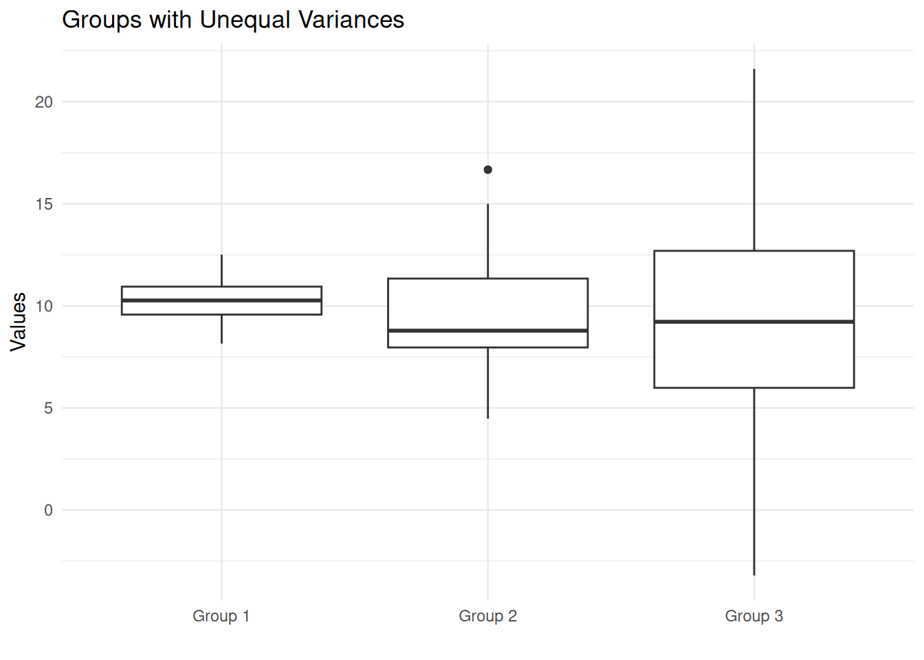
| Version | Author | Date |
|---|---|---|
| a8aa28e | Dave Tang | 2025-12-03 |
Notice how Group 1 has a narrow spread while Group 3 has a much wider spread, despite all three groups having similar centers (means around 10).
Example 2: Equal Variances
Now let’s simulate three groups with different means but similar variances (standard deviations of 2.1, 2, and 1.9):
set.seed(1984)

group1 <- rnorm(50, mean = 9,  sd = 2.1)
group2 <- rnorm(50, mean = 10, sd = 2)
group3 <- rnorm(50, mean = 11, sd = 1.9)

my_groups <- factor(rep(c("Group 1", "Group 2", "Group 3"), each = 50))
my_values <- c(group1, group2, group3)
eg2 <- data.frame(my_groups, my_values)
Check the sample variances:
eg2 |>
  group_by(my_groups) |>
  summarise(
    n = n(),
    mean = round(mean(my_values), 2),
    variance = round(var(my_values), 2),
    sd = round(sd(my_values), 2)
  )
# A tibble: 3 × 5
my_groups n mean variance sd
<fct> <int> <dbl> <dbl> <dbl>
1 Group 1 50 9.4 4.01 2
2 Group 2 50 9.74 3.32 1.82
3 Group 3 50 10.8 3.57 1.89Apply Bartlett’s test:
bartlett.test(my_values ~ my_groups, data = eg2)
    Bartlett test of homogeneity of variances

data:  my_values by my_groups
Bartlett's K-squared = 0.44385, df = 2, p-value = 0.801
The p-value is large (> 0.05), so we fail to reject the null hypothesis. There is no evidence that the variances differ across groups. This dataset would satisfy the homogeneity of variance assumption for ANOVA.
ggplot(eg2, aes(my_groups, my_values)) +
  geom_boxplot() +
  theme_minimal() +
  labs(x = '', y = 'Values', title = 'Groups with Equal Variances')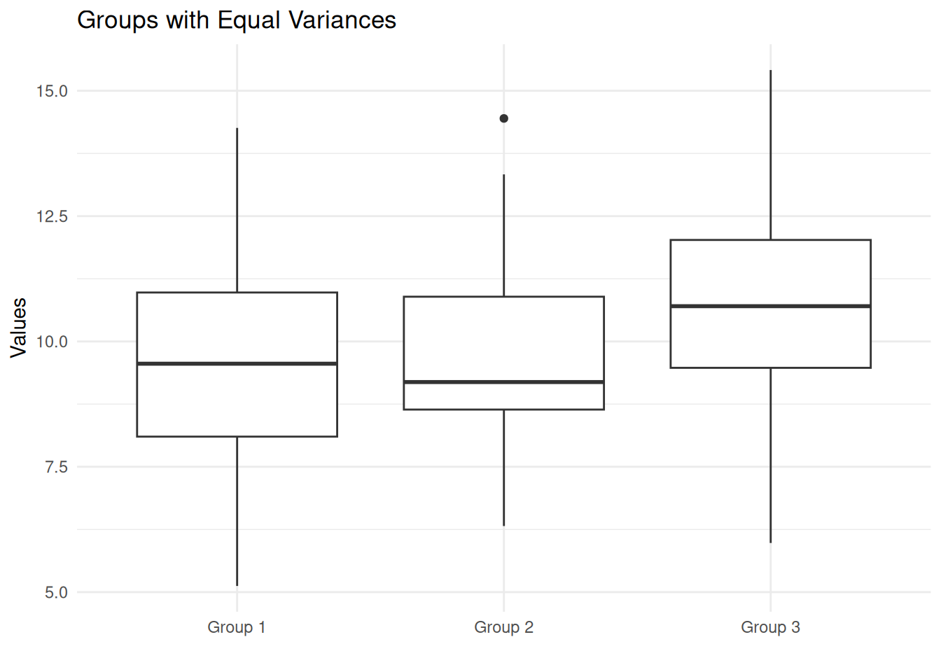
Notice the boxes have similar heights (similar interquartile ranges), reflecting the equal variances—even though the centers differ.
Real-World Example: InsectSprays Dataset
Let’s apply Bartlett’s test to the built-in InsectSprays
dataset, which contains counts of insects after treatment with different
sprays:
data(InsectSprays)
head(InsectSprays)
count spray
1 10 A
2 7 A
3 20 A
4 14 A
5 14 A
6 12 A# Examine the data
InsectSprays |>
group_by(spray) |>
summarise(
n = n(),
mean = round(mean(count), 2),
variance = round(var(count), 2)
)# A tibble: 6 × 4
spray n mean variance
<fct> <int> <dbl> <dbl>
1 A 12 14.5 22.3
2 B 12 15.3 18.2
3 C 12 2.08 3.9
4 D 12 4.92 6.27
5 E 12 3.5 3
6 F 12 16.7 38.6 bartlett.test(count ~ spray, data = InsectSprays)
    Bartlett test of homogeneity of variances

data:  count by spray
Bartlett's K-squared = 25.96, df = 5, p-value = 9.085e-05
The very small p-value indicates that variances are significantly different across spray types. Before running ANOVA on this data, we would need to address this violation (e.g., transform the data or use Welch’s ANOVA).
ggplot(InsectSprays, aes(spray, count)) +
  geom_boxplot() +
  theme_minimal() +
  labs(x = 'Spray Type', y = 'Insect Count', title = 'InsectSprays Dataset')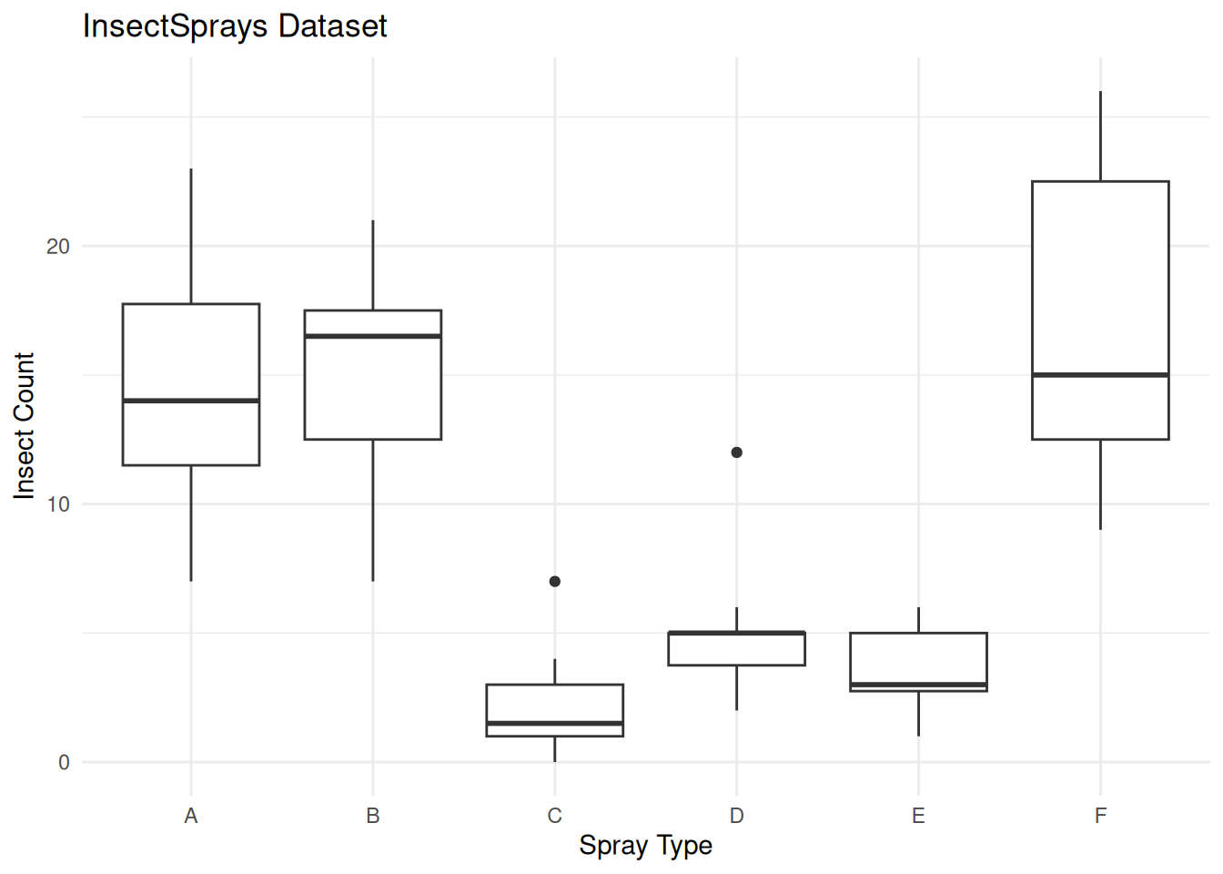
Alternative: Fligner-Killeen Test
When data is not normally distributed, the Fligner-Killeen test is a robust alternative. It is a non-parametric test based on ranks, making it resistant to departures from normality:
fligner.test(my_values ~ my_groups, data = eg1)
    Fligner-Killeen test of homogeneity of variances

data:  my_values by my_groups
Fligner-Killeen:med chi-squared = 40.611, df = 2, p-value = 1.519e-09
Like Bartlett’s test, a small p-value indicates unequal variances. The Fligner-Killeen test also rejects the null hypothesis here, confirming that variances differ across groups.
Let’s also check the equal variance example:
fligner.test(my_values ~ my_groups, data = eg2)
    Fligner-Killeen test of homogeneity of variances

data:  my_values by my_groups
Fligner-Killeen:med chi-squared = 0.7194, df = 2, p-value = 0.6979
As expected, the test does not reject the null hypothesis for the equal variance data.
Summary
| Test | When to Use | R Function |
|---|---|---|
| Bartlett’s test | Data is normally distributed | bartlett.test() |
| Fligner-Killeen test | Non-parametric alternative | fligner.test() |
Key points:
- Bartlett’s test checks if group variances are equal (homoscedasticity)
- It is sensitive to non-normality—use Fligner-Killeen for non-normal data
- A significant result (p < 0.05) means variances are unequal
- Unequal variances may require data transformation or using robust methods (e.g., Welch’s ANOVA)
sessionInfo()R version 4.5.0 (2025-04-11)
Platform: x86_64-pc-linux-gnu
Running under: Ubuntu 24.04.3 LTS
Matrix products: default
BLAS: /usr/lib/x86_64-linux-gnu/openblas-pthread/libblas.so.3
LAPACK: /usr/lib/x86_64-linux-gnu/openblas-pthread/libopenblasp-r0.3.26.so; LAPACK version 3.12.0
locale:
[1] LC_CTYPE=en_US.UTF-8 LC_NUMERIC=C
[3] LC_TIME=en_US.UTF-8 LC_COLLATE=en_US.UTF-8
[5] LC_MONETARY=en_US.UTF-8 LC_MESSAGES=en_US.UTF-8
[7] LC_PAPER=en_US.UTF-8 LC_NAME=C
[9] LC_ADDRESS=C LC_TELEPHONE=C
[11] LC_MEASUREMENT=en_US.UTF-8 LC_IDENTIFICATION=C
time zone: Etc/UTC
tzcode source: system (glibc)
attached base packages:
[1] stats graphics grDevices utils datasets methods base
other attached packages:
[1] lubridate_1.9.4 forcats_1.0.0 stringr_1.5.1 dplyr_1.1.4
[5] purrr_1.0.4 readr_2.1.5 tidyr_1.3.1 tibble_3.3.0
[9] ggplot2_3.5.2 tidyverse_2.0.0 workflowr_1.7.1
loaded via a namespace (and not attached):
[1] utf8_1.2.6 sass_0.4.10 generics_0.1.4 stringi_1.8.7
[5] hms_1.1.3 digest_0.6.37 magrittr_2.0.3 timechange_0.3.0
[9] evaluate_1.0.3 grid_4.5.0 RColorBrewer_1.1-3 fastmap_1.2.0
[13] rprojroot_2.0.4 jsonlite_2.0.0 processx_3.8.6 whisker_0.4.1
[17] ps_1.9.1 promises_1.3.3 httr_1.4.7 scales_1.4.0
[21] jquerylib_0.1.4 cli_3.6.5 rlang_1.1.6 withr_3.0.2
[25] cachem_1.1.0 yaml_2.3.10 tools_4.5.0 tzdb_0.5.0
[29] httpuv_1.6.16 vctrs_0.6.5 R6_2.6.1 lifecycle_1.0.4
[33] git2r_0.36.2 fs_1.6.6 pkgconfig_2.0.3 callr_3.7.6
[37] pillar_1.10.2 bslib_0.9.0 later_1.4.2 gtable_0.3.6
[41] glue_1.8.0 Rcpp_1.0.14 xfun_0.52 tidyselect_1.2.1
[45] rstudioapi_0.17.1 knitr_1.50 farver_2.1.2 htmltools_0.5.8.1
[49] labeling_0.4.3 rmarkdown_2.29 compiler_4.5.0 getPass_0.2-4