Chi-squared Tests
2026-02-04
Last updated: 2026-02-04
Checks: 7 0
Knit directory: muse/
This reproducible R Markdown analysis was created with workflowr (version 1.7.1). The Checks tab describes the reproducibility checks that were applied when the results were created. The Past versions tab lists the development history.
Great! Since the R Markdown file has been committed to the Git repository, you know the exact version of the code that produced these results.
Great job! The global environment was empty. Objects defined in the global environment can affect the analysis in your R Markdown file in unknown ways. For reproduciblity it’s best to always run the code in an empty environment.
The command set.seed(20200712) was run prior to running
the code in the R Markdown file. Setting a seed ensures that any results
that rely on randomness, e.g. subsampling or permutations, are
reproducible.
Great job! Recording the operating system, R version, and package versions is critical for reproducibility.
Nice! There were no cached chunks for this analysis, so you can be confident that you successfully produced the results during this run.
Great job! Using relative paths to the files within your workflowr project makes it easier to run your code on other machines.
Great! You are using Git for version control. Tracking code development and connecting the code version to the results is critical for reproducibility.
The results in this page were generated with repository version 393faf7. See the Past versions tab to see a history of the changes made to the R Markdown and HTML files.
Note that you need to be careful to ensure that all relevant files for
the analysis have been committed to Git prior to generating the results
(you can use wflow_publish or
wflow_git_commit). workflowr only checks the R Markdown
file, but you know if there are other scripts or data files that it
depends on. Below is the status of the Git repository when the results
were generated:
Ignored files:
    Ignored:    .Rproj.user/
    Ignored:    data/1M_neurons_filtered_gene_bc_matrices_h5.h5
    Ignored:    data/293t/
    Ignored:    data/293t_3t3_filtered_gene_bc_matrices.tar.gz
    Ignored:    data/293t_filtered_gene_bc_matrices.tar.gz
    Ignored:    data/5k_Human_Donor1_PBMC_3p_gem-x_5k_Human_Donor1_PBMC_3p_gem-x_count_sample_filtered_feature_bc_matrix.h5
    Ignored:    data/5k_Human_Donor2_PBMC_3p_gem-x_5k_Human_Donor2_PBMC_3p_gem-x_count_sample_filtered_feature_bc_matrix.h5
    Ignored:    data/5k_Human_Donor3_PBMC_3p_gem-x_5k_Human_Donor3_PBMC_3p_gem-x_count_sample_filtered_feature_bc_matrix.h5
    Ignored:    data/5k_Human_Donor4_PBMC_3p_gem-x_5k_Human_Donor4_PBMC_3p_gem-x_count_sample_filtered_feature_bc_matrix.h5
    Ignored:    data/97516b79-8d08-46a6-b329-5d0a25b0be98.h5ad
    Ignored:    data/Parent_SC3v3_Human_Glioblastoma_filtered_feature_bc_matrix.tar.gz
    Ignored:    data/brain_counts/
    Ignored:    data/cl.obo
    Ignored:    data/cl.owl
    Ignored:    data/jurkat/
    Ignored:    data/jurkat:293t_50:50_filtered_gene_bc_matrices.tar.gz
    Ignored:    data/jurkat_293t/
    Ignored:    data/jurkat_filtered_gene_bc_matrices.tar.gz
    Ignored:    data/pbmc20k/
    Ignored:    data/pbmc20k_seurat/
    Ignored:    data/pbmc3k.csv
    Ignored:    data/pbmc3k.csv.gz
    Ignored:    data/pbmc3k.h5ad
    Ignored:    data/pbmc3k/
    Ignored:    data/pbmc3k_bpcells_mat/
    Ignored:    data/pbmc3k_export.mtx
    Ignored:    data/pbmc3k_matrix.mtx
    Ignored:    data/pbmc3k_seurat.rds
    Ignored:    data/pbmc4k_filtered_gene_bc_matrices.tar.gz
    Ignored:    data/pbmc_1k_v3_filtered_feature_bc_matrix.h5
    Ignored:    data/pbmc_1k_v3_raw_feature_bc_matrix.h5
    Ignored:    data/refdata-gex-GRCh38-2020-A.tar.gz
    Ignored:    data/seurat_1m_neuron.rds
    Ignored:    data/t_3k_filtered_gene_bc_matrices.tar.gz
    Ignored:    r_packages_4.4.1/
    Ignored:    r_packages_4.5.0/

Untracked files:
    Untracked:  .claude/
    Untracked:  CLAUDE.md
    Untracked:  analysis/bioc.Rmd
    Untracked:  analysis/bioc_scrnaseq.Rmd
    Untracked:  analysis/chick_weight.Rmd
    Untracked:  analysis/likelihood.Rmd
    Untracked:  bpcells_matrix/
    Untracked:  data/Caenorhabditis_elegans.WBcel235.113.gtf.gz
    Untracked:  data/GCF_043380555.1-RS_2024_12_gene_ontology.gaf.gz
    Untracked:  data/SeuratObj.rds
    Untracked:  data/arab.rds
    Untracked:  data/astronomicalunit.csv
    Untracked:  data/femaleMiceWeights.csv
    Untracked:  data/lung_bcell.rds
    Untracked:  m3/
    Untracked:  women.json

Unstaged changes:
    Modified:   analysis/isoform_switch_analyzer.Rmd
    Modified:   analysis/linear_models.Rmd
Note that any generated files, e.g. HTML, png, CSS, etc., are not included in this status report because it is ok for generated content to have uncommitted changes.
These are the previous versions of the repository in which changes were
made to the R Markdown (analysis/chi.Rmd) and HTML
(docs/chi.html) files. If you’ve configured a remote Git
repository (see ?wflow_git_remote), click on the hyperlinks
in the table below to view the files as they were in that past version.
| File | Version | Author | Date | Message |
|---|---|---|---|---|
| Rmd | 393faf7 | Dave Tang | 2026-02-04 | Update |
| html | 503ceec | Dave Tang | 2025-11-14 | Build site. |
| Rmd | dddb710 | Dave Tang | 2025-11-14 | Chi-squared tests |
Introduction
The chi-squared (\(\chi^2\)) test is one of the most widely used statistical tests for categorical data. There are two main types:
- Chi-squared test of independence: Tests whether two categorical variables are related
- Chi-squared goodness of fit test: Tests whether observed frequencies match expected frequencies
Common applications include:
- Is smoking related to lung cancer?
- Is gender related to voting preference?
- Does a die produce fair outcomes?
- Is a treatment associated with recovery?
The Chi-Squared Distribution
The chi-squared distribution arises when summing squared standard normal random variables. It has one parameter: degrees of freedom (df), which determines its shape.
x <- seq(0, 20, length = 200)

plot(x, dchisq(x, df = 1), type = "l", lwd = 2, col = 1,
     ylim = c(0, 0.5), ylab = "Density", xlab = "Chi-squared value",
     main = "Chi-squared distributions")
lines(x, dchisq(x, df = 2), lwd = 2, col = 2)
lines(x, dchisq(x, df = 5), lwd = 2, col = 3)
lines(x, dchisq(x, df = 10), lwd = 2, col = 4)
legend("topright", legend = paste("df =", c(1, 2, 5, 10)),
       col = 1:4, lwd = 2)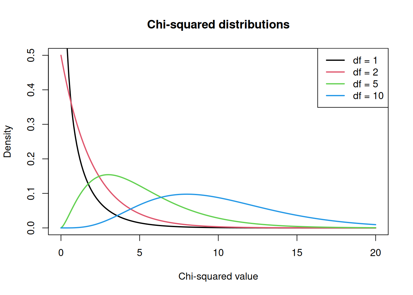
As degrees of freedom increase, the distribution becomes more symmetric and shifts to the right.
Chi-Squared Test of Independence
This test determines whether there is a statistically significant association between two categorical variables.
Hypotheses
- Null hypothesis (\(H_0\)): The two variables are independent (no association)
- Alternative hypothesis (\(H_1\)): The two variables are not independent (there is an association)
The Test Statistic
The chi-squared statistic measures the discrepancy between observed and expected frequencies:
\[\chi^2 = \sum \frac{(O - E)^2}{E}\]
where:
- \(O\) = observed frequency in each cell
- \(E\) = expected frequency if variables were independent
The expected frequency for each cell is calculated as:
\[E = \frac{\text{row total} \times \text{column total}}{\text{grand total}}\]
Example 1: Smoking and Lung Cancer
Let’s test whether smoking is associated with lung cancer using a 2x2 contingency table.
data <- matrix(
  c(60, 40, 30, 70),
  nrow = 2,
  byrow = TRUE
)

colnames(data) <- c("Cancer", "NoCancer")
rownames(data) <- c("Smoker", "NonSmoker")

data
Cancer NoCancer
Smoker 60 40
NonSmoker 30 70Step 1: Calculate Expected Values
If smoking and cancer were independent, we would expect each cell to have:
\[E = \frac{\text{row total} \times \text{column total}}{\text{grand total}}\]
# Row and column totals
row_totals <- rowSums(data)
col_totals <- colSums(data)
grand_total <- sum(data)

row_totals
Smoker NonSmoker
100 100 col_totals Cancer NoCancer
90 110 grand_total[1] 200# Calculate expected values
expected <- outer(row_totals, col_totals) / grand_total
expected Cancer NoCancer
Smoker 45 55
NonSmoker 45 55For example, the expected count for Smoker + Cancer is: \((100 \times 90) / 200 = 45\)
Step 2: Calculate the Chi-Squared Statistic
# Chi-squared = sum of (observed - expected)^2 / expected
chi_sq <- sum((data - expected)^2 / expected)
chi_sq
[1] 18.18182Step 3: Run the Test
result <- chisq.test(data)
result
    Pearson's Chi-squared test with Yates' continuity correction

data:  data
X-squared = 16.99, df = 1, p-value = 3.758e-05
Interpreting the Output
- X-squared = 16.99: The test statistic measuring how different observed values are from expected values
- df = 1: Degrees of freedom = (rows - 1) x (columns - 1) = 1 for a 2x2 table
- p-value = 3.76e-05: Probability of seeing this extreme a result if the null hypothesis were true
Since the p-value is very small (< 0.05), we reject the null hypothesis and conclude that smoking and lung cancer are associated.
Accessing Test Components
The test object contains useful information:
# Observed values
result$observed
Cancer NoCancer
Smoker 60 40
NonSmoker 30 70# Expected values (same as our manual calculation)
result$expected Cancer NoCancer
Smoker 45 55
NonSmoker 45 55# Residuals: (observed - expected) / sqrt(expected)
result$residuals Cancer NoCancer
Smoker 2.236068 -2.0226
NonSmoker -2.236068 2.0226Residuals show which cells contribute most to the chi-squared statistic. Large positive residuals indicate more observations than expected; large negative residuals indicate fewer.
Visualising the Result
x2 <- result$statistic
df <- result$parameter

x <- seq(0, x2 + 3, length = 500)

plot(x, dchisq(x, df), type = "l", lwd = 2,
     ylab = "Density", xlab = "Chi-squared value",
     main = paste0("Chi-squared distribution (df = ", df, ")"))
abline(v = x2, col = "red", lwd = 2)

# Shade the rejection region
x_shade <- seq(x2, x2 + 3, length = 100)
polygon(c(x_shade, rev(x_shade)),
        c(dchisq(x_shade, df), rep(0, length(x_shade))),
        col = rgb(1, 0, 0, 0.3), border = NA)
text(x2, 0.1, paste("p =", format.pval(result$p.value, digits = 2)),
     pos = 4, col = "red")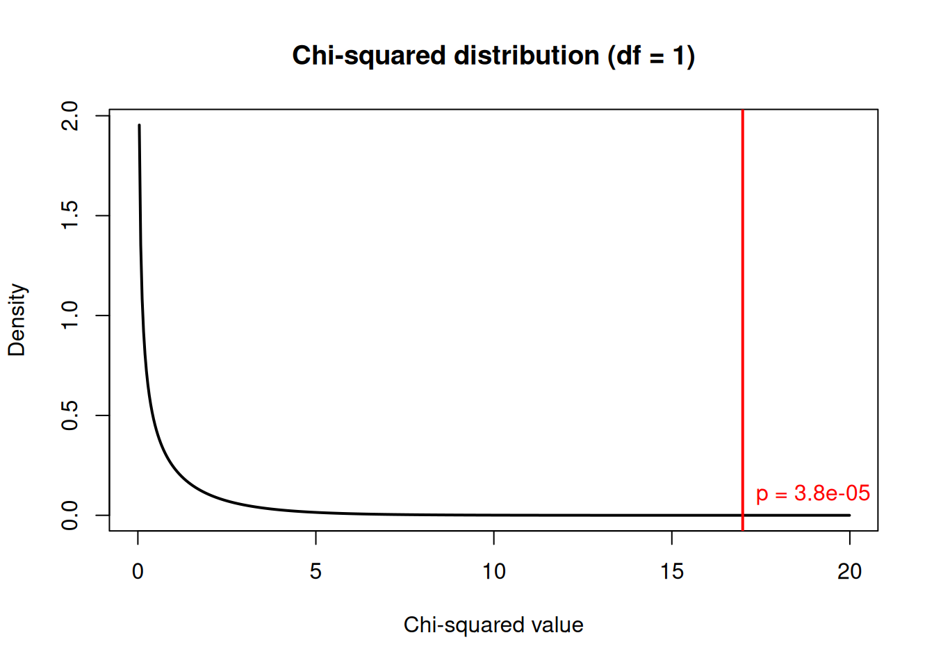
| Version | Author | Date |
|---|---|---|
| 503ceec | Dave Tang | 2025-11-14 |
The red line shows our test statistic. The shaded area represents the p-value: the probability of getting a value this extreme or more extreme under the null hypothesis.
Example 2: Larger Contingency Table
Chi-squared tests work for tables larger than 2x2. Let’s examine the relationship between education level and job satisfaction:
# Create a 3x3 table
job_data <- matrix(
  c(20, 25, 15,    # High school
    30, 40, 20,    # Bachelor's
    15, 30, 25),   # Graduate
  nrow = 3,
  byrow = TRUE
)

colnames(job_data) <- c("Low", "Medium", "High")
rownames(job_data) <- c("HighSchool", "Bachelors", "Graduate")

job_data
Low Medium High
HighSchool 20 25 15
Bachelors 30 40 20
Graduate 15 30 25result2 <- chisq.test(job_data)
result2
    Pearson's Chi-squared test

data:  job_data
X-squared = 5.1406, df = 4, p-value = 0.2732
For a 3x3 table, df = (3-1) x (3-1) = 4.
# View expected values
round(result2$expected, 1)
Low Medium High
HighSchool 17.7 25.9 16.4
Bachelors 26.6 38.9 24.5
Graduate 20.7 30.2 19.1The p-value of 0.273 suggests a marginally significant association between education and job satisfaction.
Example 3: No Association
To understand what “no association” looks like, let’s create data where the variables are independent:
set.seed(1984)

# Generate independent data
n <- 200
gender <- sample(c("Male", "Female"), n, replace = TRUE)
preference <- sample(c("Tea", "Coffee"), n, replace = TRUE)

indep_table <- table(gender, preference)
indep_table
preference
gender Coffee Tea
Female 53 50
Male 51 46chisq.test(indep_table)
    Pearson's Chi-squared test with Yates' continuity correction

data:  indep_table
X-squared = 0.00028872, df = 1, p-value = 0.9864
With a large p-value, we fail to reject the null hypothesis. There is no evidence of an association between gender and beverage preference in this simulated data.
Chi-Squared Goodness of Fit Test
This test compares observed frequencies to expected frequencies based on a theoretical distribution.
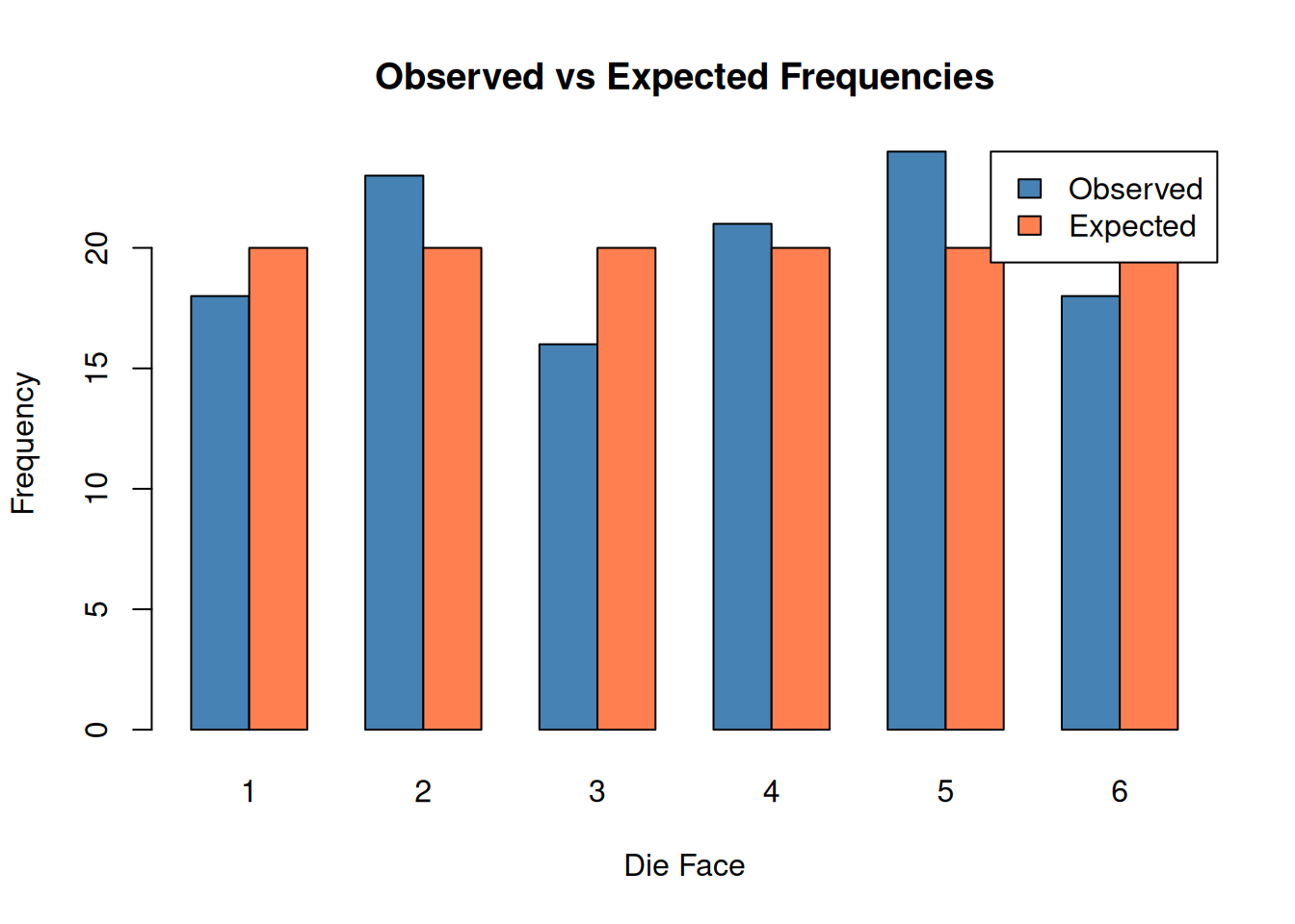
Example: Is a Die Fair?
Suppose we roll a die 120 times and observe the following counts:
observed <- c(18, 23, 16, 21, 24, 18)
names(observed) <- 1:6

# Expected: equal probability for each face
expected_prob <- rep(1/6, 6)

# Goodness of fit test
gof_result <- chisq.test(observed, p = expected_prob)
gof_result
    Chi-squared test for given probabilities

data:  observed
X-squared = 2.5, df = 5, p-value = 0.7765
The large p-value suggests we cannot reject the hypothesis that the die is fair.
barplot(
  rbind(observed, expected_prob * sum(observed)),
  beside = TRUE,
  col = c("steelblue", "coral"),
  names.arg = 1:6,
  xlab = "Die Face",
  ylab = "Frequency",
  main = "Observed vs Expected Frequencies",
  legend.text = c("Observed", "Expected"),
  args.legend = list(x = "topright")
)
Example: Testing a Genetic Ratio
In genetics, Mendel’s law predicts a 9:3:3:1 ratio for certain crosses. Let’s test whether observed data follows this ratio:
observed_plants <- c(315, 108, 101, 32)
names(observed_plants) <- c("Round-Yellow", "Round-Green",
                            "Wrinkled-Yellow", "Wrinkled-Green")

# Expected ratio 9:3:3:1
expected_ratio <- c(9, 3, 3, 1) / 16

mendel_test <- chisq.test(observed_plants, p = expected_ratio)
mendel_test
    Chi-squared test for given probabilities

data:  observed_plants
X-squared = 0.47002, df = 3, p-value = 0.9254
The p-value of 0.925 indicates the observed data is consistent with the expected 9:3:3:1 ratio.
Assumptions and Conditions
The chi-squared test has several assumptions:
- Independence: Observations must be independent
- Random sampling: Data should come from a random sample
- Expected frequencies: All expected cell counts should be at least 5
Checking Expected Frequencies
# Check expected values
result$expected
Cancer NoCancer
Smoker 45 55
NonSmoker 45 55# All expected values >= 5, so assumption is met
all(result$expected >= 5)[1] TRUEWhen Assumptions Are Violated
If expected frequencies are too small (< 5), consider:
- Fisher’s exact test: For 2x2 tables with small samples
- Combining categories: Merge cells to increase expected counts
- Simulation-based p-value: Use
chisq.test(..., simulate.p.value = TRUE)
# Small sample example
small_data <- matrix(c(3, 2, 1, 4), nrow = 2)
rownames(small_data) <- c("Treatment", "Control")
colnames(small_data) <- c("Success", "Failure")

small_data
Success Failure
Treatment 3 1
Control 2 4# Chi-squared test warns about small expected values
chisq.test(small_data)Warning in chisq.test(small_data): Chi-squared approximation may be incorrect
    Pearson's Chi-squared test with Yates' continuity correction

data:  small_data
X-squared = 0.41667, df = 1, p-value = 0.5186
# Use Fisher's exact test instead
fisher.test(small_data)
    Fisher's Exact Test for Count Data

data:  small_data
p-value = 0.5238
alternative hypothesis: true odds ratio is not equal to 1
95 percent confidence interval:
   0.218046 390.562917
sample estimates:
odds ratio
  4.918388
Effect Size: Cramer’s V
A significant p-value tells us an association exists, but not how strong it is. Cramer’s V measures effect size for chi-squared tests:
\[V = \sqrt{\frac{\chi^2}{n \times (k - 1)}}\]
where \(n\) is the sample size and \(k\) is the smaller of the number of rows or columns.
# Calculate Cramer's V for the smoking example
chi_sq <- result$statistic
n <- sum(data)
k <- min(nrow(data), ncol(data))

cramers_v <- sqrt(chi_sq / (n * (k - 1)))
cramers_v
X-squared
0.291461 Interpretation guidelines for Cramer’s V:
| V | Interpretation |
|---|---|
| 0.1 | Small effect |
| 0.3 | Medium effect |
| 0.5 | Large effect |
A Cramer’s V of 0.29 indicates a small to medium effect size. # Yates’ Continuity Correction
For 2x2 tables, R applies Yates’ continuity correction by default. This makes the test more conservative (larger p-values) but can be overly conservative with moderate sample sizes.
# With Yates' correction (default)
chisq.test(data)
    Pearson's Chi-squared test with Yates' continuity correction

data:  data
X-squared = 16.99, df = 1, p-value = 3.758e-05
# Without Yates' correction
chisq.test(data, correct = FALSE)
    Pearson's Chi-squared test

data:  data
X-squared = 18.182, df = 1, p-value = 2.008e-05
The uncorrected version gives a slightly smaller p-value. For large samples, the difference is negligible.
Summary
| Test | Purpose | R Function |
|---|---|---|
| Test of independence | Association between two categorical variables | chisq.test(table) |
| Goodness of fit | Compare observed to expected frequencies | chisq.test(x, p = prob) |
| Fisher’s exact test | Small samples (expected < 5) | fisher.test(table) |
Key points:
- Chi-squared tests assess relationships between categorical variables
- The test statistic measures how much observed differs from expected
- Larger chi-squared values indicate stronger evidence against independence
- Check that expected frequencies are at least 5
- Use Cramer’s V to measure effect size
- For small samples, use Fisher’s exact test instead
sessionInfo()R version 4.5.0 (2025-04-11)
Platform: x86_64-pc-linux-gnu
Running under: Ubuntu 24.04.3 LTS
Matrix products: default
BLAS: /usr/lib/x86_64-linux-gnu/openblas-pthread/libblas.so.3
LAPACK: /usr/lib/x86_64-linux-gnu/openblas-pthread/libopenblasp-r0.3.26.so; LAPACK version 3.12.0
locale:
[1] LC_CTYPE=en_US.UTF-8 LC_NUMERIC=C
[3] LC_TIME=en_US.UTF-8 LC_COLLATE=en_US.UTF-8
[5] LC_MONETARY=en_US.UTF-8 LC_MESSAGES=en_US.UTF-8
[7] LC_PAPER=en_US.UTF-8 LC_NAME=C
[9] LC_ADDRESS=C LC_TELEPHONE=C
[11] LC_MEASUREMENT=en_US.UTF-8 LC_IDENTIFICATION=C
time zone: Etc/UTC
tzcode source: system (glibc)
attached base packages:
[1] stats graphics grDevices utils datasets methods base
other attached packages:
[1] knitr_1.50 lubridate_1.9.4 forcats_1.0.0 stringr_1.5.1
[5] dplyr_1.1.4 purrr_1.0.4 readr_2.1.5 tidyr_1.3.1
[9] tibble_3.3.0 ggplot2_3.5.2 tidyverse_2.0.0 workflowr_1.7.1
loaded via a namespace (and not attached):
[1] sass_0.4.10 generics_0.1.4 stringi_1.8.7 hms_1.1.3
[5] digest_0.6.37 magrittr_2.0.3 timechange_0.3.0 evaluate_1.0.3
[9] grid_4.5.0 RColorBrewer_1.1-3 fastmap_1.2.0 rprojroot_2.0.4
[13] jsonlite_2.0.0 processx_3.8.6 whisker_0.4.1 ps_1.9.1
[17] promises_1.3.3 httr_1.4.7 scales_1.4.0 jquerylib_0.1.4
[21] cli_3.6.5 rlang_1.1.6 withr_3.0.2 cachem_1.1.0
[25] yaml_2.3.10 tools_4.5.0 tzdb_0.5.0 httpuv_1.6.16
[29] vctrs_0.6.5 R6_2.6.1 lifecycle_1.0.4 git2r_0.36.2
[33] fs_1.6.6 pkgconfig_2.0.3 callr_3.7.6 pillar_1.10.2
[37] bslib_0.9.0 later_1.4.2 gtable_0.3.6 glue_1.8.0
[41] Rcpp_1.0.14 xfun_0.52 tidyselect_1.2.1 rstudioapi_0.17.1
[45] farver_2.1.2 htmltools_0.5.8.1 rmarkdown_2.29 compiler_4.5.0
[49] getPass_0.2-4