Sequence composition and Random Forests
2022-04-24
Last updated: 2022-04-24
Checks: 7 0
Knit directory: muse/
This reproducible R Markdown analysis was created with workflowr (version 1.7.0). The Checks tab describes the reproducibility checks that were applied when the results were created. The Past versions tab lists the development history.
Great! Since the R Markdown file has been committed to the Git repository, you know the exact version of the code that produced these results.
Great job! The global environment was empty. Objects defined in the global environment can affect the analysis in your R Markdown file in unknown ways. For reproduciblity it’s best to always run the code in an empty environment.
The command set.seed(20200712) was run prior to running the code in the R Markdown file. Setting a seed ensures that any results that rely on randomness, e.g. subsampling or permutations, are reproducible.
Great job! Recording the operating system, R version, and package versions is critical for reproducibility.
Nice! There were no cached chunks for this analysis, so you can be confident that you successfully produced the results during this run.
Great job! Using relative paths to the files within your workflowr project makes it easier to run your code on other machines.
Great! You are using Git for version control. Tracking code development and connecting the code version to the results is critical for reproducibility.
The results in this page were generated with repository version 0616464. See the Past versions tab to see a history of the changes made to the R Markdown and HTML files.
Note that you need to be careful to ensure that all relevant files for the analysis have been committed to Git prior to generating the results (you can use wflow_publish or wflow_git_commit). workflowr only checks the R Markdown file, but you know if there are other scripts or data files that it depends on. Below is the status of the Git repository when the results were generated:
Ignored files:
    Ignored:    .Rhistory
    Ignored:    .Rproj.user/
    Ignored:    r_packages_4.1.2/

Untracked files:
    Untracked:  analysis/cell_ranger.Rmd
Note that any generated files, e.g. HTML, png, CSS, etc., are not included in this status report because it is ok for generated content to have uncommitted changes.
These are the previous versions of the repository in which changes were made to the R Markdown (analysis/tss_predict.Rmd) and HTML (docs/tss_predict.html) files. If you’ve configured a remote Git repository (see ?wflow_git_remote), click on the hyperlinks in the table below to view the files as they were in that past version.
| File | Version | Author | Date | Message |
|---|---|---|---|---|
| Rmd | 0616464 | Dave Tang | 2022-04-24 | Random forest model |
| html | fd41c75 | Dave Tang | 2022-04-22 | Build site. |
| Rmd | e372c81 | Dave Tang | 2022-04-22 | TSS |
Introduction
Transcriptional starting sites (TSSs) demarcate the first position in the DNA sequence that gets transcribed into RNA. In this work, we will try to build a classifier to try to predict TSSs. We will train our classifier using the NCBI Reference Sequence Database also known as RefSeq.
Packages
Function for loading required Bioconductor packages (and install them first, if missing).
load_package <- function(x, source = "bioc"){
  if(!require(x, character.only = TRUE, quietly = TRUE)){
    if (source == "bioc"){
      BiocManager::install(x, character.only = TRUE)
    } else if (source == "cran"){
      install.packages(x, character.only = TRUE)
    } else {
      stop("Unrecognised source")
    }
    library(x, character.only = TRUE)
  }
}
RefSeq
We will use the Bioconductor package biomaRt to download the entire collection of RefSeq sequences.
load_package('biomaRt')Find the human gene set.
ensembl <- useMart('ensembl')
biomaRt::listDatasets(ensembl) %>%
  filter(grepl('human', description, TRUE))
dataset description version
1 hsapiens_gene_ensembl Human genes (GRCh38.p13) GRCh38.p13Find RefSeq attributes.
ensembl <- useMart('ensembl', dataset = 'hsapiens_gene_ensembl')
listAttributes(ensembl) %>%
  filter(grepl('refseq', description, TRUE))
name description
1 transcript_mane_select RefSeq match transcript (MANE Select)
2 transcript_mane_plus_clinical RefSeq match transcript (MANE Plus Clinical)
3 refseq_mrna RefSeq mRNA ID
4 refseq_mrna_predicted RefSeq mRNA predicted ID
5 refseq_ncrna RefSeq ncRNA ID
6 refseq_ncrna_predicted RefSeq ncRNA predicted ID
7 refseq_peptide RefSeq peptide ID
8 refseq_peptide_predicted RefSeq peptide predicted ID
page
1 feature_page
2 feature_page
3 feature_page
4 feature_page
5 feature_page
6 feature_page
7 feature_page
8 feature_pageFetch all RefSeq mRNAs on assembled chromosomes.
my_chr <- c(1:22, 'X', 'Y')

my_refseq <- getBM(
  attributes='refseq_mrna',
  filters = 'chromosome_name',
  values = my_chr,
  mart = ensembl
)
Number of RefSeq IDs.
dim(my_refseq)[1] 61953 1Build table. Note that when working with transcripts, use the attributes transcript_start and transcript_end, and not the attributes start_position and end_position; using those will give you the Ensembl gene coordinates and not the RefSeq coordinates, which is what we want! (I have retrieved the Ensembl coordinates for illustrative purposes.)
my_att <- c(
  'refseq_mrna',
  'chromosome_name',
  'transcript_start',
  'transcript_end',
  'start_position',
  'end_position',
  'strand'
)

my_refseq_loci <- getBM(
  attributes = my_att,
  filters = c('refseq_mrna', 'chromosome_name'),
  values = list(refseq_mrna = my_refseq$refseq_mrna, chromosome_name = my_chr),
  mart = ensembl
)
Check out the table.
head(my_refseq_loci) refseq_mrna chromosome_name transcript_start transcript_end start_position
1 NM_000016 1 75724709 75763679 75724431
2 NM_000028 1 99850489 99924020 99850361
3 NM_000036 1 114673098 114695546 114673090
4 NM_000069 1 201039512 201112426 201039512
5 NM_000081 1 235661041 235866906 235661041
6 NM_000098 1 53196824 53214197 53196792
end_position strand
1 75787575 1
2 99924023 1
3 114695618 -1
4 201112451 -1
5 235883640 -1
6 53214197 1Check for duplicated entries.
table(duplicated(my_refseq_loci$refseq_mrna))
FALSE  TRUE
61953    25
Removed duplicated entries.
my_refseq_loci_uniq <- my_refseq_loci[!duplicated(my_refseq_loci$refseq_mrna),]
dim(my_refseq_loci_uniq)
[1] 61953 7We will modify chromosome_name and strand to make it compatible with BSgenome.Hsapiens.UCSC.hg38.
my_refseq_loci_uniq %>%
  mutate(strand = ifelse(strand == 1, yes = '+', no = '-')) %>%
  mutate(chromosome_name = sub("^", "chr", chromosome_name)) -> my_refseq_loci_uniq

head(my_refseq_loci_uniq)
refseq_mrna chromosome_name transcript_start transcript_end start_position
1 NM_000016 chr1 75724709 75763679 75724431
2 NM_000028 chr1 99850489 99924020 99850361
3 NM_000036 chr1 114673098 114695546 114673090
4 NM_000069 chr1 201039512 201112426 201039512
5 NM_000081 chr1 235661041 235866906 235661041
6 NM_000098 chr1 53196824 53214197 53196792
end_position strand
1 75787575 +
2 99924023 +
3 114695618 -
4 201112451 -
5 235883640 -
6 53214197 +Transcription Start Site
The TSS is transcript_start when the transcript is on the + strand and is transcript_end on the - strand. We want to retrieve sequence upstream and downstream of the TSS, so we will subtract and add coordinates accordingly.
my_span <- 2

my_refseq_loci_uniq %>%
  dplyr::select(-c(start_position, end_position)) %>%
  mutate(tss_start = if_else(strand == "+", transcript_start - my_span, transcript_end - my_span)) %>%
  mutate(tss_end = if_else(strand == "+", transcript_start + my_span, transcript_end + my_span)) -> my_tss

head(my_tss)
refseq_mrna chromosome_name transcript_start transcript_end strand tss_start
1 NM_000016 chr1 75724709 75763679 + 75724707
2 NM_000028 chr1 99850489 99924020 + 99850487
3 NM_000036 chr1 114673098 114695546 - 114695544
4 NM_000069 chr1 201039512 201112426 - 201112424
5 NM_000081 chr1 235661041 235866906 - 235866904
6 NM_000098 chr1 53196824 53214197 + 53196822
tss_end
1 75724711
2 99850491
3 114695548
4 201112428
5 235866908
6 53196826Random loci
Sample a bunch of random sequences in hg38.
load_package('BSgenome.Hsapiens.UCSC.hg38')Save chromosomes and their sizes.
hg38_ref <- seqnames(BSgenome.Hsapiens.UCSC.hg38)
hg38_chr <- hg38_ref[!grepl("_", hg38_ref)]
hg38_chr <- hg38_chr[!grepl("chrM", hg38_chr)]

hg38_chr_size <- sapply(hg38_chr, function(x){
  length(BSgenome.Hsapiens.UCSC.hg38[[x]])
})

head(hg38_chr_size)
chr1 chr2 chr3 chr4 chr5 chr6
248956422 242193529 198295559 190214555 181538259 170805979 Sample chromosome based on length of chromosome.
set.seed(1984)
n <- nrow(my_tss)
schr <- sample(
  hg38_chr,
  n,
  TRUE,
  prob = hg38_chr_size/sum(hg38_chr_size)
)

sstrand <- sample(c("+", "-"), n, TRUE)
sstart <- sapply(schr, function(x){
  sample(hg38_chr_size[x] - (my_span * 2), 1)
})
send <- sstart + (my_span*2)

my_random_loci <- data.frame(
  chr = schr,
  start = sstart,
  end = send,
  strand = sstrand
)

head(my_random_loci)
chr start end strand
1 chr10 132635027 132635031 -
2 chr7 115323451 115323455 -
3 chr6 27058086 27058090 -
4 chr5 164216413 164216417 +
5 chr13 1446812 1446816 +
6 chr17 52786687 52786691 -Removing overlaps
Since some of the randomly sampled regions may overlap/intersect with TSSs, I used the GenomicRanges package to remove these overlapping regions:
load_package("GenomicRanges")Create a GRanges object given an object, my_refseq_loci
my_tss_gr <- with(
  my_tss,
  GRanges(chromosome_name,
          IRanges(tss_start, tss_end, names = refseq_mrna),
          strand
  )
)

my_tss_gr
GRanges object with 61953 ranges and 0 metadata columns:
seqnames ranges strand
<Rle> <IRanges> <Rle>
NM_000016 chr1 75724707-75724711 +
NM_000028 chr1 99850487-99850491 +
NM_000036 chr1 114695544-114695548 -
NM_000069 chr1 201112424-201112428 -
NM_000081 chr1 235866904-235866908 -
... ... ... ...
NM_207422 chrX 72144182-72144186 +
NM_207510 chr9 136982991-136982995 +
NM_212533 chr9 137028876-137028880 -
NM_212559 chrX 100928915-100928919 -
NM_213674 chr9 35690054-35690058 -
-------
seqinfo: 24 sequences from an unspecified genome; no seqlengthsCreate random GRanges object.
my_random_gr <- with(
  my_random_loci,
  GRanges(chr,
          IRanges(start, end, names = paste(chr, start, end, sep = "_")),
          strand
  )
)

head(my_random_gr)
GRanges object with 6 ranges and 0 metadata columns:
seqnames ranges strand
<Rle> <IRanges> <Rle>
chr10_132635027_132635031 chr10 132635027-132635031 -
chr7_115323451_115323455 chr7 115323451-115323455 -
chr6_27058086_27058090 chr6 27058086-27058090 -
chr5_164216413_164216417 chr5 164216413-164216417 +
chr13_1446812_1446816 chr13 1446812-1446816 +
chr17_52786687_52786691 chr17 52786687-52786691 -
-------
seqinfo: 24 sequences from an unspecified genome; no seqlengthsHow many overlap?
table(countOverlaps(my_random_gr, my_tss_gr))
    0     1     4     5
61947     4     1     1
table(countOverlaps(my_tss_gr, my_tss_gr, minoverlap = 5))
    1     2     3     4     5     6     7     8     9    10    11    12    13
28000 11024  5496  3744  2485  1914  1365  1056   891   760   649   564   377
   14    15    16    17    18    19    20    21    22    23    24    25    26
  406   240   288   306   306   228   220   189   132    92    72    75    52
   27    28    29    30    31    32    33    35    36    38    43    44    45
   81   168    29    30    62    64    66    35   108    76    43    44    45
   48    51    72
   48    51    72
Remove overlapping sites.
my_random_loci <- my_random_loci[countOverlaps(my_random_gr, my_tss_gr) == 0, ]
dim(my_random_loci)
[1] 61947 4Sequence
Now to fetch the sequences and calculate the dinucleotide frequencies:
my_random_seq <- getSeq(
  BSgenome.Hsapiens.UCSC.hg38,
  names = my_random_loci$chr,
  start = my_random_loci$start,
  end = my_random_loci$end,
  strand = my_random_loci$strand
)

head(my_random_seq)
DNAStringSet object of length 6:
width seq names
[1] 5 CATCA chr10
[2] 5 CTAGT chr7
[3] 5 AGAAT chr6
[4] 5 AATGT chr5
[5] 5 NNNNN chr13
[6] 5 TTACT chr17Remove entries with N’s.
my_random_seq <- my_random_seq[! grepl("N", my_random_seq)]
head(my_random_seq)
DNAStringSet object of length 6:
width seq names
[1] 5 CATCA chr10
[2] 5 CTAGT chr7
[3] 5 AGAAT chr6
[4] 5 AATGT chr5
[5] 5 TTACT chr17
[6] 5 CCTCC chr1Obtain TSS sequences.
my_tss_seq <- getSeq(
  BSgenome.Hsapiens.UCSC.hg38,
  names = my_tss$chromosome_name,
  start = my_tss$tss_start,
  end = my_tss$tss_end,
  strand = my_tss$strand
)

my_tss_seq <- my_tss_seq[! grepl("N", my_tss_seq)]
head(my_tss_seq)
DNAStringSet object of length 6:
width seq names
[1] 5 CCAGA chr1
[2] 5 TTCTG chr1
[3] 5 GTGTC chr1
[4] 5 CTAGT chr1
[5] 5 GCGGC chr1
[6] 5 GCGGA chr1Calculate the di-nucleotide frequency.
my_random_di <- dinucleotideFrequency(my_random_seq)

head(my_random_di)
AA AC AG AT CA CC CG CT GA GC GG GT TA TC TG TT
[1,] 0 0 0 1 2 0 0 0 0 0 0 0 0 1 0 0
[2,] 0 0 1 0 0 0 0 1 0 0 0 1 1 0 0 0
[3,] 1 0 1 1 0 0 0 0 1 0 0 0 0 0 0 0
[4,] 1 0 0 1 0 0 0 0 0 0 0 1 0 0 1 0
[5,] 0 1 0 0 0 0 0 1 0 0 0 0 1 0 0 1
[6,] 0 0 0 0 0 2 0 1 0 0 0 0 0 1 0 0colSums(my_random_di) AA AC AG AT CA CC CG CT GA GC GG GT TA
23038 11831 16207 18247 16873 12150 2422 16469 13964 10063 12227 12205 15480
TC TG TT
14140 17268 23132 my_tss_di <- dinucleotideFrequency(my_tss_seq)
colSums(my_tss_di) AA AC AG AT CA CC CG CT GA GC GG GT TA
8678 11634 20201 8509 24443 21320 16226 15711 15760 24256 19408 14537 6959
TC TG TT
14903 14539 10728 Plot the two di-nucleotide frequencies.
my_df <- data.frame(
  x = colSums(my_tss_di),
  y = colSums(my_random_di),
  di = colnames(my_tss_di)
)

ggplot(my_df, aes(x, y, label = di)) +
  geom_point() +
  geom_text(nudge_x = 425) +
  geom_abline(slope = 1, lty = 3) +
  theme_bw()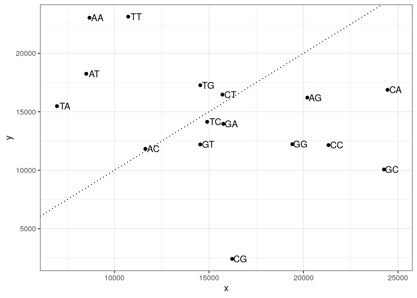
Random Forests
Use Random Forests to train a predictor using the TSSs and random di-nucleotide frequencies.
load_package('randomForest', source = "cran")Installing package into '/packages'
(as 'lib' is unspecified)randomForest 4.7-1Type rfNews() to see new features/changes/bug fixes.
Attaching package: 'randomForest'The following object is masked from 'package:BiocGenerics':
combineThe following object is masked from 'package:dplyr':
combineThe following object is masked from 'package:ggplot2':
marginCombine TSS and random data.
as.data.frame(my_tss_di) %>%
  mutate(class = 'tss') -> my_data

as.data.frame(my_random_di) %>%
  mutate(class = 'random') %>%
  rbind(my_data) %>%
  mutate(class = factor(class)) -> my_data

dim(my_data)
[1] 120882 17Split 80/20.
set.seed(1984)
idx <- sample(nrow(my_data), nrow(my_data)*0.8)

train <- my_data[idx, ]
test <- my_data[-idx, ]

dim(train)
[1] 96705 17dim(test)[1] 24177 17Train Random Forest.
r <- randomForest(
  class ~ .,
  data = train,
  importance = TRUE,
  do.trace=100
)
ntree OOB 1 2
100: 26.90% 27.00% 26.81%
200: 26.83% 27.04% 26.63%
300: 26.79% 26.87% 26.72%
400: 26.76% 26.86% 26.67%
500: 26.73% 26.91% 26.57%r
Call:
 randomForest(formula = class ~ ., data = train, importance = TRUE,      do.trace = 100)
               Type of random forest: classification
                     Number of trees: 500
No. of variables tried at each split: 4

        OOB estimate of  error rate: 26.73%
Confusion matrix:
       random   tss class.error
random  34411 12671   0.2691262
tss     13183 36440   0.2656631
Feature importance.
rn <- round(importance(r), 2)
rn[order(rn[,3], decreasing=TRUE),]
random tss MeanDecreaseAccuracy MeanDecreaseGini
AA 36.97 62.60 83.80 1453.94
AT -1.20 68.43 77.04 944.30
CA -43.86 72.19 76.41 881.85
AC -1.99 53.47 73.54 449.49
GG -3.29 56.13 72.93 481.68
CG 61.48 52.18 70.53 2674.33
TG 10.48 50.81 68.65 530.84
CT 24.31 42.48 65.64 470.32
TT 17.16 51.34 62.09 1049.67
GT 15.32 39.77 59.68 417.05
AG -17.12 49.23 59.49 516.90
GA -23.64 51.40 59.05 401.20
CC 1.55 52.68 56.29 703.49
TA -18.74 51.20 52.40 643.57
GC 29.91 39.93 51.43 1024.63
TC 15.88 33.00 49.70 427.67As a plot.
varImpPlot(r)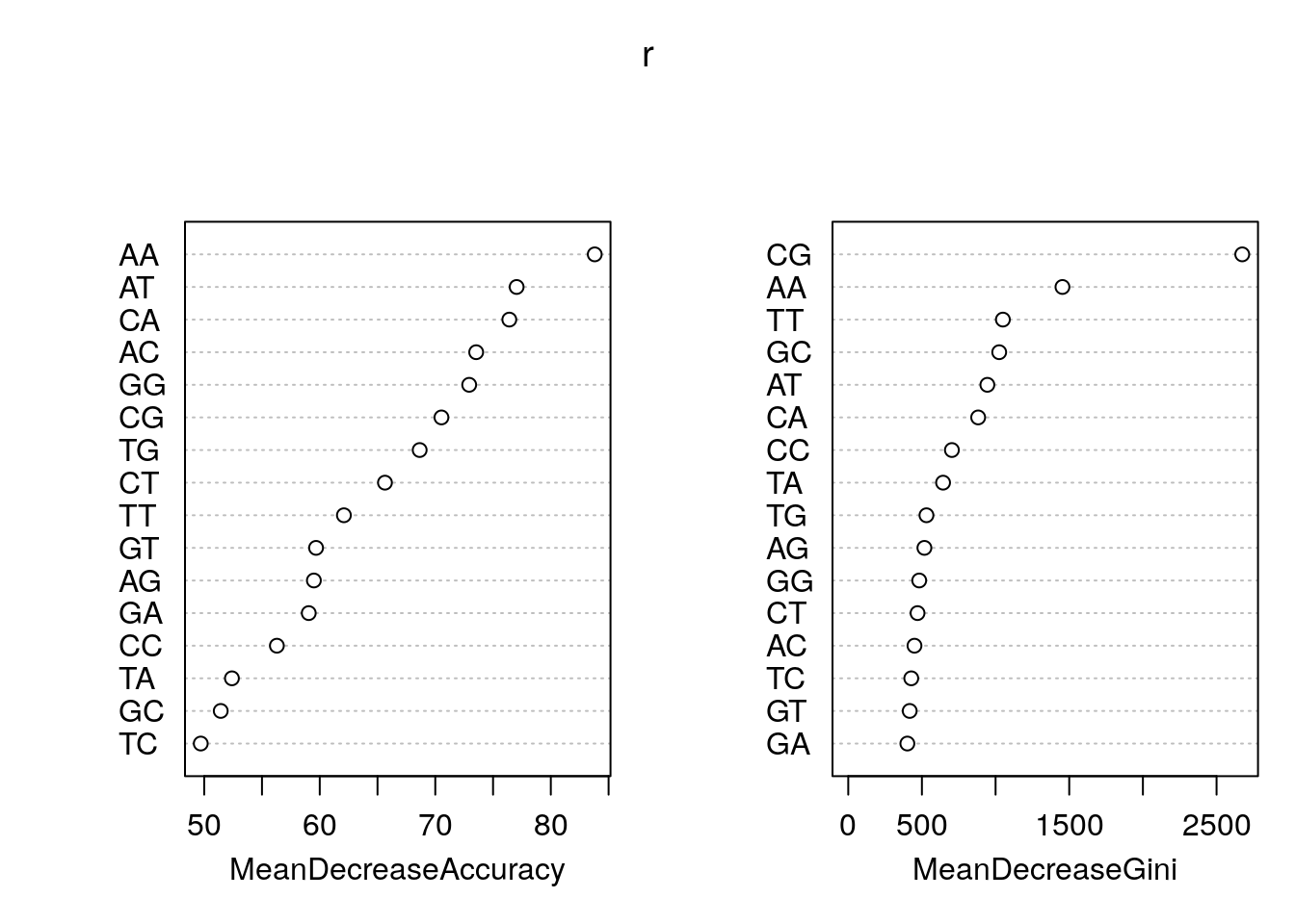
Predict.
data.predict <- predict(r, test)
prop.table(table(observed = test$class, predict = data.predict), 1)
predict
observed random tss
random 0.7229678 0.2770322
tss 0.2617194 0.7382806Use pROC package to get area under curve.
load_package("pROC", source = "cran")Check ROC.
roc(r$y, r$votes[, 'random'])Setting levels: control = random, case = tssSetting direction: controls > cases
Call:
roc.default(response = r$y, predictor = r$votes[, "random"])

Data: r$votes[, "random"] in 47082 controls (r$y random) > 49623 cases (r$y tss).
Area under the curve: 0.7969
Plot ROC with the verification package.
load_package('verification', source = "cran")Plot ROC.
aucc <- roc.area(as.integer(train$class=='tss'), r$votes[,2])$A
roc.plot(as.integer(train$class=='tss'), r$votes[,2], main="")
Warning in roc.plot.default(as.integer(train$class == "tss"), r$votes[, : Large
amount of unique predictions used as thresholds. Consider specifying thresholds.legend("bottomright", bty="n", sprintf("Area Under the Curve (AUC) = %1.3f", aucc))
title(main="OOB ROC Curve Random Forest for predicting TSS")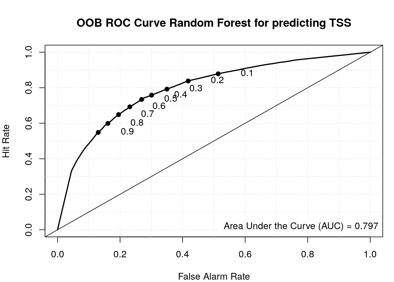
sessionInfo()R version 4.1.2 (2021-11-01)
Platform: x86_64-pc-linux-gnu (64-bit)
Running under: Ubuntu 20.04.3 LTS
Matrix products: default
BLAS/LAPACK: /usr/lib/x86_64-linux-gnu/openblas-pthread/libopenblasp-r0.3.8.so
locale:
[1] LC_CTYPE=en_US.UTF-8 LC_NUMERIC=C
[3] LC_TIME=en_US.UTF-8 LC_COLLATE=en_US.UTF-8
[5] LC_MONETARY=en_US.UTF-8 LC_MESSAGES=en_US.UTF-8
[7] LC_PAPER=en_US.UTF-8 LC_NAME=C
[9] LC_ADDRESS=C LC_TELEPHONE=C
[11] LC_MEASUREMENT=en_US.UTF-8 LC_IDENTIFICATION=C
attached base packages:
[1] stats4 stats graphics grDevices utils datasets methods
[8] base
other attached packages:
[1] verification_1.42 dtw_1.22-3
[3] proxy_0.4-26 CircStats_0.2-6
[5] MASS_7.3-54 boot_1.3-28
[7] fields_13.3 viridis_0.6.2
[9] viridisLite_0.4.0 spam_2.8-0
[11] pROC_1.18.0 randomForest_4.7-1
[13] BSgenome.Hsapiens.UCSC.hg38_1.4.4 BSgenome_1.62.0
[15] rtracklayer_1.54.0 Biostrings_2.62.0
[17] XVector_0.34.0 GenomicRanges_1.46.1
[19] GenomeInfoDb_1.30.1 IRanges_2.28.0
[21] S4Vectors_0.32.4 BiocGenerics_0.40.0
[23] biomaRt_2.50.3 forcats_0.5.1
[25] stringr_1.4.0 dplyr_1.0.8
[27] purrr_0.3.4 readr_2.1.2
[29] tidyr_1.2.0 tibble_3.1.6
[31] ggplot2_3.3.5 tidyverse_1.3.1
[33] workflowr_1.7.0
loaded via a namespace (and not attached):
[1] readxl_1.4.0 backports_1.4.1
[3] BiocFileCache_2.2.1 plyr_1.8.7
[5] BiocParallel_1.28.3 digest_0.6.29
[7] htmltools_0.5.2 fansi_1.0.3
[9] magrittr_2.0.3 memoise_2.0.1
[11] tzdb_0.3.0 modelr_0.1.8
[13] matrixStats_0.62.0 prettyunits_1.1.1
[15] colorspace_2.0-3 blob_1.2.3
[17] rvest_1.0.2 rappdirs_0.3.3
[19] haven_2.5.0 xfun_0.30
[21] callr_3.7.0 crayon_1.5.1
[23] RCurl_1.98-1.6 jsonlite_1.8.0
[25] glue_1.6.2 gtable_0.3.0
[27] zlibbioc_1.40.0 DelayedArray_0.20.0
[29] maps_3.4.0 scales_1.2.0
[31] DBI_1.1.2 Rcpp_1.0.8.3
[33] progress_1.2.2 bit_4.0.4
[35] dotCall64_1.0-1 httr_1.4.2
[37] ellipsis_0.3.2 pkgconfig_2.0.3
[39] XML_3.99-0.9 farver_2.1.0
[41] sass_0.4.1 dbplyr_2.1.1
[43] utf8_1.2.2 tidyselect_1.1.2
[45] labeling_0.4.2 rlang_1.0.2
[47] later_1.3.0 AnnotationDbi_1.56.2
[49] munsell_0.5.0 cellranger_1.1.0
[51] tools_4.1.2 cachem_1.0.6
[53] cli_3.2.0 generics_0.1.2
[55] RSQLite_2.2.12 broom_0.8.0
[57] evaluate_0.15 fastmap_1.1.0
[59] yaml_2.3.5 processx_3.5.3
[61] knitr_1.38 bit64_4.0.5
[63] fs_1.5.2 KEGGREST_1.34.0
[65] whisker_0.4 xml2_1.3.3
[67] compiler_4.1.2 rstudioapi_0.13
[69] filelock_1.0.2 curl_4.3.2
[71] png_0.1-7 reprex_2.0.1
[73] bslib_0.3.1 stringi_1.7.6
[75] highr_0.9 ps_1.6.0
[77] lattice_0.20-45 Matrix_1.3-4
[79] vctrs_0.4.1 pillar_1.7.0
[81] lifecycle_1.0.1 BiocManager_1.30.16
[83] jquerylib_0.1.4 bitops_1.0-7
[85] httpuv_1.6.5 R6_2.5.1
[87] BiocIO_1.4.0 promises_1.2.0.1
[89] gridExtra_2.3 assertthat_0.2.1
[91] SummarizedExperiment_1.24.0 rprojroot_2.0.3
[93] rjson_0.2.21 withr_2.5.0
[95] GenomicAlignments_1.30.0 Rsamtools_2.10.0
[97] GenomeInfoDbData_1.2.7 parallel_4.1.2
[99] hms_1.1.1 grid_4.1.2
[101] rmarkdown_2.13 MatrixGenerics_1.6.0
[103] git2r_0.30.1 getPass_0.2-2
[105] Biobase_2.54.0 lubridate_1.8.0
[107] restfulr_0.0.13