Mutated gene analysis across all lines
Davis J. McCarthy
Last updated: 2018-08-25
workflowr checks: (Click a bullet for more information)-
✔ R Markdown file: up-to-date
Great! Since the R Markdown file has been committed to the Git repository, you know the exact version of the code that produced these results.
-
✔ Environment: empty
Great job! The global environment was empty. Objects defined in the global environment can affect the analysis in your R Markdown file in unknown ways. For reproduciblity it’s best to always run the code in an empty environment.
-
✔ Seed:
set.seed(20180807)The command
set.seed(20180807)was run prior to running the code in the R Markdown file. Setting a seed ensures that any results that rely on randomness, e.g. subsampling or permutations, are reproducible. -
✔ Session information: recorded
Great job! Recording the operating system, R version, and package versions is critical for reproducibility.
-
Great! You are using Git for version control. Tracking code development and connecting the code version to the results is critical for reproducibility. The version displayed above was the version of the Git repository at the time these results were generated.✔ Repository version: a865fa3
Note that you need to be careful to ensure that all relevant files for the analysis have been committed to Git prior to generating the results (you can usewflow_publishorwflow_git_commit). workflowr only checks the R Markdown file, but you know if there are other scripts or data files that it depends on. Below is the status of the Git repository when the results were generated:
Note that any generated files, e.g. HTML, png, CSS, etc., are not included in this status report because it is ok for generated content to have uncommitted changes.Ignored files: Ignored: .DS_Store Ignored: .Rhistory Ignored: .Rproj.user/ Ignored: .vscode/ Ignored: code/.DS_Store Ignored: data/raw/ Ignored: src/.DS_Store Ignored: src/.ipynb_checkpoints/ Ignored: src/Rmd/.Rhistory Untracked files: Untracked: Snakefile_clonality Untracked: Snakefile_somatic_calling Untracked: code/analysis_for_garx.Rmd Untracked: code/selection/ Untracked: code/yuanhua/ Untracked: data/canopy/ Untracked: data/cell_assignment/ Untracked: data/de_analysis_FTv62/ Untracked: data/donor_info_070818.txt Untracked: data/donor_info_core.csv Untracked: data/donor_neutrality.tsv Untracked: data/exome-point-mutations/ Untracked: data/fdr10.annot.txt.gz Untracked: data/human_H_v5p2.rdata Untracked: data/human_c2_v5p2.rdata Untracked: data/human_c6_v5p2.rdata Untracked: data/neg-bin-rsquared-petr.csv Untracked: data/neutralitytestr-petr.tsv Untracked: data/sce_merged_donors_cardelino_donorid_all_qc_filt.rds Untracked: data/sce_merged_donors_cardelino_donorid_all_with_qc_labels.rds Untracked: data/sce_merged_donors_cardelino_donorid_unstim_qc_filt.rds Untracked: data/sces/ Untracked: data/selection/ Untracked: data/simulations/ Untracked: data/variance_components/ Untracked: docs/figure/selection_models.Rmd/ Untracked: figures/ Untracked: output/differential_expression/ Untracked: output/donor_specific/ Untracked: output/line_info.tsv Untracked: output/nvars_by_category_by_donor.tsv Untracked: output/nvars_by_category_by_line.tsv Untracked: output/variance_components/ Untracked: references/ Untracked: tree.txt
Expand here to see past versions:
| File | Version | Author | Date | Message |
|---|---|---|---|---|
| Rmd | d618fe5 | davismcc | 2018-08-25 | Updating analyses |
| html | 090c1b9 | davismcc | 2018-08-24 | Build site. |
| html | d2e8b31 | davismcc | 2018-08-19 | Build site. |
| html | 1489d32 | davismcc | 2018-08-17 | Add html files |
| Rmd | d5e785d | davismcc | 2018-08-17 | Updating to use “line” instead of “donor” |
| Rmd | bcee02b | davismcc | 2018-08-17 | Updating donors to lines in text. |
| Rmd | 0862ede | davismcc | 2018-08-10 | Fixing some typos |
| Rmd | a27cace | davismcc | 2018-08-10 | Updating analysis |
| Rmd | 0c8f70d | davismcc | 2018-08-10 | Tidying up mutated genes analysis |
| Rmd | 1cbadbd | davismcc | 2018-08-10 | Updating analyses. |
| Rmd | de1daa9 | davismcc | 2018-08-09 | Adding analysis for DE between mutated and unmutated clones |
Introduction
In this analysis, we look at the direct impact of somatic variants on the genes in which they are located. We combine information from the clonal trees about which variants tag which clones and VEP functional annotations about the expected consequence of each variant. For each gene with a somatic variant (and sufficient gene expression), we test for differential expression between cells that have the mutation (based on clone assignment) and those that do not. We can then compare these “mutated gene” differential expression results for variants with different categories of functional annotation.
Clonal trees were inferred with Canopy using variant allele frequency information from a set of strictly filtered somatic variants called from whole-exome sequencing data. We filtered somatic variants to only include variants that had read coverage in at least one single-cell for the relevant line. Assignment of cells to clones was done with cardelino.
Load libraries and data
Load VEP consequence information.
vep_best <- read_tsv("data/exome-point-mutations/high-vs-low-exomes.v62.ft.alldonors-filt_lenient.all_filt_sites.vep_most_severe_csq.txt")
colnames(vep_best)[1] <- "Uploaded_variation"
## deduplicate dataframe
vep_best <- vep_best[!duplicated(vep_best[["Uploaded_variation"]]),]
There are 8503 variants, aggregated across all lines, and we can check the number that fall into the different VEP annotation categories.
table(vep_best[["Consequence"]])
               3_prime_UTR_variant                5_prime_UTR_variant
                               181                                121
           downstream_gene_variant                 intergenic_variant
                                13                                 13
                    intron_variant               mature_miRNA_variant
                              1539                                  3
                  missense_variant non_coding_transcript_exon_variant
                              3648                                428
         regulatory_region_variant            splice_acceptor_variant
                                 1                                 41
              splice_donor_variant              splice_region_variant
                                24                                291
                        start_lost                        stop_gained
                                 9                                227
                         stop_lost              stop_retained_variant
                                 2                                  5
                synonymous_variant              upstream_gene_variant
                              1923                                 34
Load exome sites, that is, the somatic SNVs identified with Petr Danecek’s somatic variant calling approach.
exome_sites <- read_tsv("data/exome-point-mutations/high-vs-low-exomes.v62.ft.filt_lenient-alldonors.txt.gz",
    col_types = "ciccdcciiiiccccccccddcdcll", comment = "#",
    col_names = TRUE)
exome_sites <- dplyr::select(exome_sites,
                             -c(clinsing, SIFT_Pdel, PolyPhen_Pdel, gene_name,
                                bcftools_csq))
exome_sites <- dplyr::mutate(
    exome_sites,
    chrom = paste0("chr", gsub("chr", "", chrom)),
    var_id = paste0(chrom, ":", pos, "_", ref, "_", alt))
## deduplicate sites list
exome_sites <- exome_sites[!duplicated(exome_sites[["var_id"]]),]
Add variant consequences annotations to exome sites.
vep_best[["var_id"]] <- paste0("chr", vep_best[["Uploaded_variation"]])
vep_best[, c("var_id", "Location", "Consequence")]
# A tibble: 8,503 x 3
var_id Location Consequence
<chr> <chr> <chr>
1 chr1:874501_C_T 1:874501-874501 missense_variant
2 chr1:915025_G_A 1:915025-915025 missense_variant
3 chr1:916622_C_T 1:916622-916622 intron_variant
4 chr1:985731_G_A 1:985731-985731 intron_variant
5 chr1:985732_G_A 1:985732-985732 intron_variant
6 chr1:1019508_G_A 1:1019508-1019508 missense_variant
7 chr1:1019509_G_A 1:1019509-1019509 synonymous_variant
8 chr1:1116160_G_A 1:1116160-1116160 synonymous_variant
9 chr1:1158664_G_A 1:1158664-1158664 synonymous_variant
10 chr1:1178463_T_A 1:1178463-1178463 missense_variant
# ... with 8,493 more rowsexome_sites <- inner_join(exome_sites,
vep_best[, c("var_id", "Location", "Consequence")],
by = "var_id")
# com_vars <- intersect(exome_sites$var_id, csq_annos$var_id)
# length(com_vars)
# mean(exome_sites$var_id %in% csq_annos$var_id)
# mean(exome_sites$pos %in% csq_annos$Pos)Load SingleCellExperiment objects with single-cell gene expression data.
params <- list()
params$callset <- "filt_lenient.cell_coverage_sites"
fls <- list.files("data/sces")
fls <- fls[grepl(params$callset, fls)]
lines <- gsub(".*ce_([a-z]+)_.*", "\\1", fls)

sce_unst_list <- list()
for (don in lines) {
    sce_unst_list[[don]] <- readRDS(file.path("data/sces",
        paste0("sce_", don, "_with_clone_assignments.", params$callset, ".rds")))
    cat(paste("reading", don, ":   ", ncol(sce_unst_list[[don]]), "cells.\n"))
}
reading euts : 79 cells.
reading fawm : 53 cells.
reading feec : 75 cells.
reading fikt : 39 cells.
reading garx : 70 cells.
reading gesg : 105 cells.
reading heja : 50 cells.
reading hipn : 62 cells.
reading ieki : 58 cells.
reading joxm : 79 cells.
reading kuco : 48 cells.
reading laey : 55 cells.
reading lexy : 63 cells.
reading naju : 44 cells.
reading nusw : 60 cells.
reading oaaz : 38 cells.
reading oilg : 90 cells.
reading pipw : 107 cells.
reading puie : 41 cells.
reading qayj : 97 cells.
reading qolg : 36 cells.
reading qonc : 58 cells.
reading rozh : 91 cells.
reading sehl : 30 cells.
reading ualf : 89 cells.
reading vass : 37 cells.
reading vils : 37 cells.
reading vuna : 71 cells.
reading wahn : 82 cells.
reading wetu : 77 cells.
reading xugn : 35 cells.
reading zoxy : 88 cells.assignments_lst <- list()
for (don in lines) {
assignments_lst[[don]] <- as_data_frame(
colData(sce_unst_list[[don]])[,
c("donor_short_id", "highest_prob",
"assigned", "total_features",
"total_counts_endogenous", "num_processed")])
}
assignments <- do.call("rbind", assignments_lst)We have SCE objects (expression data and cell assignments) for 32 lines, with 85% of cells confidently assigned to a clone.
Finally, we load transcriptome-wide differential expression results computed using the quasi-likelihood F test method in edgeR.
de_res <- readRDS(paste0("data/de_analysis_FTv62/",
                         params$callset,
                         ".de_results_unstimulated_cells.rds"))
Annotating variants with clone presence by line
Next, we need to annotate the variants with information about which clones they are expected to be present in (obtained from the Canopy tree inference).
cell_assign_list <- list()
for (don in lines) {
    cell_assign_list[[don]] <- readRDS(file.path("data/cell_assignment",
        paste0("cardelino_results.", don, ".", params$callset, ".rds")))
    cat(paste("reading", don, "\n"))
}
reading euts
reading fawm
reading feec
reading fikt
reading garx
reading gesg
reading heja
reading hipn
reading ieki
reading joxm
reading kuco
reading laey
reading lexy
reading naju
reading nusw
reading oaaz
reading oilg
reading pipw
reading puie
reading qayj
reading qolg
reading qonc
reading rozh
reading sehl
reading ualf
reading vass
reading vils
reading vuna
reading wahn
reading wetu
reading xugn
reading zoxy get_sites_by_line <- function(sites_df, sce_list, assign_list) {
if (!identical(sort(names(sce_list)), sort(names(assign_list))))
stop("lines do not match between sce_list and assign_list.")
sites_by_line <- list()
for (don in names(sce_list)) {
config <- as_data_frame(assign_list[[don]]$tree$Z)
config[["var_id"]] <- rownames(assign_list[[don]]$tree$Z)
sites_line <- inner_join(sites_df, config)
sites_line[["clone_presence"]] <- ""
for (cln in colnames(assign_list[[don]]$tree$Z)[-1]) {
sites_line[["clone_presence"]][
as.logical(sites_line[[cln]])] <- paste(
sites_line[["clone_presence"]][
as.logical(sites_line[[cln]])], cln, sep = "&")
}
sites_line[["clone_presence"]] <- gsub("^&", "",
sites_line[["clone_presence"]])
## drop config columns as these won't match up between lines
keep_cols <- grep("^clone[0-9]$", colnames(sites_line), invert = TRUE)
sites_by_line[[don]] <- sites_line[, keep_cols]
}
do.call("bind_rows", sites_by_line)
}
sites_by_line <- get_sites_by_line(exome_sites, sce_unst_list, cell_assign_list)
sites_by_line <- dplyr::mutate(sites_by_line,
Consequence = gsub("_variant", "", Consequence))Differential expression comparing mutated clone to all other clones
Get DE results comparing mutated clone to all unmutated clones, but we first have to organise the data further.
Turn dataframes into GRanges objects to enable fast and robust overlaps.
## run DE for mutated cells vs unmutated cells using existing DE results
## filter out any remaining ERCC genes
for (don in names(de_res[["sce_list_unst"]]))
    de_res[["sce_list_unst"]][[don]] <- de_res[["sce_list_unst"]][[don]][
        !rowData(de_res[["sce_list_unst"]][[don]])$is_feature_control,]
sce_de_list_gr <- list()
for (don in names(de_res[["sce_list_unst"]])) {
    sce_de_list_gr[[don]] <- makeGRangesFromDataFrame(
        rowData(de_res[["sce_list_unst"]][[don]]),
        start.field = "start_position",
        end.field = "end_position",
        keep.extra.columns = TRUE)
    seqlevelsStyle(sce_de_list_gr[[don]]) <- "Ensembl"
}
sites_by_line <- dplyr::mutate(sites_by_line, end_pos = pos)
sites_by_line_gr <- makeGRangesFromDataFrame(
        sites_by_line,
        start.field = "pos",
        end.field = "end_pos",
        keep.extra.columns = TRUE)
seqlevelsStyle(sites_by_line_gr) <- "Ensembl"
Run DE testing between mutated and un-mutated clones for all affected genes for each line.
mut_genes_df_allcells_list <- list()
for (don in names(de_res[["sce_list_unst"]])) {
    cat("working on ", don, "\n")
    sites_tmp <- sites_by_line_gr[sites_by_line_gr$donor_short_id == don]
    ov_tmp <- findOverlaps(sce_de_list_gr[[don]], sites_tmp)
    sce_tmp <- de_res[["sce_list_unst"]][[don]][queryHits(ov_tmp),]
    sites_tmp <- sites_tmp[subjectHits(ov_tmp)]
    sites_tmp$gene <- rownames(sce_tmp)
    dge_tmp <- de_res[["dge_list"]][[don]]
    dge_tmp <- dge_tmp[intersect(rownames(dge_tmp), sites_tmp$gene),]
    base_design <- dge_tmp$design[, !grepl("assigned", colnames(dge_tmp$design))]
    de_tbl_tmp <- data.frame(line = don,
                             gene = sites_tmp$gene,
                             hgnc_symbol = gsub(".*_", "", sites_tmp$gene),
                             ensembl_gene_id = gsub("_.*", "", sites_tmp$gene),
                             var_id = sites_tmp$var_id,
                             location = sites_tmp$Location,
                             consequence = sites_tmp$Consequence,
                             clone_presence = sites_tmp$clone_presence,
                             logFC = NA, logCPM = NA, F = NA, PValue = NA,
                             comment = "", stringsAsFactors = FALSE)
    for (i in seq_len(length(sites_tmp))) {
        clones_tmp <- strsplit(sites_tmp$clone_presence[i], split = "&")[[1]]
        mutatedclone <- as.numeric(sce_tmp$assigned %in% clones_tmp)
        dsgn_tmp <- cbind(base_design, data.frame(mutatedclone))
        if (sites_tmp$gene[i] %in% rownames(dge_tmp) && is.fullrank(dsgn_tmp)) {
            qlfit_tmp <- glmQLFit(dge_tmp[sites_tmp$gene[i],], dsgn_tmp)
            de_tmp <- glmQLFTest(qlfit_tmp, coef = ncol(dsgn_tmp))
            de_tbl_tmp$logFC[i] <- de_tmp$table$logFC
            de_tbl_tmp$logCPM[i] <- de_tmp$table$logCPM
            de_tbl_tmp$F[i] <- de_tmp$table$F
            de_tbl_tmp$PValue[i] <- de_tmp$table$PValue
        }
        if (!(sites_tmp$gene[i] %in% rownames(dge_tmp)))
            de_tbl_tmp$comment[i] <- "gene did not pass DE filters"
        if (!is.fullrank(dsgn_tmp))
            de_tbl_tmp$comment[i] <- "insufficient cells assigned to clone"
    }
    mut_genes_df_allcells_list[[don]] <- de_tbl_tmp
}
working on euts
working on fawm
working on feec
working on fikt
working on garx
working on gesg
working on heja
working on hipn
working on ieki
working on joxm
working on kuco
working on laey
working on lexy
working on naju
working on nusw
working on oaaz
working on oilg
working on pipw
working on puie
working on qayj
working on qolg
working on qonc
working on rozh
working on sehl
working on ualf
working on vass
working on vuna
working on wahn
working on wetu
working on xugn
working on zoxy mut_genes_df_allcells <- do.call("bind_rows", mut_genes_df_allcells_list)
dim(mut_genes_df_allcells)[1] 1140 13head(mut_genes_df_allcells) line gene hgnc_symbol ensembl_gene_id
1 euts ENSG00000006327_TNFRSF12A TNFRSF12A ENSG00000006327
2 euts ENSG00000028528_SNX1 SNX1 ENSG00000028528
3 euts ENSG00000060642_PIGV PIGV ENSG00000060642
4 euts ENSG00000083168_KAT6A KAT6A ENSG00000083168
5 euts ENSG00000083520_DIS3 DIS3 ENSG00000083520
6 euts ENSG00000090060_PAPOLA PAPOLA ENSG00000090060
var_id location consequence clone_presence
1 chr16:3071779_A_T 16:3071779-3071779 stop_gained clone2
2 chr15:64388302_G_A 15:64388302-64388302 synonymous clone3
3 chr1:27121236_G_A 1:27121236-27121236 synonymous clone3
4 chr8:41798596_G_A 8:41798596-41798596 missense clone2
5 chr13:73335940_G_C 13:73335940-73335940 synonymous clone2&clone3
6 chr14:97000841_C_T 14:97000841-97000841 missense clone3
logFC logCPM F PValue
1 0.08487392 9.225735 0.1704411 0.6809820
2 NA NA NA NA
3 NA NA NA NA
4 -0.75250667 3.108107 1.9374726 0.1683502
5 -0.79956030 4.352695 1.1304492 0.2913337
6 NA NA NA NA
comment
1
2 insufficient cells assigned to clone
3 insufficient cells assigned to clone
4
5
6 insufficient cells assigned to cloneWith this analysis, 1011 genes/variants could be tested for DE between mutated and unmutated clones.
We can recompute false discovery rates with IHW, simplify the VEP annotation categories (assigning all nonsense categories to “nonsense” and all splicing categories to “splicing”) and inspect the results.
## add FDRs for genes tested here for DE
ihw_res_all <- ihw(PValue ~ logCPM, data = mut_genes_df_allcells, alpha = 0.2)
mut_genes_df_allcells$FDR <- adj_pvalues(ihw_res_all)
## add simplified consequence categories
mut_genes_df_allcells$consequence_simplified <-
    mut_genes_df_allcells$consequence
mut_genes_df_allcells$consequence_simplified[
    mut_genes_df_allcells$consequence_simplified %in%
        c("stop_retained", "start_lost", "stop_lost", "stop_gained")] <- "nonsense"
mut_genes_df_allcells$consequence_simplified[
    mut_genes_df_allcells$consequence_simplified %in%
        c("splice_donor", "splice_acceptor", "splice_region")] <- "splicing"
table(mut_genes_df_allcells$consequence_simplified)
               3_prime_UTR                5_prime_UTR
                        27                         12
                    intron                   missense
                        20                        650
non_coding_transcript_exon                   nonsense
                        20                         39
                  splicing                 synonymous
21 351 summary(mut_genes_df_allcells$FDR) Min. 1st Qu. Median Mean 3rd Qu. Max. NA's
0.0000 0.5465 0.8892 0.7571 0.9376 0.9972 129 dplyr::arrange(mut_genes_df_allcells, FDR) %>% dplyr::select(-location) %>%
DT::datatable(., options = list(pageLength = 20))There are few variants with a significant difference in expression between clones with and without the mutation (FDR < 10%).
Plot these results.
dplyr::filter(mut_genes_df_allcells, !is.na(logFC)) %>%
ggplot(aes(x = logFC, y = -log10(PValue),
                         fill = FDR < 0.1)) +
    geom_point(colour = "gray40", pch = 21) +
    geom_rug(sides = "b", alpha = 0.6) +
    geom_vline(xintercept = 0, linetype = 2) +
    # geom_text_repel(show.legend = FALSE) +
    scale_fill_manual(values = c("gray70", "firebrick"),
                        label = c("N.S.", "FDR < 10%"),
                        name = "DE result") +
    facet_wrap(~consequence, ncol = 5) +
    guides(alpha = FALSE) +
    theme_classic(16) +
    theme(strip.background = element_rect(fill = "gray90"),
          legend.position = c(0.9, 0.1))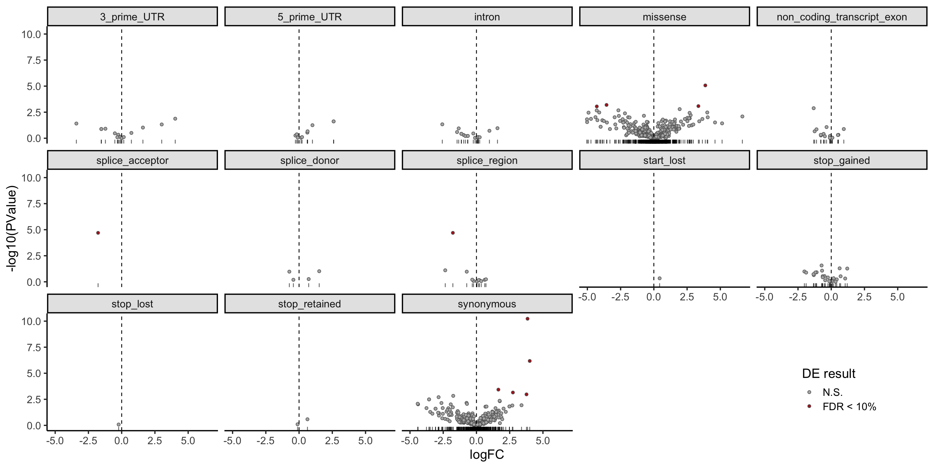
ggsave("figures/mutated_genes/alllines_mutgenes_volcano_by_vep_anno_allcells.png",
       height = 7, width = 16)
ggsave("figures/mutated_genes/alllines_mutgenes_volcano_by_vep_anno_allcells.pdf",
       height = 7, width = 16)
ggsave("figures/mutated_genes/alllines_mutgenes_volcano_by_vep_anno_allcells.svg",
       height = 7, width = 16)
The picture can look a little clearer with simplified annotation categories.
dplyr::filter(mut_genes_df_allcells, !is.na(logFC)) %>%
ggplot(aes(x = logFC, y = -log10(PValue),
                         fill = FDR < 0.2)) +
    geom_point(colour = "gray40", pch = 21) +
    geom_rug(sides = "b", alpha = 0.6) +
    geom_vline(xintercept = 0, linetype = 2) +
    # geom_text_repel(show.legend = FALSE) +
    scale_fill_manual(values = c("gray70", "firebrick"),
                        label = c("N.S.", "FDR < 20%"),
                        name = "DE result") +
    facet_wrap(~consequence_simplified, ncol = 3) +
    guides(alpha = FALSE) +
    theme_classic(20) +
    theme(strip.background = element_rect(fill = "gray90"),
          strip.text = element_text(size = 13),
          legend.position = c(0.8, 0.15))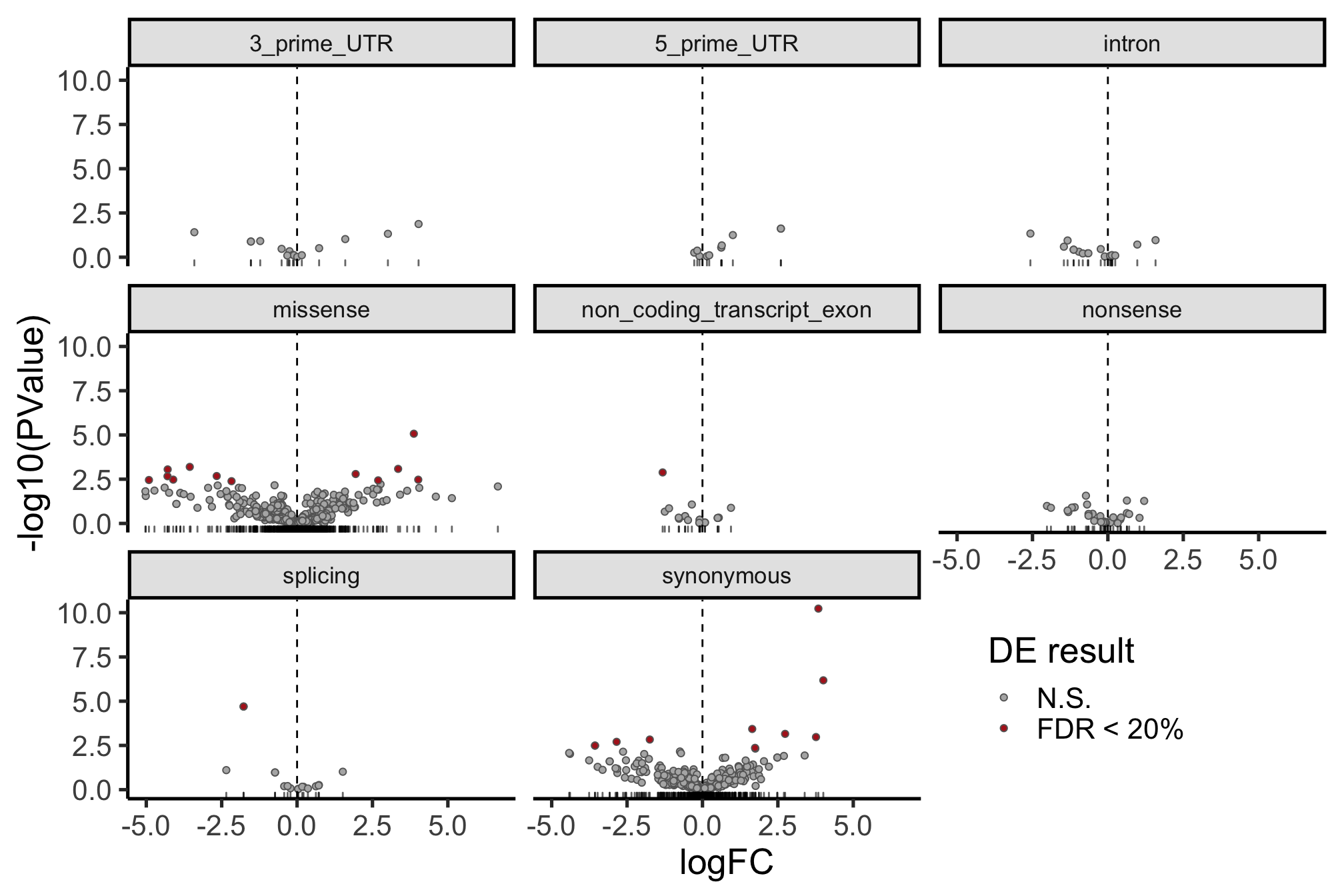
Expand here to see past versions of unnamed-chunk-8-1.png:
| Version | Author | Date |
|---|---|---|
| d2e8b31 | davismcc | 2018-08-19 |
ggsave("figures/mutated_genes/alllines_mutgenes_volcano_by_simple_vep_anno_allcells.png",
       height = 7, width = 10.5)
ggsave("figures/mutated_genes/alllines_mutgenes_volcano_by_simple_vep_anno_allcells.pdf",
       height = 7, width = 10.5)
ggsave("figures/mutated_genes/alllines_mutgenes_volcano_by_simple_vep_anno_allcells.svg",
       height = 7, width = 10.5)
Let us check the median logFC values for each simplified VEP annotation category and add boxplots for logFC to the volcano plots.
tmp2 <- mut_genes_df_allcells %>%
    group_by(consequence_simplified) %>%
    summarise(med = median(logFC, na.rm = TRUE),
              nvars = n())
dplyr::arrange(tmp2, med)
# A tibble: 8 x 3
consequence_simplified med nvars
<chr> <dbl> <int>
1 intron -0.236 20
2 3_prime_UTR -0.193 27
3 nonsense -0.154 39
4 non_coding_transcript_exon -0.106 20
5 synonymous -0.0459 351
6 missense 0.0228 650
7 splicing 0.0355 21
8 5_prime_UTR 0.624 12plist <- list()
simple_cons_vec <- c("nonsense", "splicing", "missense",
"synonymous", "intron",
"non_coding_transcript_exon",
"5_prime_UTR", "3_prime_UTR")
for (cons in simple_cons_vec) {
p <- dplyr::filter(mut_genes_df_allcells, !is.na(logFC),
consequence_simplified == cons) %>%
ggplot(aes(x = logFC, y = -log10(PValue),
fill = FDR < 0.2)) +
geom_point(colour = "gray40", pch = 21, size = 2) +
geom_rug(sides = "b", alpha = 0.6) +
geom_vline(xintercept = 0, linetype = 2) +
scale_fill_manual(values = c("gray70", "firebrick"),
label = c("N.S.", "FDR < 20%"),
name = "DE result") +
guides(alpha = FALSE) +
theme_classic(14) +
ggtitle(cons) +
xlim(1.05 * range(mut_genes_df_allcells$logFC, na.rm = TRUE)) +
ylim(c(0, 1.05 * max(-log10(mut_genes_df_allcells$PValue), na.rm = TRUE))) +
theme(strip.background = element_rect(fill = "gray90"),
strip.text = element_text(size = 12),
legend.position = "none",
plot.title = element_text(face = "bold"))
plist[[cons]] <- ggExtra::ggMarginal(
p, type = "boxplot", margins = "x", fill = "wheat",
colour = "firebrick4", outlier.size = 0, outlier.alpha = 0)
}
cowplot::plot_grid(plotlist = plist, nrow = 2)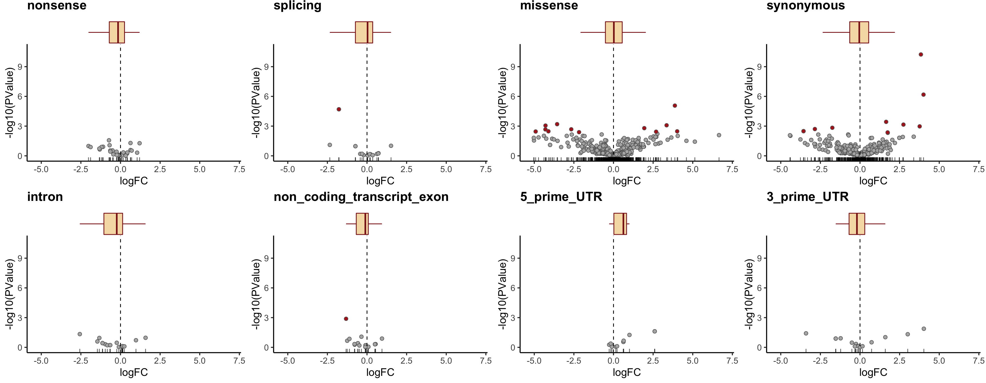
Expand here to see past versions of unnamed-chunk-9-1.png:
| Version | Author | Date |
|---|---|---|
| d2e8b31 | davismcc | 2018-08-19 |
ggsave("figures/mutated_genes/alllines_mutgenes_volcano_by_simple_vep_anno_allcells_with_boxplot.png",
       height = 7, width = 18)
ggsave("figures/mutated_genes/alllines_mutgenes_volcano_by_simple_vep_anno_allcells_with_boxplot.pdf",
       height = 7, width = 18)
ggsave("figures/mutated_genes/alllines_mutgenes_volcano_by_simple_vep_anno_allcells_with_boxplot.svg",
       height = 7, width = 18)
tmp2 <- mut_genes_df_allcells %>%
group_by(consequence) %>%
summarise(med = median(logFC, na.rm = TRUE),
nvars = n())
mut_genes_df_allcells %>%
dplyr::filter(!is.na(logFC)) %>%
dplyr::mutate(consequence = factor(
consequence, levels(as.factor(consequence))[order(tmp2[["med"]])]),
de = ifelse(FDR < 0.2, "FDR < 0.2", "FDR > 0.2")) %>%
ggplot(aes(y = logFC, x = consequence)) +
geom_hline(yintercept = 0, linetype = 1, colour = "black") +
ggbeeswarm::geom_quasirandom(colour = "gray40", fill = "gray70", pch = 21) +
geom_boxplot(outlier.size = 0, outlier.alpha = 0, fill = "wheat",
colour = "firebrick4", width = 0.2, size = 1) +
scale_x_discrete(expand = c(.01, 0)) +
scale_y_continuous(expand = c(0, 0), name = "logFC") +
theme_ridges(16) +
coord_flip() +
theme(strip.background = element_rect(fill = "gray90")) +
guides(fill = FALSE, color = FALSE, point_color = FALSE)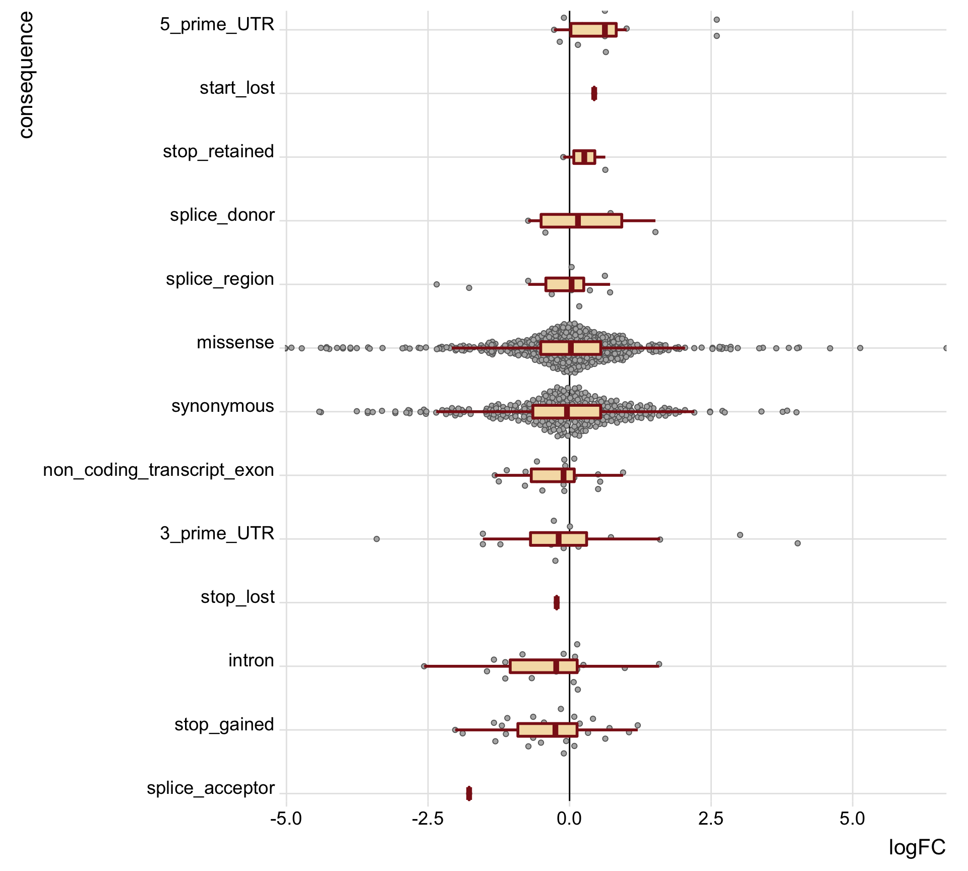
Expand here to see past versions of unnamed-chunk-10-1.png:
| Version | Author | Date |
|---|---|---|
| d2e8b31 | davismcc | 2018-08-19 |
ggsave("figures/mutated_genes/alllines_mutgenes_logfc-box_by_vep_anno_allcells.png",
       height = 9, width = 10)
ggsave("figures/mutated_genes/alllines_mutgenes_logfc-box_by_vep_anno_allcells.pdf",
       height = 9, width = 10)
ggsave("figures/mutated_genes/alllines_mutgenes_logfc-box_by_vep_anno_allcells.svg",
       height = 9, width = 10)
We can also just look specifically at the boxplots of the logFC values across categories, first looking at the median logFC values and results from a t-test testing if the mean logFC value is different from zero. Positive logFC values indicate higher expression in the mutated clone, and negative logFC values lower expression in the mutated clone.
tmp3 <- mut_genes_df_allcells %>%
    group_by(consequence_simplified) %>%
    summarise(med = median(logFC, na.rm = TRUE),
              nvars = n(),
              t_coef = t.test(logFC, mu = 0)$estimate,
              t_stat = t.test(logFC, mu = 0)$statistic,
              t_pval = t.test(logFC, mu = 0)$p.value)
tmp3
# A tibble: 8 x 6
consequence_simplified med nvars t_coef t_stat t_pval
<chr> <dbl> <int> <dbl> <dbl> <dbl>
1 3_prime_UTR -0.193 27 0.0147 0.0332 0.974
2 5_prime_UTR 0.624 12 0.720 2.36 0.0397
3 intron -0.236 20 -0.405 -1.87 0.0781
4 missense 0.0228 650 -0.0411 -0.775 0.439
5 non_coding_transcript_exon -0.106 20 -0.260 -1.79 0.0908
6 nonsense -0.154 39 -0.287 -1.99 0.0558
7 splicing 0.0355 21 -0.231 -0.945 0.359
8 synonymous -0.0459 351 -0.112 -1.58 0.116 mut_genes_df_allcells %>%
dplyr::filter(!is.na(logFC)) %>%
dplyr::mutate(consequence_simplified = factor(
consequence_simplified,
levels(as.factor(consequence_simplified))[order(tmp3[["med"]])]),
de = ifelse(FDR < 0.2, "FDR < 0.2", "FDR > 0.2")) %>%
ggplot(aes(y = logFC, x = consequence_simplified)) +
geom_hline(yintercept = 0, linetype = 1, colour = "black") +
ggbeeswarm::geom_quasirandom(colour = "gray40", fill = "gray70", pch = 21) +
geom_boxplot(outlier.size = 0, outlier.alpha = 0, fill = "wheat",
colour = "firebrick4", width = 0.2, size = 1) +
scale_x_discrete(expand = c(.01, 0), name = "consequence") +
scale_y_continuous(expand = c(0, 0), name = "logFC") +
theme_ridges(20) +
coord_flip() +
theme(strip.background = element_rect(fill = "gray90")) +
guides(fill = FALSE, color = FALSE, point_color = FALSE)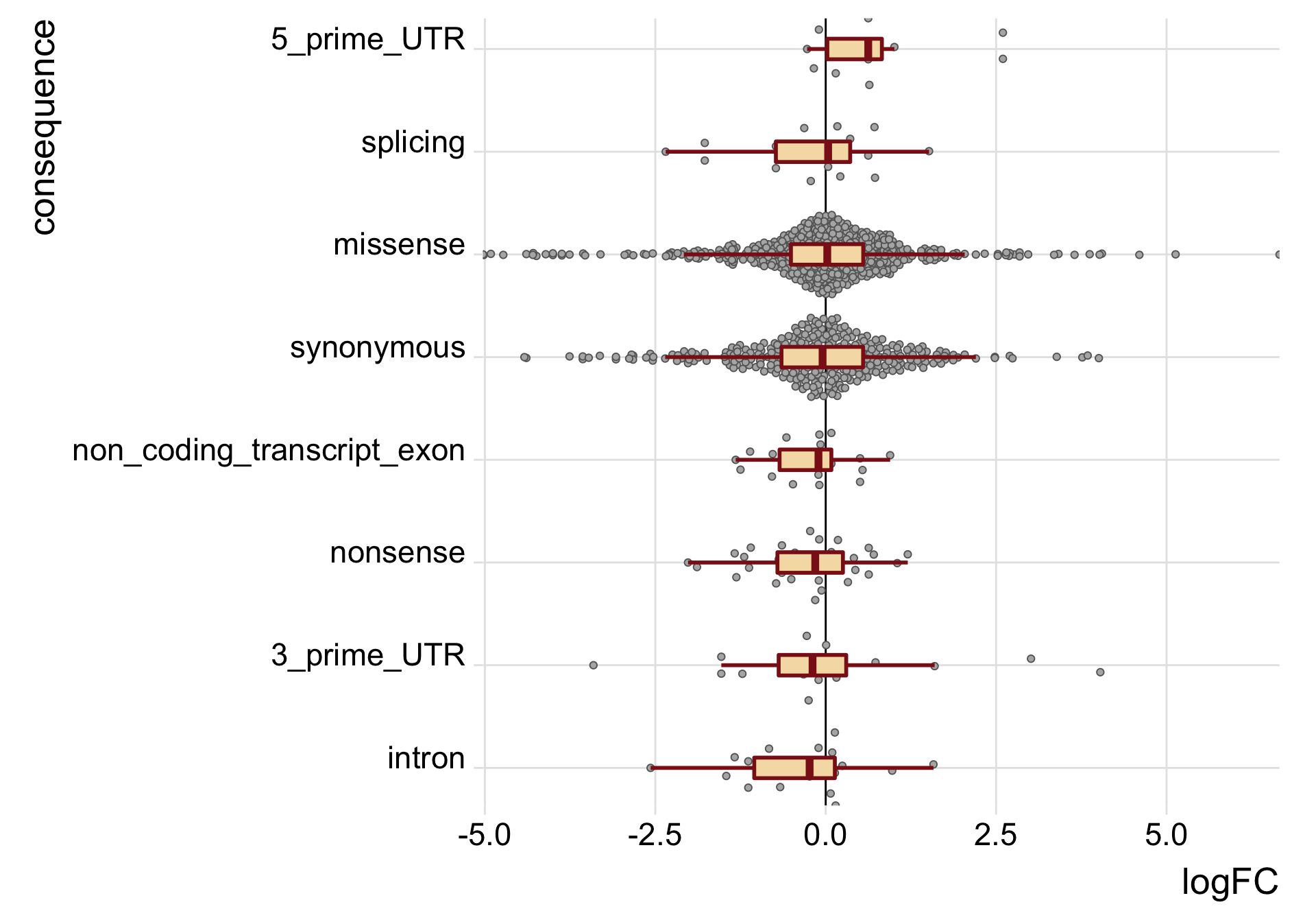
Expand here to see past versions of unnamed-chunk-11-1.png:
| Version | Author | Date |
|---|---|---|
| d2e8b31 | davismcc | 2018-08-19 |
ggsave("figures/mutated_genes/alllines_mutgenes_logfc-box_by_simple_vep_anno_allcells.png",
       height = 7, width = 10)
ggsave("figures/mutated_genes/alllines_mutgenes_logfc-box_by_simple_vep_anno_allcells.pdf",
       height = 7, width = 10)
ggsave("figures/mutated_genes/alllines_mutgenes_logfc-box_by_simple_vep_anno_allcells.svg",
       height = 7, width = 10)
DE for mutated clone: stricter filtering
In the analysis above, the minimum allowed clone size (i.e. group for DE analysis) was 3 cells. Such potentially small group sizes could lead to noisy estimates of the logFC values that we looked at above. Let us repeat the above analysis but increasing the minimum number of cells for a group to 10 to try to obtain more accurate (on average) logFC estimates from the DE model.
Run DE testing between mutated and un-mutated clones for a more strictly filtered set of affected genes for each line.
mut_genes_df_allcells_filt_list <- list()
for (don in names(de_res[["sce_list_unst"]])) {
  cat("working on ", don, "\n")
  sites_tmp <- sites_by_line_gr[sites_by_line_gr$donor_short_id == don]
  ov_tmp <- findOverlaps(sce_de_list_gr[[don]], sites_tmp)
  sce_tmp <- de_res[["sce_list_unst"]][[don]][queryHits(ov_tmp),]
  sites_tmp <- sites_tmp[subjectHits(ov_tmp)]
  sites_tmp$gene <- rownames(sce_tmp)
  dge_tmp <- de_res[["dge_list"]][[don]]
  dge_tmp <- dge_tmp[intersect(rownames(dge_tmp), sites_tmp$gene),]
  base_design <- dge_tmp$design[, !grepl("assigned", colnames(dge_tmp$design))]
  de_tbl_tmp <- data.frame(line = don,
                           gene = sites_tmp$gene,
                           hgnc_symbol = gsub(".*_", "", sites_tmp$gene),
                           ensembl_gene_id = gsub("_.*", "", sites_tmp$gene),
                           var_id = sites_tmp$var_id,
                           location = sites_tmp$Location,
                           consequence = sites_tmp$Consequence,
                           clone_presence = sites_tmp$clone_presence,
                           logFC = NA, logCPM = NA, F = NA, PValue = NA,
                           comment = "", stringsAsFactors = FALSE)
  for (i in seq_len(length(sites_tmp))) {
    clones_tmp <- strsplit(sites_tmp$clone_presence[i], split = "&")[[1]]
    mutatedclone <- as.numeric(sce_tmp$assigned %in% clones_tmp)
    dsgn_tmp <- cbind(base_design, data.frame(mutatedclone))
    if (sites_tmp$gene[i] %in% rownames(dge_tmp) && is.fullrank(dsgn_tmp)
        && (sum(mutatedclone) > 9.5) && (sum(!mutatedclone) > 9.5)) {
      qlfit_tmp <- glmQLFit(dge_tmp[sites_tmp$gene[i],], dsgn_tmp)
      de_tmp <- glmQLFTest(qlfit_tmp, coef = ncol(dsgn_tmp))
      de_tbl_tmp$logFC[i] <- de_tmp$table$logFC
      de_tbl_tmp$logCPM[i] <- de_tmp$table$logCPM
      de_tbl_tmp$F[i] <- de_tmp$table$F
      de_tbl_tmp$PValue[i] <- de_tmp$table$PValue
    }
    if ((sum(mutatedclone) < 9.5) || (sum(!mutatedclone) < 9.5))
      de_tbl_tmp$comment[i] <- "minimum group size < 10 cells"
    if (!(sites_tmp$gene[i] %in% rownames(dge_tmp)))
      de_tbl_tmp$comment[i] <- "gene did not pass DE filters"
    if (!is.fullrank(dsgn_tmp))
      de_tbl_tmp$comment[i] <- "insufficient cells assigned to clone"
  }
  mut_genes_df_allcells_filt_list[[don]] <- de_tbl_tmp
}
working on euts
working on fawm
working on feec
working on fikt
working on garx
working on gesg
working on heja
working on hipn
working on ieki
working on joxm
working on kuco
working on laey
working on lexy
working on naju
working on nusw
working on oaaz
working on oilg
working on pipw
working on puie
working on qayj
working on qolg
working on qonc
working on rozh
working on sehl
working on ualf
working on vass
working on vuna
working on wahn
working on wetu
working on xugn
working on zoxy mut_genes_df_allcells_filt <- do.call("bind_rows", mut_genes_df_allcells_filt_list)With this analysis, 766 could be tested for DE between mutated and unmutated clones (245 fewer than with the lenient filtering above).
We can recompute false discovery rates with IHW, simplify the VEP annotation categories (assigning all nonsense categories to “nonsense” and all splicing categories to “splicing”) and inspect the results.
## add FDRs for genes tested here for DE
ihw_res_all <- ihw(PValue ~ logCPM, data = mut_genes_df_allcells_filt, alpha = 0.2)
mut_genes_df_allcells_filt$FDR <- adj_pvalues(ihw_res_all)
## add simplified consequence categories
mut_genes_df_allcells_filt$consequence_simplified <-
    mut_genes_df_allcells_filt$consequence
mut_genes_df_allcells_filt$consequence_simplified[
    mut_genes_df_allcells_filt$consequence_simplified %in%
        c("stop_retained", "start_lost", "stop_lost", "stop_gained")] <- "nonsense"
mut_genes_df_allcells_filt$consequence_simplified[
    mut_genes_df_allcells_filt$consequence_simplified %in%
        c("splice_donor", "splice_acceptor", "splice_region")] <- "splicing"
table(mut_genes_df_allcells_filt$consequence_simplified)
               3_prime_UTR                5_prime_UTR
                        27                         12
                    intron                   missense
                        20                        650
non_coding_transcript_exon                   nonsense
                        20                         39
                  splicing                 synonymous
21 351 dplyr::arrange(mut_genes_df_allcells_filt, FDR) %>%
dplyr::select(-location, line, hgnc_symbol, var_id, consequence, FDR, PValue,
everything()) %>%
DT::datatable(., options = list(pageLength = 20))Again, we’ll look specifically at the boxplots of the logFC values across categories. Positive logFC values indicate higher expression in the mutated clone, and negative logFC values lower expression in the mutated clone.
tmp5 <- mut_genes_df_allcells_filt %>%
    group_by(consequence_simplified) %>%
    summarise(med = median(logFC, na.rm = TRUE),
              nvars = n()
    )
dplyr::arrange(tmp5, med)
# A tibble: 8 x 3
consequence_simplified med nvars
<chr> <dbl> <int>
1 3_prime_UTR -0.136 27
2 nonsense -0.132 39
3 non_coding_transcript_exon -0.0931 20
4 intron -0.0821 20
5 synonymous -0.0312 351
6 missense 0.00622 650
7 splicing 0.0355 21
8 5_prime_UTR 0.624 12mut_genes_df_allcells_filt %>%
dplyr::filter(!is.na(logFC)) %>%
dplyr::mutate(consequence_simplified = factor(
consequence_simplified,
levels(as.factor(consequence_simplified))[order(tmp5[["med"]])]),
de = ifelse(FDR < 0.2, "FDR < 0.2", "FDR > 0.2")) %>%
ggplot(aes(y = logFC, x = consequence_simplified, fill = consequence)) +
geom_hline(yintercept = 0, linetype = 1, colour = "black") +
ggbeeswarm::geom_quasirandom(colour = "gray40", pch = 21) +
geom_boxplot(outlier.size = 0, outlier.alpha = 0, fill = "wheat", alpha = 0.5,
colour = "firebrick4", width = 0.2, size = 1) +
scale_x_discrete(expand = c(0.1, 0.1), name = "consequence") +
scale_y_continuous(expand = c(0.1, 0.1), name = "logFC") +
theme_ridges(20) +
coord_flip() +
theme(strip.background = element_rect(fill = "gray90")) +
guides(color = FALSE, point_color = FALSE) +
scale_fill_brewer(palette = "Paired") +
theme(legend.position = "bottom")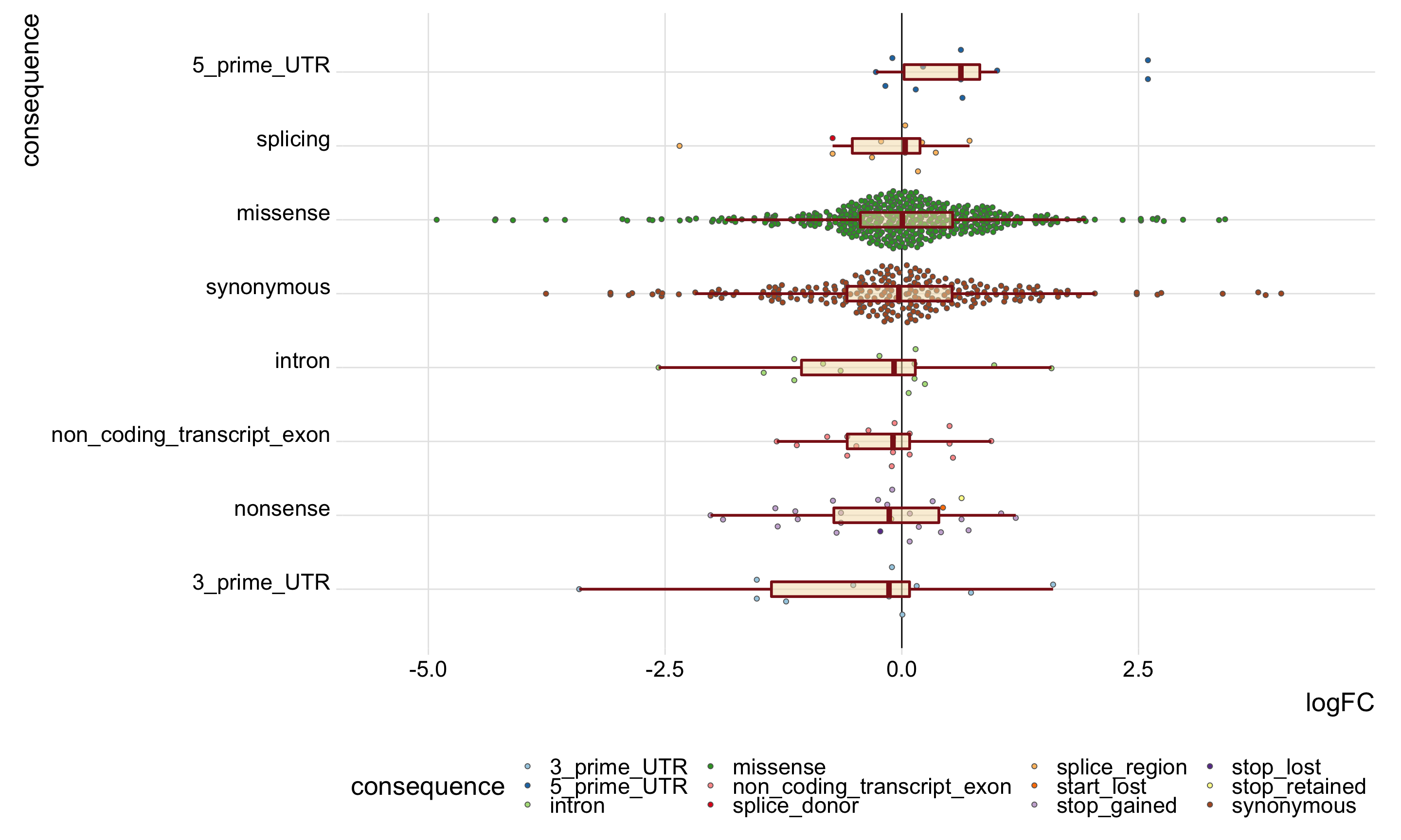
Expand here to see past versions of logfc-box-simple-1.png:
| Version | Author | Date |
|---|---|---|
| d2e8b31 | davismcc | 2018-08-19 |
ggsave("figures/mutated_genes/alllines_mutgenes_logfc-box_by_simple_vep_anno_allcells.png",
       height = 9, width = 15)
ggsave("figures/mutated_genes/alllines_mutgenes_logfc-box_by_simple_vep_anno_allcells.pdf",
       height = 9, width = 15)
ggsave("figures/mutated_genes/alllines_mutgenes_logfc-box_by_simple_vep_anno_allcells.svg",
       height = 9, width = 15)
On the evidence of the plot above it does not look like stricter filtering of variants fundmentally changes the results. It still does not look possible to discern differences in the logFC distributions of mutated genes between different annotation categories for variants.
DE for mutated clone: fitting PCs
We can also get DE results comparing mutated clone to all unmutated clones, fitting the first couple of PCs in the model to see if this accounts for unwanted variation and increases power to detect differences in expression between mutated and unwanted clones for mutated genes.
## run DE for mutated cells vs unmutated cells using existing DE results
## fitting PCs as covariates in DE model
mut_genes_df_allcells_list_PCreg <- list()
for (don in names(de_res[["sce_list_unst"]])) {
    cat("working on ", don, "\n")
    sites_tmp <- sites_by_line_gr[sites_by_line_gr$donor_short_id == don]
    ov_tmp <- findOverlaps(sce_de_list_gr[[don]], sites_tmp)
    sce_tmp <- de_res[["sce_list_unst"]][[don]][queryHits(ov_tmp),]
    sites_tmp <- sites_tmp[subjectHits(ov_tmp)]
    sites_tmp$gene <- rownames(sce_tmp)
    dge_tmp <- de_res[["dge_list"]][[don]]
    dge_tmp <- dge_tmp[intersect(rownames(dge_tmp), sites_tmp$gene),]
    base_design <- dge_tmp$design[, !grepl("assigned", colnames(dge_tmp$design))]
    de_tbl_tmp <- data.frame(line = don,
                             gene = sites_tmp$gene,
                             hgnc_symbol = gsub(".*_", "", sites_tmp$gene),
                             ensembl_gene_id = gsub("_.*", "", sites_tmp$gene),
                             var_id = sites_tmp$var_id,
                             location = sites_tmp$Location,
                             consequence = sites_tmp$Consequence,
                             clone_presence = sites_tmp$clone_presence,
                             logFC = NA, logCPM = NA, F = NA, PValue = NA,
                             comment = "", stringsAsFactors = FALSE)
    pca_tmp <- reducedDim(runPCA(
        de_res[["sce_list_unst"]][[don]], ntop = 500, ncomponents = 5), "PCA")
    for (i in seq_len(length(sites_tmp))) {
        clones_tmp <- strsplit(sites_tmp$clone_presence[i], split = "&")[[1]]
        mutatedclone <- as.numeric(sce_tmp$assigned %in% clones_tmp)
        dsgn_tmp <- cbind(base_design, pca_tmp[, 1], data.frame(mutatedclone))
        if (sites_tmp$gene[i] %in% rownames(dge_tmp) && is.fullrank(dsgn_tmp)) {
            qlfit_tmp <- glmQLFit(dge_tmp[sites_tmp$gene[i],], dsgn_tmp)
            de_tmp <- glmQLFTest(qlfit_tmp, coef = ncol(dsgn_tmp))
            de_tbl_tmp$logFC[i] <- de_tmp$table$logFC
            de_tbl_tmp$logCPM[i] <- de_tmp$table$logCPM
            de_tbl_tmp$F[i] <- de_tmp$table$F
            de_tbl_tmp$PValue[i] <- de_tmp$table$PValue
        }
        if (!(sites_tmp$gene[i] %in% rownames(dge_tmp)))
            de_tbl_tmp$comment[i] <- "gene did not pass DE filters"
        if (!is.fullrank(dsgn_tmp))
            de_tbl_tmp$comment[i] <- "insufficient cells assigned to clone"
    }
    mut_genes_df_allcells_list_PCreg[[don]] <- de_tbl_tmp
}
working on euts
working on fawm
working on feec
working on fikt
working on garx
working on gesg
working on heja
working on hipn
working on ieki
working on joxm
working on kuco
working on laey
working on lexy
working on naju
working on nusw
working on oaaz
working on oilg
working on pipw
working on puie
working on qayj
working on qolg
working on qonc
working on rozh
working on sehl
working on ualf
working on vass
working on vuna
working on wahn
working on wetu
working on xugn
working on zoxy mut_genes_df_allcells_PCreg <- do.call("bind_rows", mut_genes_df_allcells_list_PCreg)
## add FDRs for genes tested here for DE
ihw_res_all <- ihw(PValue ~ logCPM, data = mut_genes_df_allcells_PCreg, alpha = 0.2)
mut_genes_df_allcells_PCreg$FDR <- adj_pvalues(ihw_res_all)
## add simplified consequence categories
mut_genes_df_allcells_PCreg$consequence_simplified <-
mut_genes_df_allcells_PCreg$consequence
mut_genes_df_allcells_PCreg$consequence_simplified[
mut_genes_df_allcells_PCreg$consequence_simplified %in%
c("stop_retained", "start_lost", "stop_lost", "stop_gained")] <- "nonsense"
mut_genes_df_allcells_PCreg$consequence_simplified[
mut_genes_df_allcells_PCreg$consequence_simplified %in%
c("splice_donor", "splice_acceptor", "splice_region")] <- "splicing"
table(mut_genes_df_allcells_PCreg$consequence_simplified)
               3_prime_UTR                5_prime_UTR
                        27                         12
                    intron                   missense
                        20                        650
non_coding_transcript_exon                   nonsense
                        20                         39
                  splicing                 synonymous
21 351 dplyr::arrange(mut_genes_df_allcells_PCreg, FDR) %>%
dplyr::select(-location) %>%
DT::datatable(., options = list(pageLength = 20))data_frame(PValue_default = mut_genes_df_allcells[["PValue"]],
PValue_PCreg = mut_genes_df_allcells_PCreg[["PValue"]],
sig_default = mut_genes_df_allcells[["FDR"]] < 0.1,
sig_PCreg = mut_genes_df_allcells_PCreg[["FDR"]] < 0.1) %>%
ggplot(aes(x = -log10(PValue_default), y = -log10(PValue_PCreg),
shape = sig_default, colour = sig_PCreg)) +
geom_point() +
geom_smooth(aes(group = 1), colour = "firebrick") +
geom_abline(slope = 1, intercept = 0) +
scale_color_manual(values = c("gray60", "black"))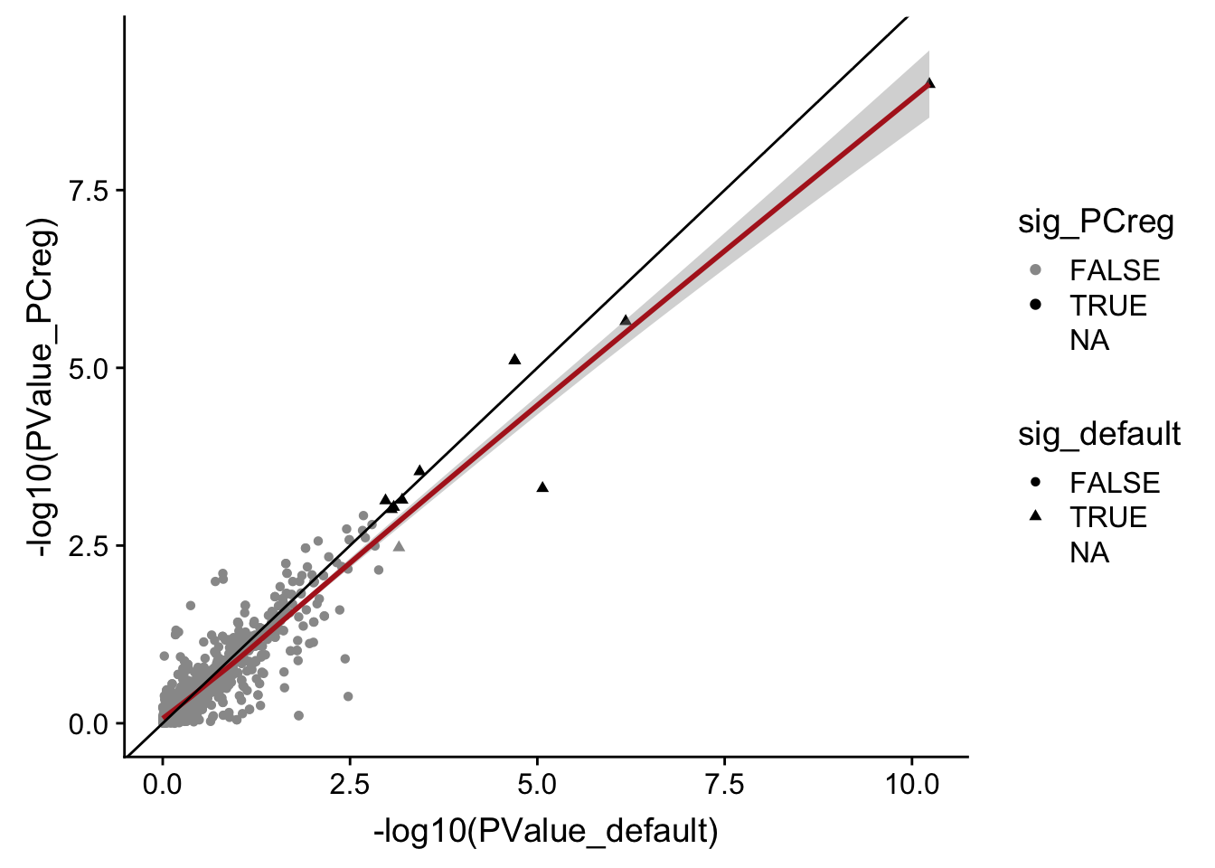
Expand here to see past versions of mut-genes-fit-pcs-2.png:
| Version | Author | Date |
|---|---|---|
| d2e8b31 | davismcc | 2018-08-19 |
There is thus very little change in DE results when regressing out 5 PCs in these DE models.
DE for mutated clones: fitting cell cycle scores
We can also check to see if accounting for cell cycle scores in the DE model increases power to detect differential expression between mutated and unmutated clones for mutated genes.
## run DE for mutated cells vs unmutated cells using existing DE results
## fitting PCs as covariates in DE model
mut_genes_df_allcells_list_CCreg <- list()
for (don in names(de_res[["sce_list_unst"]])) {
    cat("working on ", don, "\n")
    sites_tmp <- sites_by_line_gr[sites_by_line_gr$donor_short_id == don]
    ov_tmp <- findOverlaps(sce_de_list_gr[[don]], sites_tmp)
    sce_tmp <- de_res[["sce_list_unst"]][[don]][queryHits(ov_tmp),]
    sites_tmp <- sites_tmp[subjectHits(ov_tmp)]
    sites_tmp$gene <- rownames(sce_tmp)
    dge_tmp <- de_res[["dge_list"]][[don]]
    dge_tmp <- dge_tmp[intersect(rownames(dge_tmp), sites_tmp$gene),]
    base_design <- dge_tmp$design[, !grepl("assigned", colnames(dge_tmp$design))]
    de_tbl_tmp <- data.frame(line = don,
                             gene = sites_tmp$gene,
                             hgnc_symbol = gsub(".*_", "", sites_tmp$gene),
                             ensembl_gene_id = gsub("_.*", "", sites_tmp$gene),
                             var_id = sites_tmp$var_id,
                             location = sites_tmp$Location,
                             consequence = sites_tmp$Consequence,
                             clone_presence = sites_tmp$clone_presence,
                             logFC = NA, logCPM = NA, F = NA, PValue = NA,
                             comment = "", stringsAsFactors = FALSE)
    G1 <- de_res[["sce_list_unst"]][[don]]$G1
    S <- de_res[["sce_list_unst"]][[don]]$S
    G2M <- de_res[["sce_list_unst"]][[don]]$G2M
    for (i in seq_len(length(sites_tmp))) {
        clones_tmp <- strsplit(sites_tmp$clone_presence[i], split = "&")[[1]]
        mutatedclone <- as.numeric(sce_tmp$assigned %in% clones_tmp)
        dsgn_tmp <- cbind(base_design, G1, S, G2M, data.frame(mutatedclone))
        if (sites_tmp$gene[i] %in% rownames(dge_tmp) && is.fullrank(dsgn_tmp)) {
            qlfit_tmp <- glmQLFit(dge_tmp[sites_tmp$gene[i],], dsgn_tmp)
            de_tmp <- glmQLFTest(qlfit_tmp, coef = ncol(dsgn_tmp))
            de_tbl_tmp$logFC[i] <- de_tmp$table$logFC
            de_tbl_tmp$logCPM[i] <- de_tmp$table$logCPM
            de_tbl_tmp$F[i] <- de_tmp$table$F
            de_tbl_tmp$PValue[i] <- de_tmp$table$PValue
        }
        if (!(sites_tmp$gene[i] %in% rownames(dge_tmp)))
            de_tbl_tmp$comment[i] <- "gene did not pass DE filters"
        if (!is.fullrank(dsgn_tmp))
            de_tbl_tmp$comment[i] <- "insufficient cells assigned to clone"
    }
    mut_genes_df_allcells_list_CCreg[[don]] <- de_tbl_tmp
}
working on euts
working on fawm
working on feec
working on fikt
working on garx
working on gesg
working on heja
working on hipn
working on ieki
working on joxm
working on kuco
working on laey
working on lexy
working on naju
working on nusw
working on oaaz
working on oilg
working on pipw
working on puie
working on qayj
working on qolg
working on qonc
working on rozh
working on sehl
working on ualf
working on vass
working on vuna
working on wahn
working on wetu
working on xugn
working on zoxy mut_genes_df_allcells_CCreg <- do.call("bind_rows", mut_genes_df_allcells_list_CCreg)
## add FDRs for genes tested here for DE
ihw_res_all <- ihw(PValue ~ logCPM, data = mut_genes_df_allcells_CCreg, alpha = 0.2)
mut_genes_df_allcells_CCreg$FDR <- adj_pvalues(ihw_res_all)
## add simplified consequence categories
mut_genes_df_allcells_CCreg$consequence_simplified <-
mut_genes_df_allcells_CCreg$consequence
mut_genes_df_allcells_CCreg$consequence_simplified[
mut_genes_df_allcells_CCreg$consequence_simplified %in%
c("stop_retained", "start_lost", "stop_lost", "stop_gained")] <- "nonsense"
mut_genes_df_allcells_CCreg$consequence_simplified[
mut_genes_df_allcells_CCreg$consequence_simplified %in%
c("splice_donor", "splice_acceptor", "splice_region")] <- "splicing"
dplyr::arrange(mut_genes_df_allcells_CCreg, FDR) %>%
dplyr::select(-location) %>%
DT::datatable(., options = list(pageLength = 20))data_frame(PValue_default = mut_genes_df_allcells[["PValue"]],
PValue_CCreg = mut_genes_df_allcells_CCreg[["PValue"]],
sig_default = mut_genes_df_allcells[["FDR"]] < 0.1,
sig_PCreg = mut_genes_df_allcells_CCreg[["FDR"]] < 0.1) %>%
ggplot(aes(x = -log10(PValue_default), y = -log10(PValue_CCreg),
shape = sig_default, colour = sig_PCreg)) +
geom_point() +
geom_smooth(aes(group = 1), colour = "firebrick") +
geom_abline(slope = 1, intercept = 0) +
scale_color_manual(values = c("gray60", "black"))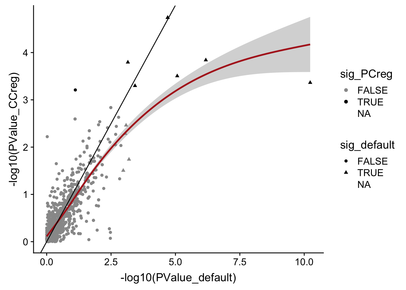
Expand here to see past versions of mut-genes-fit-cc-2.png:
| Version | Author | Date |
|---|---|---|
| d2e8b31 | davismcc | 2018-08-19 |
Accounting for cell cycle scores (inferred with cyclone) in the DE model does not drastically change DE results, but perhaps does reduce power to find differences in expression between mutated and unmutated clones.
Characterising mutations and mutated genes
First, we can look at the number of variants annotated to the different VEP categories and assigned to combinations of clones, aggregated across all lines.
sites_by_line %>% group_by(Consequence, clone_presence) %>%
    summarise(n_vars = n()) %>%
ggplot(aes(x = n_vars, y = reorder(Consequence, n_vars, max),
       colour = reorder(Consequence, n_vars, max))) +
    geom_point(size = 5) +
    geom_segment(aes(x = 0, y = Consequence, xend = n_vars, yend = Consequence)) +
    facet_wrap(~clone_presence) +
    scale_color_manual(values = colorRampPalette(brewer.pal(8, "Accent"))(18)) +
    guides(colour = FALSE) +
    ggtitle("Clone tagging variants by consequence class: all lines") +
    xlab("number of variants") + ylab("consequence") +
    theme_bw(16)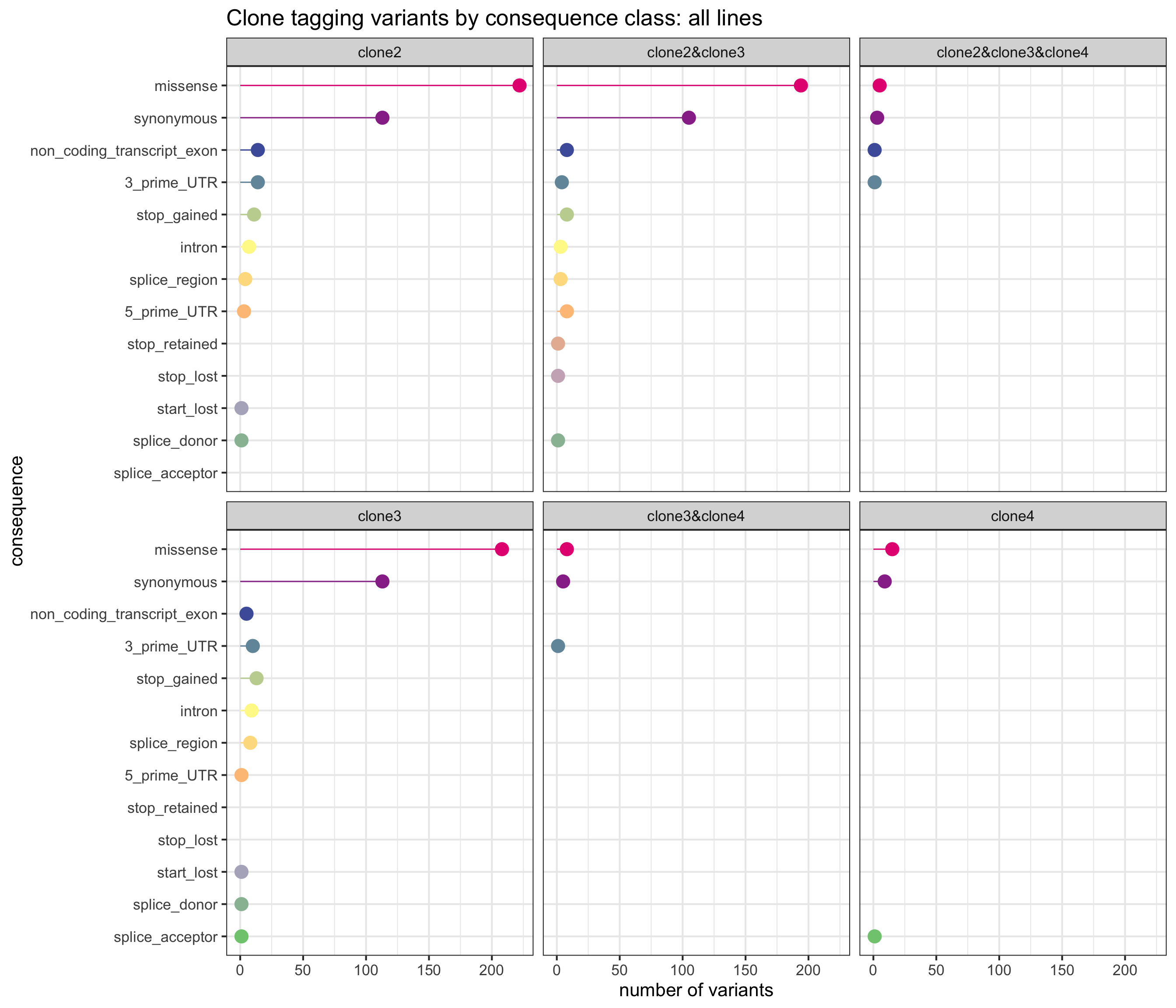
Expand here to see past versions of unnamed-chunk-12-1.png:
| Version | Author | Date |
|---|---|---|
| d2e8b31 | davismcc | 2018-08-19 |
We can also produce a similar plot, but showing the total number variants in each annotation category for each line separately.
sites_by_line %>% group_by(Consequence, donor_short_id) %>%
    summarise(n_vars = n()) %>%
ggplot(aes(x = n_vars, y = reorder(Consequence, n_vars, max),
       colour = reorder(Consequence, n_vars, max))) +
    geom_point(size = 5) +
    geom_segment(aes(x = 0, y = Consequence, xend = n_vars, yend = Consequence)) +
    facet_wrap(~donor_short_id) +
#    scale_color_brewer(palette = "Set2") +
    scale_color_manual(values = colorRampPalette(brewer.pal(8, "Accent"))(18)) +
    guides(colour = FALSE) +
    ggtitle("Clone tagging variants by consequence class: all lines") +
    xlab("number of variants") + ylab("consequence") +
    theme_bw(16)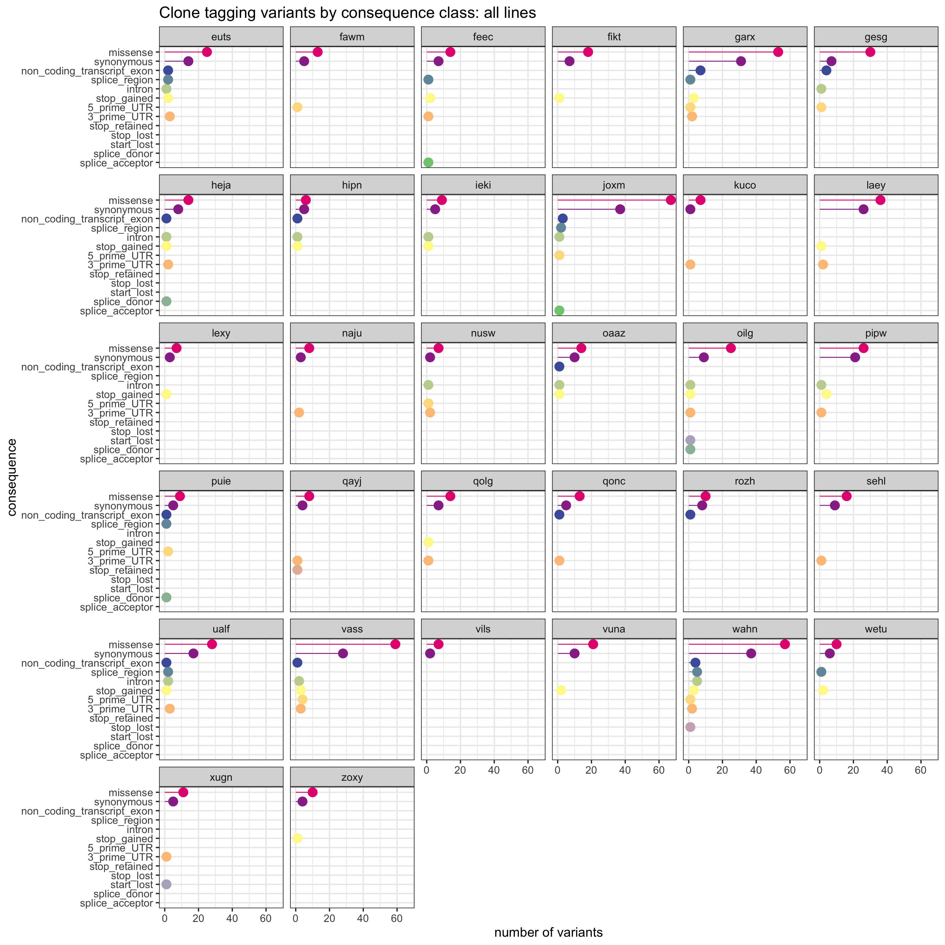
Expand here to see past versions of unnamed-chunk-13-1.png:
| Version | Author | Date |
|---|---|---|
| d2e8b31 | davismcc | 2018-08-19 |
Genes with more than one mutation
It’s also of interest to know if there are genes with multiple mutations in a line.
df_genes_multi_vars <- mut_genes_df_allcells %>%
  dplyr::mutate(pos = as.numeric(gsub("chr.+:([0-9]+)_.*", "\\1", var_id))) %>%
  group_by(line, hgnc_symbol) %>%
  summarise(n_variants_in_gene = n(),
            max_dist_btw_vars = range(pos)[2] - range(pos)[1])
df_genes_multi_vars %>%
  dplyr::filter(n_variants_in_gene > 1.5, max_dist_btw_vars > 1.5)
# A tibble: 4 x 4
# Groups: line [2]
line hgnc_symbol n_variants_in_gene max_dist_btw_vars
<chr> <chr> <int> <dbl>
1 joxm COL1A1 2 1815
2 joxm TBC1D9B 3 29054
3 qonc MAPK12 3 27
4 qonc WIPI2 2 1187There are only 4 genes, across all lines, that have more than one (non-dinucleotide) somatic variant.
idx <- (df_genes_multi_vars$n_variants_in_gene > 1.5 &
          df_genes_multi_vars$max_dist_btw_vars > 1.5)
mut_genes_df_allcells %>%
  dplyr::filter(line %in% df_genes_multi_vars[["line"]][idx],
               hgnc_symbol %in% df_genes_multi_vars[["hgnc_symbol"]][idx]) %>%
  DT::datatable()
In the case of the COL1A1 gene in joxm, there are two splicing variants (one a splice-acceptor variant and one a more general splice-region variant), and cells in the mutated clones have significantly lower expression than the unmutated clones for this gene. For the remaining genes with more than one somatic variant, there is no significant difference in gene expression between the mutated and unmutated clones.
Mutations in cell cycle genes
Given the results of the transcriptome-wide differential expression analyses, it would be interesting to know if cell cycle genes specifically harbour mutations. To explore this, we first obtain the set of genes belonging to cell cycle gene sets in the MSigDB c2 gene set collection.
load(file.path("data/human_c2_v5p2.rdata"))

cellcycle_entrezid <- Hs.c2[grep("CELL_CYCL", names(Hs.c2))] %>%
  unlist %>% unique
mapped_genes <- mappedkeys(org.Hs.egSYMBOL)
cellcycle_entrezid <- cellcycle_entrezid[cellcycle_entrezid %in% mapped_genes]
xx <- unlist(as.list(org.Hs.egSYMBOL[cellcycle_entrezid]))
xx <- sort(unique(xx))
This yields a list of 1243 genes annotated to be relevant to the cell cycle.
Let us look at the number of variants used for clonal reconstruction (a strictly filtered set) across VEP annotation categories that lie in cell cycle genes.
df_cc_vars <- mut_genes_df_allcells %>%
  dplyr::filter(hgnc_symbol %in% xx) %>%
  group_by(line, consequence_simplified) %>%
  summarise(n_vars = n())
df_cc_vars <- left_join(
  expand.grid(line = levels(as.factor(mut_genes_df_allcells$line)),
              consequence_simplified = levels(as.factor(
                mut_genes_df_allcells$consequence_simplified))),
  df_cc_vars)
df_cc_vars[is.na(df_cc_vars)] <- 0

ggplot(df_cc_vars,
       aes(x = n_vars, y = reorder(consequence_simplified, n_vars, max),
           colour = reorder(consequence_simplified, n_vars, max),
           fill = reorder(consequence_simplified, n_vars, max))) +
  geom_segment(aes(x = 0, y = consequence_simplified, xend = n_vars,
                   yend = consequence_simplified)) +
  geom_point(size = 5, colour = "gray50", shape = 21) +
  facet_wrap(~line, ncol = 4) +
  scale_color_manual(values = colorRampPalette(brewer.pal(8, "Accent"))(18)) +
  scale_fill_manual(values = colorRampPalette(brewer.pal(8, "Accent"))(18)) +
  guides(colour = FALSE, fill = FALSE) +
  ggtitle("Variants in proliferation genes: all lines") +
  xlab("number of variants") + ylab("consequence") +
  theme_bw(16)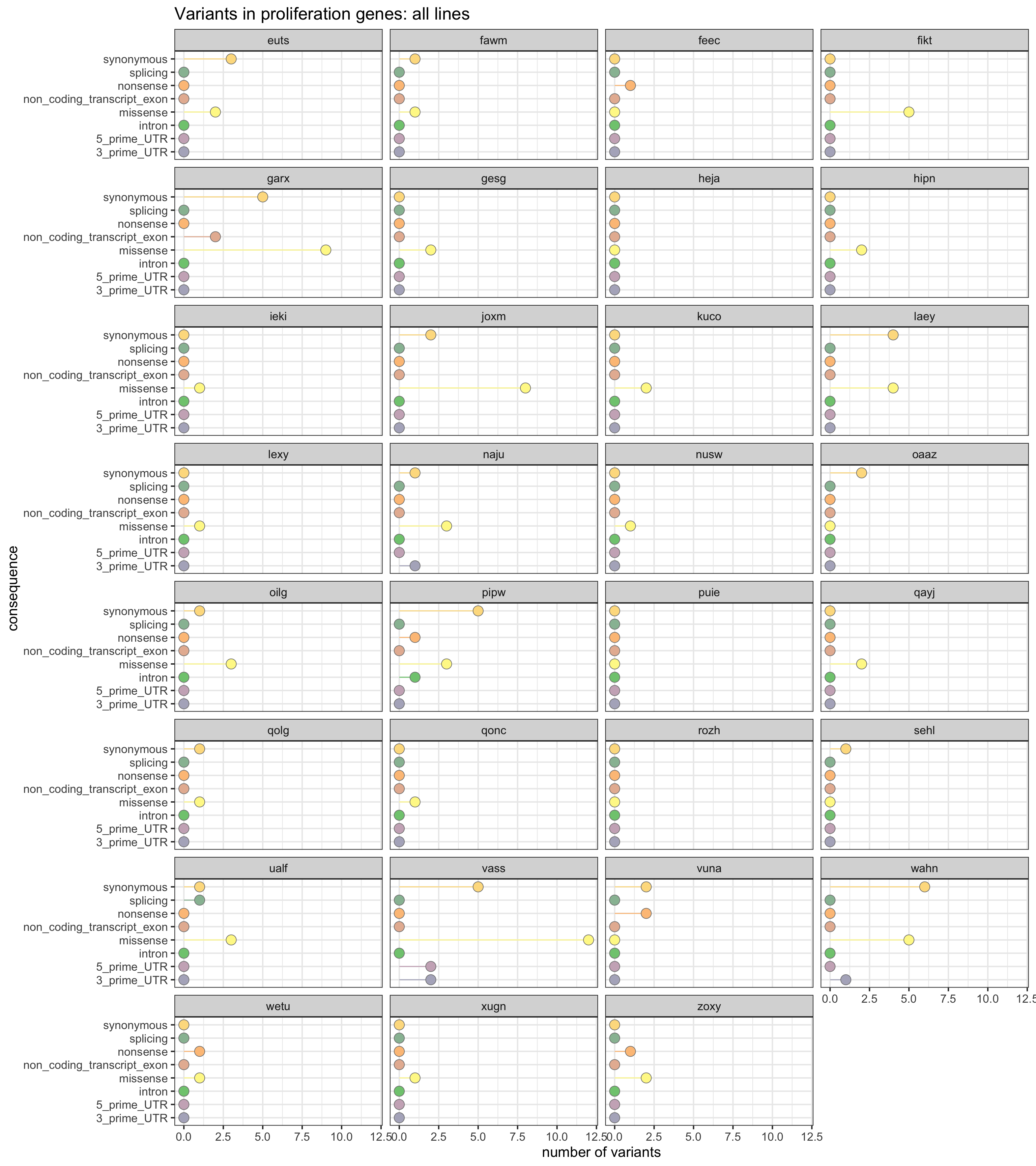
Mutations in proliferation genes
We can also look at the load of mutations in genes annotated to MSigDB c2 proliferation gene sets.
prolif_entrezid <- Hs.c2[grep("PROLIF", names(Hs.c2))] %>%
  unlist %>% unique
prolif_entrezid <- prolif_entrezid[prolif_entrezid %in% mapped_genes]
x2 <- unlist(as.list(org.Hs.egSYMBOL[prolif_entrezid]))
x2 <- sort(unique(x2))
This yields a list of 1219 genes annotated to be relevant to the cell cycle.
df_prolif_vars <- mut_genes_df_allcells %>%
  dplyr::filter(hgnc_symbol %in% x2) %>%
  group_by(line, consequence_simplified) %>%
  summarise(n_vars = n())
df_prolif_vars <- left_join(
  expand.grid(line = levels(as.factor(mut_genes_df_allcells$line)),
              consequence_simplified = levels(as.factor(
                mut_genes_df_allcells$consequence_simplified))),
  df_prolif_vars)
df_prolif_vars[is.na(df_prolif_vars)] <- 0

ggplot(df_prolif_vars,
       aes(x = n_vars, y = reorder(consequence_simplified, n_vars, max),
           colour = reorder(consequence_simplified, n_vars, max),
           fill = reorder(consequence_simplified, n_vars, max))) +
  geom_segment(aes(x = 0, y = consequence_simplified, xend = n_vars,
                   yend = consequence_simplified)) +
  geom_point(size = 5, colour = "gray50", shape = 21) +
  facet_wrap(~line, ncol = 4) +
  scale_color_manual(values = colorRampPalette(brewer.pal(8, "Accent"))(18)) +
  scale_fill_manual(values = colorRampPalette(brewer.pal(8, "Accent"))(18)) +
  guides(colour = FALSE, fill = FALSE) +
  ggtitle("Variants in cell cycle genes: all lines") +
  xlab("number of variants") + ylab("consequence") +
  theme_bw(16)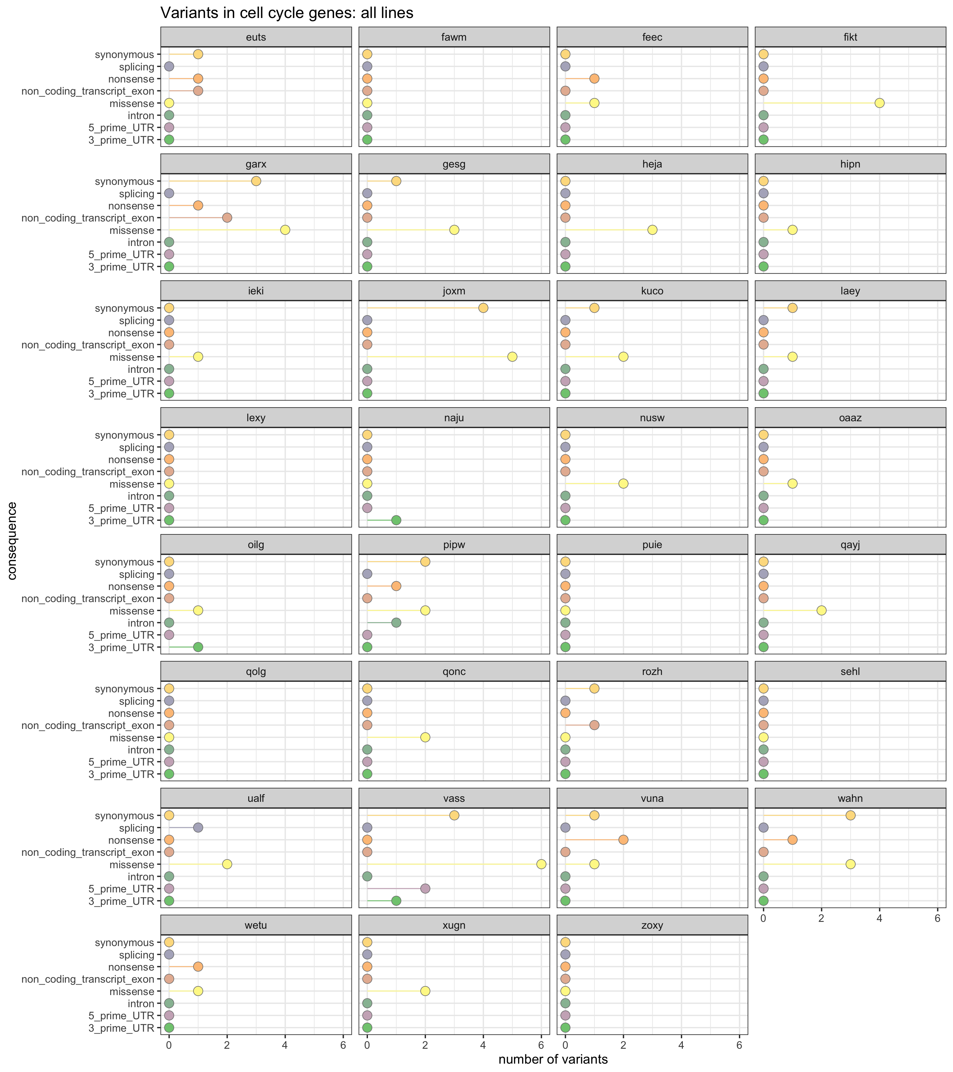
Finally, create a data.frame that contains the counts of variants annotated to different classes of genes and VEP classes, and save to file for use in other analyses.
colnames(df_cc_vars) <- c("line", "consequence", "n_vars_cellcycle_genes")
colnames(df_prolif_vars) <- c("line", "consequence", "n_vars_proliferation_genes")
df_all_vars <- mut_genes_df_allcells %>%
  group_by(line, consequence_simplified) %>%
  summarise(n_vars_all_genes = n())
df_all_vars <- left_join(
  expand.grid(line = levels(as.factor(mut_genes_df_allcells$line)),
              consequence_simplified = levels(as.factor(
                mut_genes_df_allcells$consequence_simplified))),
  df_all_vars)
df_all_vars[is.na(df_all_vars)] <- 0
colnames(df_all_vars) <- c("line", "consequence", "n_vars_all_genes")

df_nvars <- inner_join(inner_join(df_all_vars, df_cc_vars), df_prolif_vars) %>%
  as_data_frame

readr::write_tsv(df_nvars, "output/nvars_by_category_by_line.tsv")

df_nvars %>%
  DT::datatable(., options = list(pageLength = 20))
We can also look at the total mutational load for each of the lines.
df_nvars %>%
  group_by(line) %>%
  summarise(nvars = sum(n_vars_all_genes)) %>% print(n = Inf)
# A tibble: 31 x 2
line nvars
<chr> <dbl>
1 euts 49
2 fawm 20
3 feec 24
4 fikt 27
5 garx 95
6 gesg 45
7 heja 32
8 hipn 11
9 ieki 15
10 joxm 116
11 kuco 9
12 laey 63
13 lexy 11
14 naju 15
15 nusw 13
16 oaaz 24
17 oilg 38
18 pipw 56
19 puie 18
20 qayj 16
21 qolg 28
22 qonc 20
23 rozh 16
24 sehl 29
25 ualf 48
26 vass 101
27 vuna 35
28 wahn 115
29 wetu 19
30 xugn 18
31 zoxy 14Conclusions
We find a small number of somatic variants to associate with differential expression between mutated and unmutated cells/clones. Unfortunately, in this set of variants and lines (with relatively small sample size in terms of numbers of cells), we cannot make any claims about different effects on expression of somatic variants with different functional annotations.
Session information
devtools::session_info() setting value
version R version 3.5.1 (2018-07-02)
system x86_64, darwin15.6.0
ui X11
language (EN)
collate en_GB.UTF-8
tz Europe/London
date 2018-08-25
package * version date source
AnnotationDbi * 1.42.1 2018-05-08 Bioconductor
assertthat 0.2.0 2017-04-11 CRAN (R 3.5.0)
backports 1.1.2 2017-12-13 CRAN (R 3.5.0)
base * 3.5.1 2018-07-05 local
beeswarm 0.2.3 2016-04-25 CRAN (R 3.5.0)
bindr 0.1.1 2018-03-13 CRAN (R 3.5.0)
bindrcpp * 0.2.2 2018-03-29 CRAN (R 3.5.0)
Biobase * 2.40.0 2018-05-01 Bioconductor
BiocGenerics * 0.26.0 2018-05-01 Bioconductor
BiocParallel * 1.14.2 2018-07-08 Bioconductor
bit 1.1-14 2018-05-29 CRAN (R 3.5.0)
bit64 0.9-7 2017-05-08 CRAN (R 3.5.0)
bitops 1.0-6 2013-08-17 CRAN (R 3.5.0)
blob 1.1.1 2018-03-25 CRAN (R 3.5.0)
broom 0.5.0 2018-07-17 CRAN (R 3.5.0)
cellranger 1.1.0 2016-07-27 CRAN (R 3.5.0)
cli 1.0.0 2017-11-05 CRAN (R 3.5.0)
colorspace 1.3-2 2016-12-14 CRAN (R 3.5.0)
compiler 3.5.1 2018-07-05 local
cowplot * 0.9.3 2018-07-15 CRAN (R 3.5.0)
crayon 1.3.4 2017-09-16 CRAN (R 3.5.0)
crosstalk 1.0.0 2016-12-21 CRAN (R 3.5.0)
data.table 1.11.4 2018-05-27 CRAN (R 3.5.0)
datasets * 3.5.1 2018-07-05 local
DBI 1.0.0 2018-05-02 CRAN (R 3.5.0)
DelayedArray * 0.6.5 2018-08-15 Bioconductor
DelayedMatrixStats 1.2.0 2018-05-01 Bioconductor
devtools 1.13.6 2018-06-27 CRAN (R 3.5.0)
digest 0.6.16 2018-08-22 CRAN (R 3.5.0)
dplyr * 0.7.6 2018-06-29 CRAN (R 3.5.1)
DT 0.4 2018-01-30 CRAN (R 3.5.0)
edgeR * 3.22.3 2018-06-21 Bioconductor
evaluate 0.11 2018-07-17 CRAN (R 3.5.0)
fansi 0.3.0 2018-08-13 CRAN (R 3.5.0)
fdrtool 1.2.15 2015-07-08 CRAN (R 3.5.0)
forcats * 0.3.0 2018-02-19 CRAN (R 3.5.0)
gdtools * 0.1.7 2018-02-27 CRAN (R 3.5.0)
GenomeInfoDb * 1.16.0 2018-05-01 Bioconductor
GenomeInfoDbData 1.1.0 2018-04-25 Bioconductor
GenomicRanges * 1.32.6 2018-07-20 Bioconductor
ggbeeswarm 0.6.0 2017-08-07 CRAN (R 3.5.0)
ggExtra 0.8 2018-04-04 CRAN (R 3.5.0)
ggforce * 0.1.3 2018-07-07 CRAN (R 3.5.0)
ggplot2 * 3.0.0 2018-07-03 CRAN (R 3.5.0)
ggrepel * 0.8.0 2018-05-09 CRAN (R 3.5.0)
ggridges * 0.5.0 2018-04-05 CRAN (R 3.5.0)
git2r 0.23.0 2018-07-17 CRAN (R 3.5.0)
glue 1.3.0 2018-07-17 CRAN (R 3.5.0)
graphics * 3.5.1 2018-07-05 local
grDevices * 3.5.1 2018-07-05 local
grid 3.5.1 2018-07-05 local
gridExtra 2.3 2017-09-09 CRAN (R 3.5.0)
gtable 0.2.0 2016-02-26 CRAN (R 3.5.0)
haven 1.1.2 2018-06-27 CRAN (R 3.5.0)
hms 0.4.2 2018-03-10 CRAN (R 3.5.0)
htmltools 0.3.6 2017-04-28 CRAN (R 3.5.0)
htmlwidgets 1.2 2018-04-19 CRAN (R 3.5.0)
httpuv 1.4.5 2018-07-19 CRAN (R 3.5.0)
httr 1.3.1 2017-08-20 CRAN (R 3.5.0)
IHW * 1.8.0 2018-05-01 Bioconductor
IRanges * 2.14.11 2018-08-24 Bioconductor
jsonlite 1.5 2017-06-01 CRAN (R 3.5.0)
knitr 1.20 2018-02-20 CRAN (R 3.5.0)
labeling 0.3 2014-08-23 CRAN (R 3.5.0)
later 0.7.3 2018-06-08 CRAN (R 3.5.0)
lattice 0.20-35 2017-03-25 CRAN (R 3.5.1)
lazyeval 0.2.1 2017-10-29 CRAN (R 3.5.0)
limma * 3.36.2 2018-06-21 Bioconductor
locfit 1.5-9.1 2013-04-20 CRAN (R 3.5.0)
lpsymphony 1.8.0 2018-05-01 Bioconductor (R 3.5.0)
lubridate 1.7.4 2018-04-11 CRAN (R 3.5.0)
magrittr 1.5 2014-11-22 CRAN (R 3.5.0)
MASS 7.3-50 2018-04-30 CRAN (R 3.5.1)
Matrix 1.2-14 2018-04-13 CRAN (R 3.5.1)
matrixStats * 0.54.0 2018-07-23 CRAN (R 3.5.0)
memoise 1.1.0 2017-04-21 CRAN (R 3.5.0)
methods * 3.5.1 2018-07-05 local
mgcv 1.8-24 2018-06-23 CRAN (R 3.5.1)
mime 0.5 2016-07-07 CRAN (R 3.5.0)
miniUI 0.1.1.1 2018-05-18 CRAN (R 3.5.0)
modelr 0.1.2 2018-05-11 CRAN (R 3.5.0)
munsell 0.5.0 2018-06-12 CRAN (R 3.5.0)
nlme 3.1-137 2018-04-07 CRAN (R 3.5.1)
org.Hs.eg.db * 3.6.0 2018-05-15 Bioconductor
parallel * 3.5.1 2018-07-05 local
pillar 1.3.0 2018-07-14 CRAN (R 3.5.0)
pkgconfig 2.0.2 2018-08-16 CRAN (R 3.5.0)
plyr 1.8.4 2016-06-08 CRAN (R 3.5.0)
promises 1.0.1 2018-04-13 CRAN (R 3.5.0)
purrr * 0.2.5 2018-05-29 CRAN (R 3.5.0)
R.methodsS3 1.7.1 2016-02-16 CRAN (R 3.5.0)
R.oo 1.22.0 2018-04-22 CRAN (R 3.5.0)
R.utils 2.6.0 2017-11-05 CRAN (R 3.5.0)
R6 2.2.2 2017-06-17 CRAN (R 3.5.0)
RColorBrewer * 1.1-2 2014-12-07 CRAN (R 3.5.0)
Rcpp 0.12.18 2018-07-23 CRAN (R 3.5.0)
RCurl 1.95-4.11 2018-07-15 CRAN (R 3.5.0)
readr * 1.1.1 2017-05-16 CRAN (R 3.5.0)
readxl 1.1.0 2018-04-20 CRAN (R 3.5.0)
reshape2 1.4.3 2017-12-11 CRAN (R 3.5.0)
rhdf5 2.24.0 2018-05-01 Bioconductor
Rhdf5lib 1.2.1 2018-05-17 Bioconductor
rjson 0.2.20 2018-06-08 CRAN (R 3.5.0)
rlang * 0.2.2 2018-08-16 CRAN (R 3.5.0)
rmarkdown 1.10 2018-06-11 CRAN (R 3.5.0)
rprojroot 1.3-2 2018-01-03 CRAN (R 3.5.0)
RSQLite 2.1.1 2018-05-06 CRAN (R 3.5.0)
rstudioapi 0.7 2017-09-07 CRAN (R 3.5.0)
rvest 0.3.2 2016-06-17 CRAN (R 3.5.0)
S4Vectors * 0.18.3 2018-06-08 Bioconductor
scales 1.0.0 2018-08-09 CRAN (R 3.5.0)
scater * 1.9.12 2018-08-03 Bioconductor
shiny 1.1.0 2018-05-17 CRAN (R 3.5.0)
SingleCellExperiment * 1.2.0 2018-05-01 Bioconductor
slam 0.1-43 2018-04-23 CRAN (R 3.5.0)
stats * 3.5.1 2018-07-05 local
stats4 * 3.5.1 2018-07-05 local
stringi 1.2.4 2018-07-20 CRAN (R 3.5.0)
stringr * 1.3.1 2018-05-10 CRAN (R 3.5.0)
SummarizedExperiment * 1.10.1 2018-05-11 Bioconductor
superheat * 0.1.0 2017-02-04 CRAN (R 3.5.0)
svglite 1.2.1 2017-09-11 CRAN (R 3.5.0)
tibble * 1.4.2 2018-01-22 CRAN (R 3.5.0)
tidyr * 0.8.1 2018-05-18 CRAN (R 3.5.0)
tidyselect 0.2.4 2018-02-26 CRAN (R 3.5.0)
tidyverse * 1.2.1 2017-11-14 CRAN (R 3.5.0)
tools 3.5.1 2018-07-05 local
tweenr 0.1.5 2016-10-10 CRAN (R 3.5.0)
tximport 1.8.0 2018-05-01 Bioconductor
units 0.6-0 2018-06-09 CRAN (R 3.5.0)
utf8 1.1.4 2018-05-24 CRAN (R 3.5.0)
utils * 3.5.1 2018-07-05 local
vipor 0.4.5 2017-03-22 CRAN (R 3.5.0)
viridis * 0.5.1 2018-03-29 CRAN (R 3.5.0)
viridisLite * 0.3.0 2018-02-01 CRAN (R 3.5.0)
whisker 0.3-2 2013-04-28 CRAN (R 3.5.0)
withr 2.1.2 2018-03-15 CRAN (R 3.5.0)
workflowr 1.1.1 2018-07-06 CRAN (R 3.5.0)
xml2 1.2.0 2018-01-24 CRAN (R 3.5.0)
xtable 1.8-2 2016-02-05 CRAN (R 3.5.0)
XVector 0.20.0 2018-05-01 Bioconductor
yaml 2.2.0 2018-07-25 CRAN (R 3.5.1)
zlibbioc 1.26.0 2018-05-01 Bioconductor This reproducible R Markdown analysis was created with workflowr 1.1.1