Differential expression across all donors

Last updated: 2018-11-09

workflowr checks: (Click a bullet for more information)

✔ R Markdown file: up-to-date

Great! Since the R Markdown file has been committed to the Git repository, you know the exact version of the code that produced these results.
✔ Environment: empty

Great job! The global environment was empty. Objects defined in the global environment can affect the analysis in your R Markdown file in unknown ways. For reproduciblity it’s best to always run the code in an empty environment.
✔ Seed: set.seed(20180807)

The command set.seed(20180807) was run prior to running the code in the R Markdown file. Setting a seed ensures that any results that rely on randomness, e.g. subsampling or permutations, are reproducible.
✔ Session information: recorded

Great job! Recording the operating system, R version, and package versions is critical for reproducibility.

✔ Repository version: f98a31e

Great! You are using Git for version control. Tracking code development and connecting the code version to the results is critical for reproducibility. The version displayed above was the version of the Git repository at the time these results were generated.

Note that you need to be careful to ensure that all relevant files for the analysis have been committed to Git prior to generating the results (you can use wflow_publish or wflow_git_commit). workflowr only checks the R Markdown file, but you know if there are other scripts or data files that it depends on. Below is the status of the Git repository when the results were generated:


Ignored files:
    Ignored:    .DS_Store
    Ignored:    .Rhistory
    Ignored:    .Rproj.user/
    Ignored:    .vscode/
    Ignored:    code/.DS_Store
    Ignored:    data/raw/
    Ignored:    src/.DS_Store
    Ignored:    src/Rmd/.Rhistory

Untracked files:
    Untracked:  Snakefile_clonality
    Untracked:  Snakefile_somatic_calling
    Untracked:  code/analysis_for_garx.Rmd
    Untracked:  code/selection/
    Untracked:  code/yuanhua/
    Untracked:  data/canopy/
    Untracked:  data/cell_assignment/
    Untracked:  data/de_analysis_FTv62/
    Untracked:  data/donor_info_070818.txt
    Untracked:  data/donor_info_core.csv
    Untracked:  data/donor_neutrality.tsv
    Untracked:  data/exome-point-mutations/
    Untracked:  data/fdr10.annot.txt.gz
    Untracked:  data/human_H_v5p2.rdata
    Untracked:  data/human_c2_v5p2.rdata
    Untracked:  data/human_c6_v5p2.rdata
    Untracked:  data/neg-bin-rsquared-petr.csv
    Untracked:  data/neutralitytestr-petr.tsv
    Untracked:  data/sce_merged_donors_cardelino_donorid_all_qc_filt.rds
    Untracked:  data/sce_merged_donors_cardelino_donorid_all_with_qc_labels.rds
    Untracked:  data/sce_merged_donors_cardelino_donorid_unstim_qc_filt.rds
    Untracked:  data/sces/
    Untracked:  data/selection/
    Untracked:  data/simulations/
    Untracked:  data/variance_components/
    Untracked:  figures/
    Untracked:  output/differential_expression/
    Untracked:  output/donor_specific/
    Untracked:  output/line_info.tsv
    Untracked:  output/nvars_by_category_by_donor.tsv
    Untracked:  output/nvars_by_category_by_line.tsv
    Untracked:  output/variance_components/
    Untracked:  references/
    Untracked:  tree.txt

Note that any generated files, e.g. HTML, png, CSS, etc., are not included in this status report because it is ok for generated content to have uncommitted changes.

Expand here to see past versions:

File	Version	Author	Date	Message
html	0540cdb	davismcc	2018-09-02	Build site.
html	f0ed980	davismcc	2018-08-31	Build site.
Rmd	1310c93	davismcc	2018-08-30	Tweaking plots
Rmd	acc5756	davismcc	2018-08-30	Latest tweaks.
Rmd	846dec4	davismcc	2018-08-30	Some small tweaks/additions to analyses
html	ca3438f	davismcc	2018-08-29	Build site.
Rmd	128fea5	davismcc	2018-08-29	Small bug fix
Rmd	dc78a95	davismcc	2018-08-29	Minor updates to analyses.
html	a056169	davismcc	2018-08-27	Addign updated docs
Rmd	c882c59	davismcc	2018-08-27	Fixing some typos
Rmd	8f74680	davismcc	2018-08-27	Adding a couple of extra plots
html	e573f2f	davismcc	2018-08-27	Build site.
html	9ec2a59	davismcc	2018-08-26	Build site.
html	36acf15	davismcc	2018-08-25	Build site.
Rmd	d618fe5	davismcc	2018-08-25	Updating analyses
html	090c1b9	davismcc	2018-08-24	Build site.
html	02a8343	davismcc	2018-08-24	Build site.
Rmd	97e062e	davismcc	2018-08-24	Updating Rmd’s
Rmd	43f15d6	davismcc	2018-08-24	Adding data pre-processing workflow and updating analyses.
html	d2e8b31	davismcc	2018-08-19	Build site.
html	1282018	davismcc	2018-08-19	Updating html
html	5d0d251	davismcc	2018-08-19	Updating output
Rmd	013c8bd	davismcc	2018-08-19	Tweaking plot sizes
Rmd	5ab2fe7	davismcc	2018-08-19	Adding plot for GoF vs n_mutations; changing “donor” to “line” in plot labels
html	1489d32	davismcc	2018-08-17	Add html files
Rmd	dac4720	davismcc	2018-08-17	Tidying up output
Rmd	ef72f36	davismcc	2018-08-17	Fixing little bug
Rmd	bc1dbc5	davismcc	2018-08-17	Adding analysis of differential expression results

Here, we will lok at differential expresion between clones across all lines ( i.e. donors) at the gene and gene set levels.

Load libraries, data and DE results

Load the genewise differential expression results produced with the edgeR quasi-likelihood F test and gene set enrichment results produced with camera.

params <- list()
params$callset <- "filt_lenient.cell_coverage_sites"
load(file.path("data/human_c6_v5p2.rdata"))
load(file.path("data/human_H_v5p2.rdata"))
load(file.path("data/human_c2_v5p2.rdata"))

de_res <- readRDS(paste0("data/de_analysis_FTv62/",
                         params$callset, 
                         ".de_results_unstimulated_cells.rds"))

Load SingleCellExpression objects with data used for differential expression analyses.

fls <- list.files("data/sces")
fls <- fls[grepl(params$callset, fls)]
donors <- gsub(".*ce_([a-z]+)_.*", "\\1", fls)

sce_unst_list <- list()
for (don in donors) {
    sce_unst_list[[don]] <- readRDS(file.path("data/sces", 
        paste0("sce_", don, "_with_clone_assignments.", params$callset, ".rds")))
    cat(paste("reading", don, ":   ", ncol(sce_unst_list[[don]]), "cells.\n"))
}

reading euts :    79 cells.
reading fawm :    53 cells.
reading feec :    75 cells.
reading fikt :    39 cells.
reading garx :    70 cells.
reading gesg :    105 cells.
reading heja :    50 cells.
reading hipn :    62 cells.
reading ieki :    58 cells.
reading joxm :    79 cells.
reading kuco :    48 cells.
reading laey :    55 cells.
reading lexy :    63 cells.
reading naju :    44 cells.
reading nusw :    60 cells.
reading oaaz :    38 cells.
reading oilg :    90 cells.
reading pipw :    107 cells.
reading puie :    41 cells.
reading qayj :    97 cells.
reading qolg :    36 cells.
reading qonc :    58 cells.
reading rozh :    91 cells.
reading sehl :    30 cells.
reading ualf :    89 cells.
reading vass :    37 cells.
reading vils :    37 cells.
reading vuna :    71 cells.
reading wahn :    82 cells.
reading wetu :    77 cells.
reading xugn :    35 cells.
reading zoxy :    88 cells.

The starting point for differential expression analysis was a set of 32 donors, of which 31 donors had enough cells assigned to clones to conduct DE testing.

Summarise cell assignment information.

assignments_lst <- list()
for (don in donors) {
    assignments_lst[[don]] <- as_data_frame(
        colData(sce_unst_list[[don]])[, 
                                      c("donor_short_id", "highest_prob", 
                                        "assigned", "total_features",
                                        "total_counts_endogenous", "num_processed")])
}
assignments <- do.call("rbind", assignments_lst)

85% of cells from these donors are assigned with confidence to a clone.

Load donor info including evidence for selection dynamics in donors.

df_donor_info <- read.table("data/donor_info_070818.txt")

Genewise DE results

We first look at differential expression at the level of individual genes.

fdr_thresh <- 1
df_de_all_unst <- data_frame()
for (donor in names(de_res[["qlf_list"]])) {
    tmp <- de_res[["qlf_list"]][[donor]]$table
    tmp$gene <- rownames(de_res[["qlf_list"]][[donor]]$table)
    ihw_res <- ihw(PValue ~ logCPM, data = tmp, alpha = 0.05)
    tmp$FDR <- adj_pvalues(ihw_res)
    tmp <- tmp[tmp$FDR <= fdr_thresh,]
    if (nrow(tmp) > 0.5) {
        tmp[["donor"]] <- donor
        df_de_all_unst <- bind_rows(df_de_all_unst, tmp)
    }
}

df_ncells_de <- assignments %>% dplyr::filter(assigned != "unassigned", 
                              donor_short_id %in% names(de_res$qlf_list)) %>%
    group_by(donor_short_id) %>%
    dplyr::summarise(n_cells = n())
colnames(df_ncells_de)[1] <- "donor"

fdr_thresh <- 0.1
df_de_sig_unst <- data_frame()
for (donor in names(de_res[["qlf_list"]])) {
    tmp <- de_res[["qlf_list"]][[donor]]$table
    tmp$gene <- rownames(de_res[["qlf_list"]][[donor]]$table)
    ihw_res <- ihw(PValue ~ logCPM, data = tmp, alpha = 0.05)
    tmp$FDR <- adj_pvalues(ihw_res)
    tmp <- tmp[tmp$FDR < fdr_thresh,]
    if (nrow(tmp) > 0.5) {
        tmp[["donor"]] <- donor
        df_de_sig_unst <- bind_rows(df_de_sig_unst, tmp)
    }
}

df_de_sig_unst %>% 
    group_by(gene) %>% 
    dplyr::mutate(id = paste0(donor, gene)) %>% distinct(id, .keep_all = TRUE) %>%
    dplyr::summarise(n_donors = n()) %>% group_by(n_donors) %>%
    dplyr::summarise(count = n()) %>%
ggplot(aes(x = n_donors, y = count)) +
    geom_segment(aes(x = n_donors, xend = n_donors, y = count, yend = 0.1), 
                 colour = "gray50") +
        geom_point(size = 3) +
    scale_y_log10(breaks = c(10, 100, 1000)) +
    scale_x_continuous(breaks = 0:11) +
    coord_cartesian(ylim = c(1, 2000)) +
    theme_classic(20) +
    xlab("Number of lines in which significant (FDR < 10%)")  +
    ylab("Number of genes") +
    ggtitle("edgeR QL F test DE results")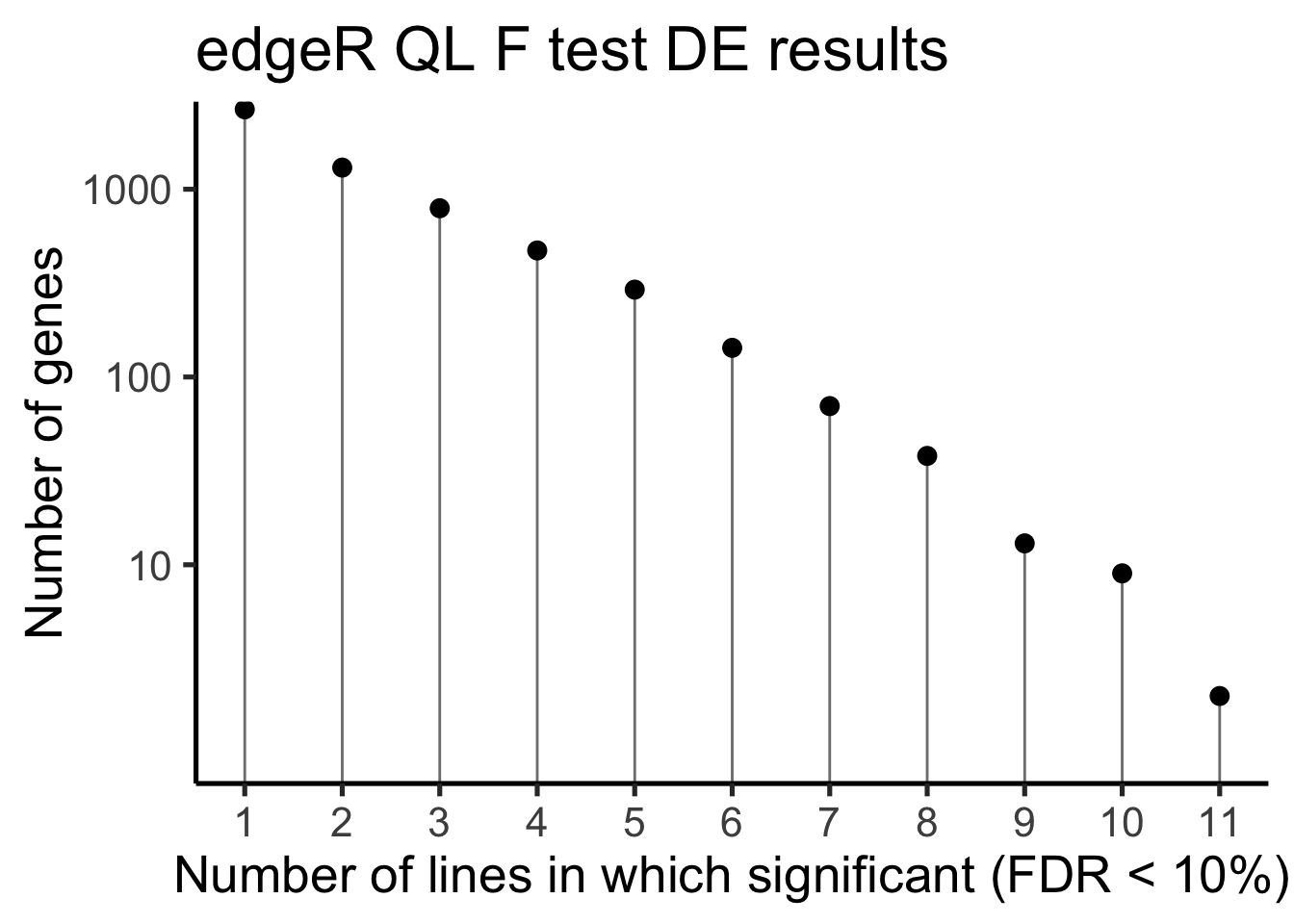

Expand here to see past versions of genewise-de-1.png:

Version	Author	Date
d2e8b31	davismcc	2018-08-19

ggsave("figures/differential_expression/alldonors_de_n_sig_donors_n_sig_genes.png", 
       height = 7, width = 10)
ggsave("figures/differential_expression/alldonors_de_n_sig_donors_n_sig_genes.pdf", 
       height = 7, width = 10)
ggsave("figures/differential_expression/alldonors_de_n_sig_donors_n_sig_genes.svg", 
       height = 7, width = 10)
       
p1 <- df_de_sig_unst %>% 
    group_by(gene) %>% 
    dplyr::mutate(id = paste0(donor, gene)) %>% distinct(id, .keep_all = TRUE) %>%
    dplyr::summarise(n_donors = n()) %>% group_by(n_donors) %>%
    dplyr::summarise(count = n()) %>%
ggplot(aes(x = n_donors, y = count)) +
    geom_segment(aes(x = n_donors, xend = n_donors, y = count, yend = 0.1), 
                 colour = "gray50") +
        geom_point(size = 3) +
    scale_x_continuous(breaks = 0:11) +
    #coord_cartesian(ylim = c(1, 2200)) +
    theme_classic(16) +
    xlab("Number of lines significant (FDR < 10%)")  +
    ylab("Number of genes")
p1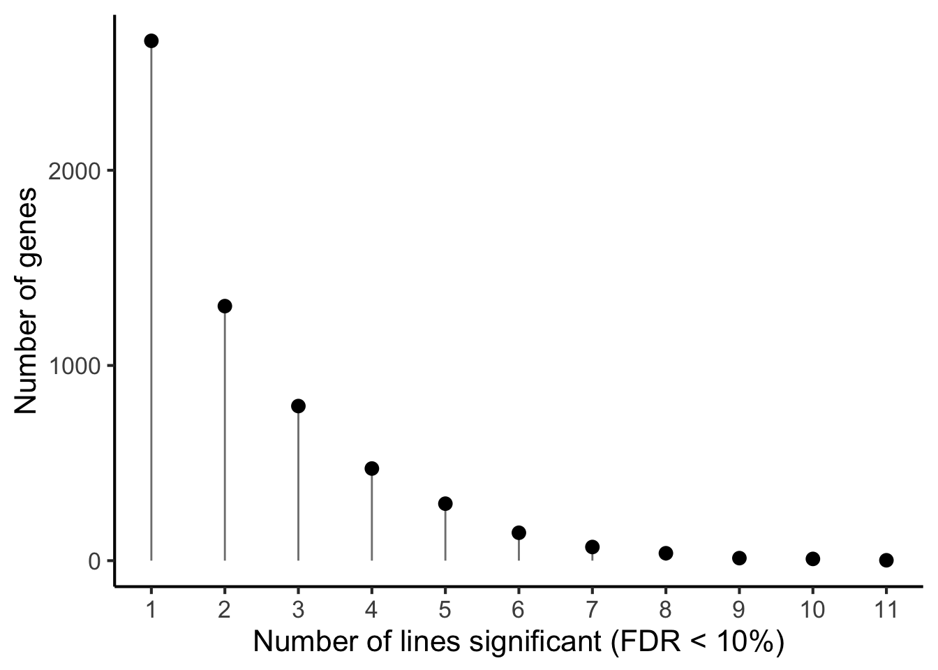

Expand here to see past versions of genewise-de-2.png:

Version	Author	Date
d2e8b31	davismcc	2018-08-19

ggsave("figures/differential_expression/alldonors_de_n_sig_donors_n_sig_genes_linscale.png", 
       height = 7, width = 5.5)
ggsave("figures/differential_expression/alldonors_de_n_sig_donors_n_sig_genes_linscale.pdf", 
       height = 7, width = 5.5)
ggsave("figures/differential_expression/alldonors_de_n_sig_donors_n_sig_genes_linscale.svg", 
       height = 7, width = 5.5)

p2 <- df_de_sig_unst %>% 
    group_by(gene) %>% 
    dplyr::mutate(id = paste0(donor, gene)) %>% distinct(id, .keep_all = TRUE) %>%
    dplyr::summarise(n_donors = n()) %>% dplyr::arrange(gene, n_donors) %>% ungroup() %>%
    dplyr::mutate(gene = gsub("ENSG.*_", "", gene)) %>%
    dplyr::filter(n_donors > 7.5) %>%
    ggplot(aes(y = n_donors, x = reorder(gene, n_donors, max))) +
    geom_point(alpha = 0.7, size = 4) +
    scale_y_continuous(breaks = 7:11) +
    ggthemes::scale_colour_tableau() +
    coord_flip() +
    theme_bw(16) +
    xlab("Gene") + ylab("Number of lines significant")
p2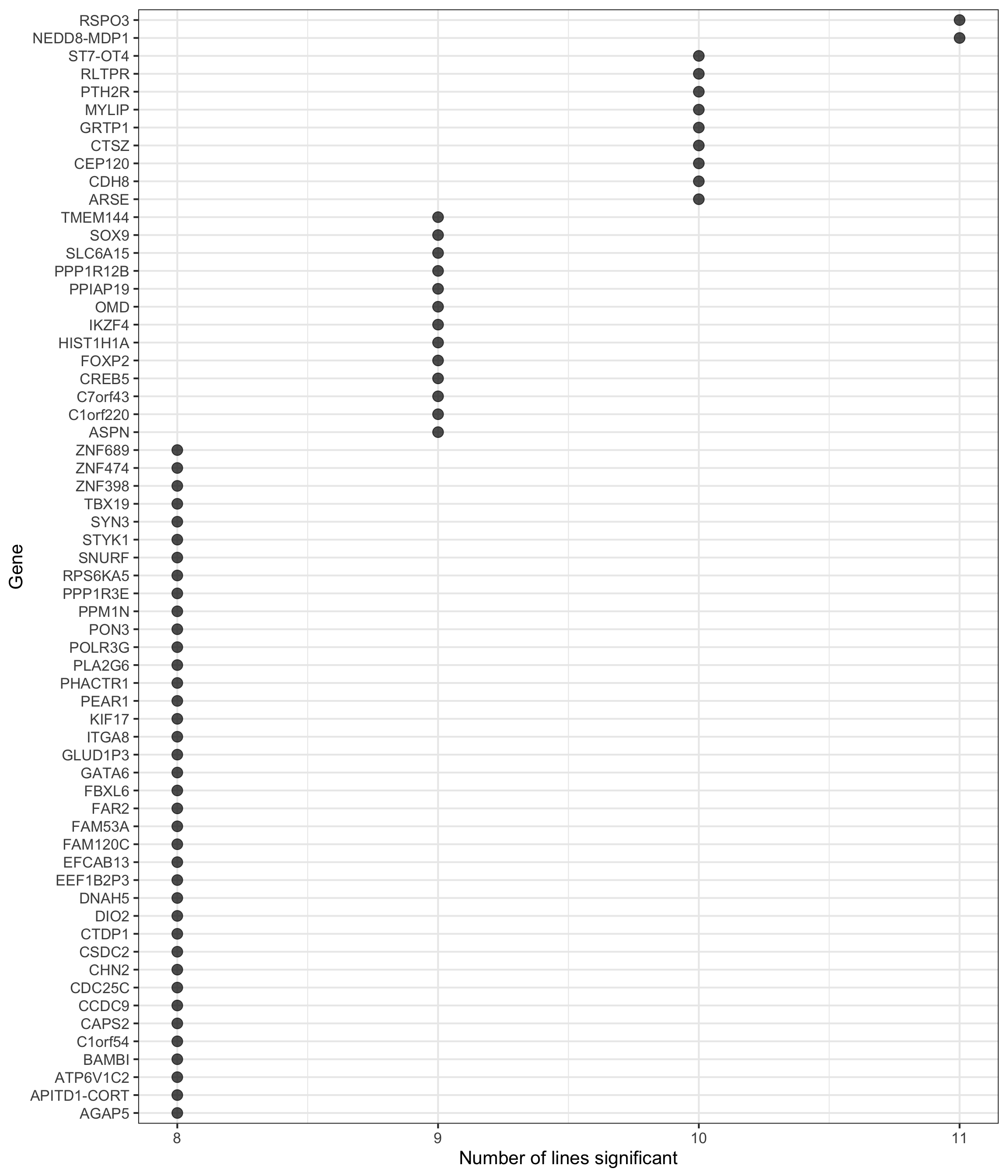

Expand here to see past versions of unnamed-chunk-1-1.png:

Version	Author	Date
d2e8b31	davismcc	2018-08-19

ggsave("figures/differential_expression/alldonors_de_n_sig_donors_topgenes.png", 
       height = 7, width = 5.5)
ggsave("figures/differential_expression/alldonors_de_n_sig_donors_topgenes.pdf", 
       height = 7, width = 5.5)
ggsave("figures/differential_expression/alldonors_de_n_sig_donors_topgenes.svg", 
       height = 7, width = 5.5)


#cowplot::plot_grid(p1, p2, rel_heights = c(0.4, 0.6))


df_donor_n_de <- df_de_sig_unst %>% 
    group_by(gene) %>% 
    dplyr::mutate(id = paste0(donor, gene)) %>% distinct(id, .keep_all = TRUE) %>%
    group_by(donor) %>%
    dplyr::summarise(count = n())
no_de_donor <- unique(df_de_all_unst[["donor"]])[!(unique(df_de_all_unst[["donor"]]) %in% df_donor_n_de[["donor"]])]
df_donor_n_de <- rbind(df_donor_n_de, data_frame(donor = no_de_donor, count = 0))

Permute gene labels to get a null distribution.

df_de_nsig <- df_de_all_unst %>% dplyr::filter(FDR < 0.1) %>% 
    dplyr::mutate(id = paste0(donor, gene)) %>% distinct(id, .keep_all = TRUE) %>%
    group_by(donor) %>% 
    dplyr::summarise(n_sig = n())
df_nsig_ncells_de <- full_join(df_ncells_de, df_de_nsig)
df_nsig_ncells_de$n_sig[is.na(df_nsig_ncells_de$n_sig)] <- 0

permute_gene_labels <- function(gene_names, n_de)  {
    sampled_genes <- c()
    for (i in seq_along(n_de))
        sampled_genes <- c(sampled_genes, sample(gene_names, size = n_de[i]))
    tab <- table(table(sampled_genes))
    df <- data_frame(n_donors = 1:11, n_genes = 0)
    df[names(tab), 2] <- tab
    df
}


n_perm <- 1000
df_perm <- list()
for (i in seq_len(n_perm))
    df_perm[[i]] <- permute_gene_labels(rownames(de_res$qlf_list$vass$table), 
                                        df_nsig_ncells_de[["n_sig"]])
df_perm <- do.call("rbind", df_perm)
df_perm <- dplyr::mutate(df_perm, data_type = "permuted")

df_perm %>% group_by(n_donors) %>% dplyr::summarise(min = min(n_genes), 
                                             median = median(n_genes),
                                             mean = mean(n_genes), 
                                             max = max(n_genes))

# A tibble: 11 x 5
   n_donors   min median     mean   max
      <int> <dbl>  <dbl>    <dbl> <dbl>
 1        1  3946   4120 4121.     4292
 2        2  2356   2466 2468.     2578
 3        3   821    897  896.      976
 4        4   177    223  223.      269
 5        5    23     40   40.3      59
 6        6     0      5    5.63     14
 7        7     0      0    0.595     4
 8        8     0      0    0.062     2
 9        9     0      0    0.007     1
10       10     0      0    0         0
11       11     0      0    0         0

ppp <- df_de_sig_unst %>% 
    group_by(gene) %>% 
    dplyr::mutate(id = paste0(donor, gene)) %>% distinct(id, .keep_all = TRUE) %>%
    dplyr::summarise(n_donors = n()) %>% group_by(n_donors) %>%
    dplyr::summarise(n_genes = n()) %>% dplyr::mutate(data_type = "observed") %>%
ggplot(aes(x = n_donors, y = n_genes)) +
    # geom_segment(aes(x = n_donors, xend = n_donors, y = count, yend = 0.1), 
    #              colour = "gray50") +
#    geom_hline(yintercept = 0, linetype = 2) +
    geom_hline(yintercept = 0) +
    geom_boxplot(aes(group = n_donors, y = n_genes, colour = data_type), 
                 fill = "gray80", data = df_perm, show.legend = FALSE) +
    geom_point(aes(colour = data_type), shape = 17, size = 5) +
    scale_x_continuous(breaks = 0:11) +
    scale_y_sqrt(breaks = c(0, 10, 100, 500, 1000, 2000, 3000),
                 labels = c(0, 10, 100, 500, 1000, 2000, 3000),
                 limits = c(0, 4500)) +
    scale_colour_manual(name = '', 
                        values = c("observed" = "black", "permuted" = "gray50"), 
                        labels = c("observed", "permuted")) +
    coord_cartesian(ylim = c(0, 4500)) +
    theme_bw(18) +
    theme(legend.position = c(0.8, 0.88),
          panel.grid.major.x = element_blank(), 
          panel.grid.minor.x = element_blank()) +
    guides(colour = guide_legend(override.aes = list(shape = c(17, 19))),
           fill = FALSE, boxplot = FALSE) +
    xlab("Number of lines significant (FDR < 10%)")  +
    ylab("Number of genes")

ggsave("figures/differential_expression/alldonors_de_n_sig_donors_n_sig_genes_sqrtscale_perm.png", 
       height = 7, width = 10, plot = ppp)
ggsave("figures/differential_expression/alldonors_de_n_sig_donors_n_sig_genes_sqrtscale_perm.pdf", 
       height = 7, width = 10, plot = ppp)
ggsave("figures/differential_expression/alldonors_de_n_sig_donors_n_sig_genes_sqrtscale_perm.svg", 
       height = 7, width = 10, plot = ppp)

df_de_sig_unst %>% 
    group_by(gene) %>% 
    dplyr::mutate(id = paste0(donor, gene)) %>% distinct(id, .keep_all = TRUE) %>%
    dplyr::summarise(n_donors = n()) %>% group_by(n_donors) %>%
    dplyr::summarise(n_genes = n()) %>% dplyr::mutate(data_type = "observed") %>%
ggplot(aes(x = n_donors, y = n_genes)) +
    # geom_segment(aes(x = n_donors, xend = n_donors, y = count, yend = 0.1), 
    #              colour = "gray50") +
#    geom_hline(yintercept = 0, linetype = 2) +
    geom_hline(yintercept = 0) +
    geom_boxplot(aes(group = n_donors, y = n_genes, colour = data_type), 
                 fill = "gray80", data = df_perm, show.legend = FALSE) +
    geom_point(aes(colour = data_type), shape = 17, size = 5) +
    scale_x_continuous(breaks = 0:11) +
    scale_y_sqrt(breaks = c(0, 10, 100, 500, 1000, 2000, 3000),
                 labels = c(0, 10, 100, 500, 1000, 2000, 3000),
                 limits = c(0, 4500)) +
    scale_colour_manual(name = '', 
                        values = c("observed" = "black", "permuted" = "gray50"), 
                        labels = c("observed", "permuted")) +
    coord_cartesian(ylim = c(0, 4500)) +
    theme(legend.position = c(0.8, 0.88),
          panel.grid.major.x = element_blank(), 
          panel.grid.minor.x = element_blank()) +
    guides(colour = guide_legend(override.aes = list(shape = c(17, 19))),
           fill = FALSE, boxplot = FALSE) +
    xlab("Number of lines significant (FDR < 10%)")  +
    ylab("Number of genes")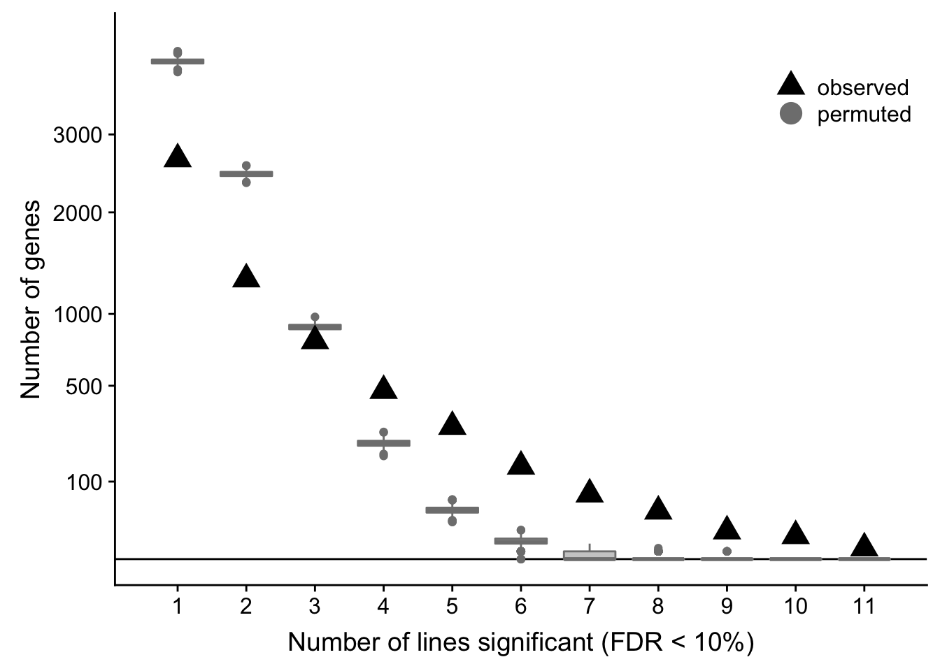

Expand here to see past versions of permute-de-1.png:

Version	Author	Date
d2e8b31	davismcc	2018-08-19

ggsave("figures/differential_expression/alldonors_de_n_sig_donors_n_sig_genes_sqrtscale_perm_skinny.png", 
       height = 5.5, width = 6.5)

ggsave("figures/differential_expression/alldonors_de_n_sig_donors_n_sig_genes_sqrtscale_perm_veryskinny.png", 
       height = 7.5, width = 6.5)

Look at recurrently DE genes.

df_gene_n_de <- df_de_sig_unst %>% 
    group_by(gene) %>% 
    dplyr::mutate(id = paste0(donor, gene)) %>% distinct(id, .keep_all = TRUE) %>%
    group_by(gene) %>%
    dplyr::summarise(count = n()) %>% 
    dplyr::arrange(desc(count)) %>%
    dplyr::mutate(ensembl_gene_id = gsub("_.*", "", gene),
                  hgnc_symbol = gsub(".*_", "", gene))
df_gene_n_de <- left_join(
    df_gene_n_de,
    dplyr::select(de_res$qlf_pairwise$joxm$clone2_clone1$table, 
                  ensembl_gene_id, hgnc_symbol, entrezid)
    )
df_gene_n_de <- dplyr::mutate(
    df_gene_n_de,
    cell_cycle_growth = (entrezid %in% 
                             c(Hs.H$HALLMARK_G2M_CHECKPOINT,
                               Hs.H$HALLMARK_MITOTIC_SPINDLE,
                               Hs.H$HALLMARK_E2F_TARGETS)),
    myc = (entrezid %in% c(Hs.H$HALLMARK_MYC_TARGETS_V1,
                           Hs.H$HALLMARK_MYC_TARGETS_V2)),
    emt = (entrezid %in% c(Hs.H$HALLMARK_EPITHELIAL_MESENCHYMAL_TRANSITION))
)
df_gene_n_de %>% dplyr::filter(count >= 8) %>% 
  DT::datatable(.)

Camera results

First, aggregate gene set enrichment results across all donors.

fdr_thresh <- 1
df_camera_all_unst <- data_frame()
for (geneset in names(de_res[["camera"]])) {
    for (donor in names(de_res[["camera"]][[geneset]])) {
        for (coeff in names(de_res[["camera"]][[geneset]][[donor]])) {
            for (stat in names(de_res[["camera"]][[geneset]][[donor]][[coeff]])) {
                tmp <- de_res[["camera"]][[geneset]][[donor]][[coeff]][[stat]]
                tmp <- tmp[tmp$FDR <= fdr_thresh,]
                if (nrow(tmp) > 0.5) {
                    tmp[["collection"]] <- geneset
                    tmp[["geneset"]] <- rownames(tmp)
                    tmp[["coeff"]] <- coeff
                    tmp[["donor"]] <- donor
                    tmp[["stat"]] <- stat
                    df_camera_all_unst <- bind_rows(df_camera_all_unst, tmp)
                }
            }
        }
    }
}

fdr_thresh <- 0.05
df_camera_sig_unst <- data_frame()
for (geneset in names(de_res[["camera"]])) {
    for (donor in names(de_res[["camera"]][[geneset]])) {
        for (coeff in names(de_res[["camera"]][[geneset]][[donor]])) {
            for (stat in names(de_res[["camera"]][[geneset]][[donor]][[coeff]])) {
                tmp <- de_res[["camera"]][[geneset]][[donor]][[coeff]][[stat]]
                tmp <- tmp[tmp$FDR <= fdr_thresh,]
                if (nrow(tmp) > 0.5) {
                    tmp[["collection"]] <- geneset
                    tmp[["geneset"]] <- rownames(tmp)
                    tmp[["coeff"]] <- coeff
                    tmp[["donor"]] <- donor
                    tmp[["stat"]] <- stat
                    df_camera_sig_unst <- bind_rows(df_camera_sig_unst, tmp)
                }
            }
        }
    }
}

df_camera_sig_unst <- dplyr::mutate(
    df_camera_sig_unst,
    contrast = gsub("_", " - ", coeff),
    msigdb_collection = plyr::mapvalues(collection, from = c("c2", "c6", "H"), to = c("MSigDB curated (c2)", "MSigDB oncogenic (c6)", "MSigDB Hallmark")))

df_camera_all_unst <- dplyr::mutate(
    df_camera_all_unst,
    contrast = gsub("_", " - ", coeff),
    msigdb_collection = plyr::mapvalues(collection, from = c("c2", "c6", "H"), to = c("MSigDB curated (c2)", "MSigDB oncogenic (c6)", "MSigDB Hallmark")))

We now have a dataframe for significant (FDR <5%) results from the camera gene set enrichment results.

head(df_camera_sig_unst)

# A tibble: 6 x 11
  NGenes Direction   PValue      FDR collection geneset coeff donor stat 
   <dbl> <chr>        <dbl>    <dbl> <chr>      <chr>   <chr> <chr> <chr>
1      6 Down      6.43e-15 3.02e-11 c2         VALK_A… clon… euts  signF
2      7 Down      2.29e-11 5.37e- 8 c2         WANG_R… clon… euts  signF
3      5 Down      7.80e-11 1.22e- 7 c2         GUTIER… clon… euts  signF
4      8 Down      1.35e- 9 1.58e- 6 c2         KUMAMO… clon… euts  signF
5     11 Down      4.95e- 9 4.65e- 6 c2         VALK_A… clon… euts  signF
6      4 Down      2.86e- 8 1.92e- 5 c2         REACTO… clon… euts  signF
# ... with 2 more variables: contrast <chr>, msigdb_collection <chr>

And a dataframe with all results.

head(df_camera_all_unst)

# A tibble: 6 x 11
  NGenes Direction  PValue   FDR collection geneset coeff donor stat 
   <dbl> <chr>       <dbl> <dbl> <chr>      <chr>   <chr> <chr> <chr>
1      7 Down      2.88e-4 0.771 c2         WANG_R… clon… euts  logFC
2     10 Down      4.73e-4 0.771 c2         BIOCAR… clon… euts  logFC
3     15 Up        8.30e-4 0.771 c2         LI_CIS… clon… euts  logFC
4     14 Down      1.07e-3 0.771 c2         MOROSE… clon… euts  logFC
5      5 Down      1.12e-3 0.771 c2         IYENGA… clon… euts  logFC
6     15 Up        1.19e-3 0.771 c2         PID_TC… clon… euts  logFC
# ... with 2 more variables: contrast <chr>, msigdb_collection <chr>

For now, focus on gene set enrichment results computed using log-fold change statistics for pairwise comparisons of clones estimated from the edgeR QL-F models.

We can look at all significant results summarised by donor, geneset and pairwise contrast of clones.

df_camera_sig_unst %>% 
    dplyr::filter(stat == "logFC") %>%
    dplyr::mutate(donor = factor(donor, levels = rev(levels(factor(donor))))) %>%
ggplot(aes(y = -log10(PValue), x = donor, colour = contrast)) +
    geom_sina(alpha = 0.7) +
    facet_grid(contrast ~ msigdb_collection) + 
    scale_colour_brewer(palette = "Accent") +
    coord_flip() + theme_bw()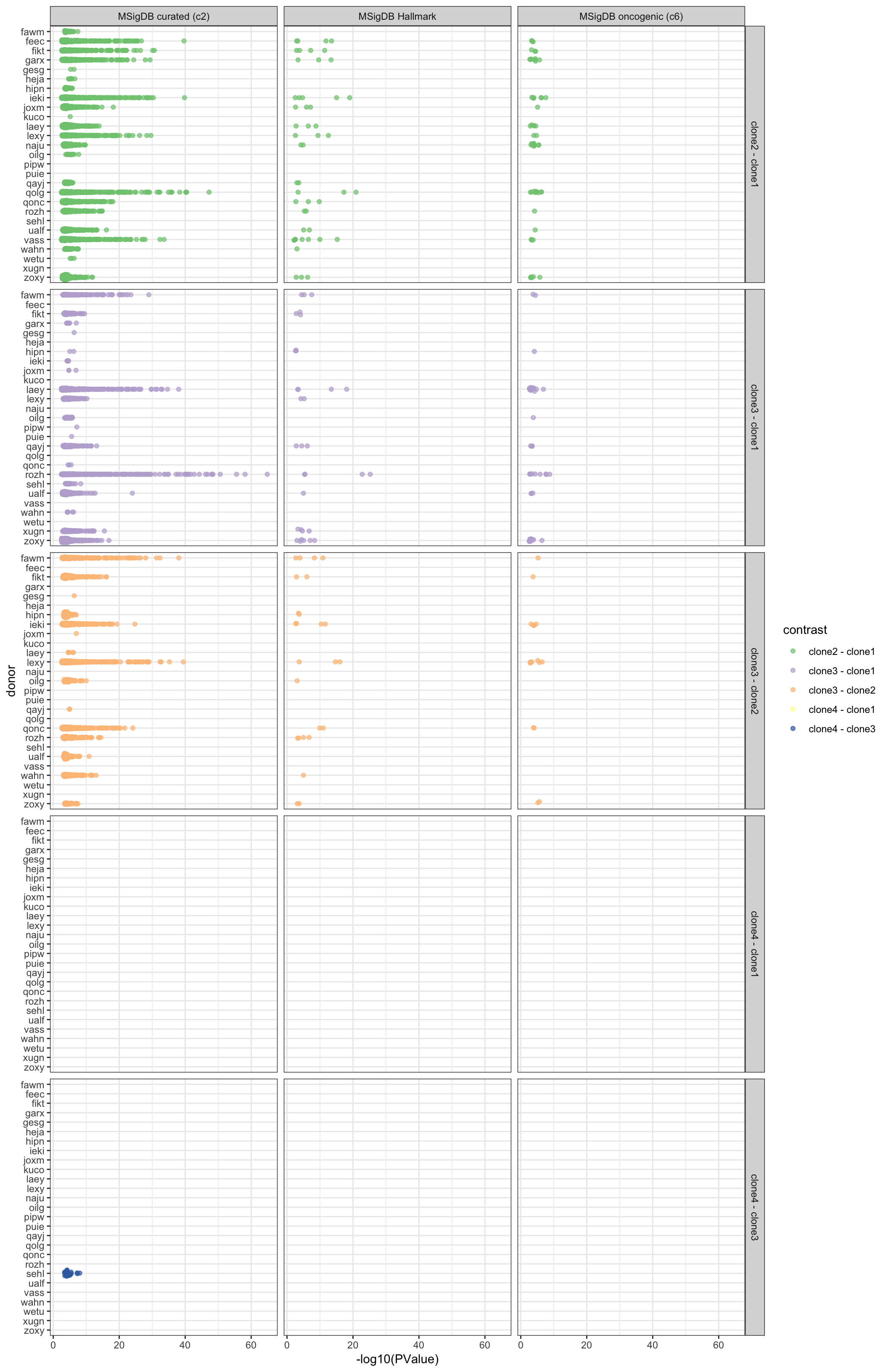

Expand here to see past versions of camera-allcontr-allsets-sig-bydonor-pvals-1.png:

Version	Author	Date
d2e8b31	davismcc	2018-08-19

Similarly, we can look at all results summarised by donor, geneset and pairwise contrast of clones.

df_camera_all_unst %>%
    dplyr::filter(stat == "logFC") %>%
    dplyr::mutate(donor = factor(donor, levels = rev(levels(factor(donor))))) %>%
ggplot(aes(y = -log10(FDR), x = donor, colour = contrast)) +
    geom_sina(alpha = 0.7) +
    geom_hline(yintercept = -log10(0.05), linetype = 2, colour = "firebrick") +
    facet_grid(contrast ~ msigdb_collection, scales = "free_x") + 
    scale_colour_brewer(palette = "Accent") +
    coord_flip() + theme_bw()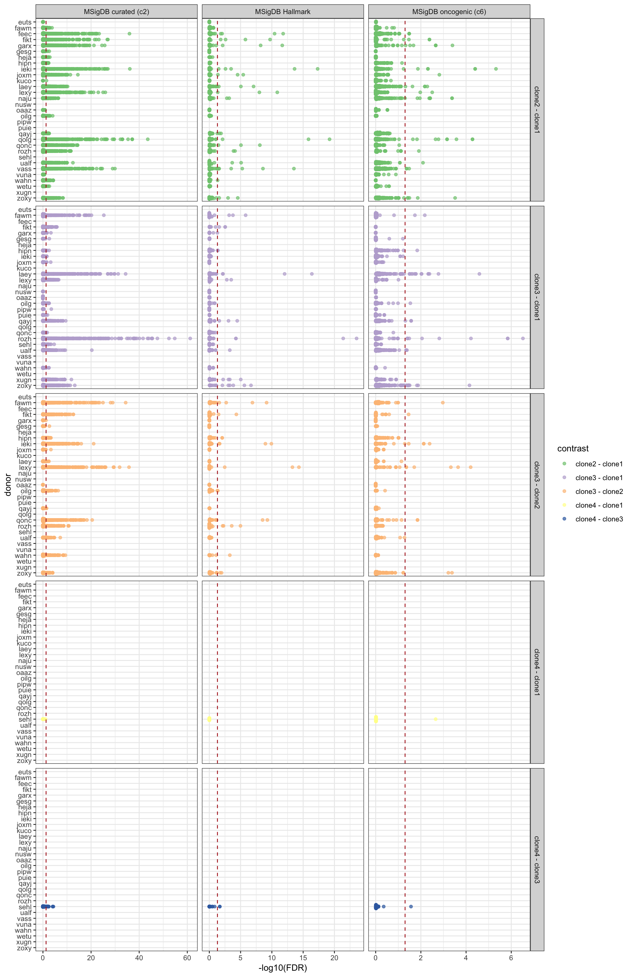

Expand here to see past versions of camera-allcontr-allsets-all-bydonor-fdr-1.png:

Version	Author	Date
d2e8b31	davismcc	2018-08-19

ggsave("figures/differential_expression/alldonors_camera_enrichment_by_donor_all_results.png", 
       height = 16, width = 14)
ggsave("figures/differential_expression/alldonors_camera_enrichment_by_donor_all_results.pdf", 
       height = 16, width = 14)
ggsave("figures/differential_expression/alldonors_camera_enrichment_by_donor_all_results.svg", 
       height = 16, width = 14)

We can check the number of significant gene sets for each donor, for each MSigDB gene set collection.

df_camera_sig_unst %>% 
    dplyr::filter(stat == "logFC") %>%
    dplyr::filter(FDR < 0.05) %>%
    group_by(donor, msigdb_collection) %>%
    dplyr::summarise(n_sig = n()) %>% print(n = Inf)

# A tibble: 67 x 3
# Groups:   donor [?]
   donor msigdb_collection     n_sig
   <chr> <chr>                 <int>
 1 fawm  MSigDB curated (c2)     348
 2 fawm  MSigDB Hallmark           7
 3 fawm  MSigDB oncogenic (c6)     3
 4 feec  MSigDB curated (c2)     256
 5 feec  MSigDB Hallmark           4
 6 feec  MSigDB oncogenic (c6)     3
 7 fikt  MSigDB curated (c2)     426
 8 fikt  MSigDB Hallmark           9
 9 fikt  MSigDB oncogenic (c6)     4
10 garx  MSigDB curated (c2)     244
11 garx  MSigDB Hallmark           3
12 garx  MSigDB oncogenic (c6)     7
13 gesg  MSigDB curated (c2)       4
14 heja  MSigDB curated (c2)       7
15 hipn  MSigDB curated (c2)      99
16 hipn  MSigDB Hallmark           5
17 hipn  MSigDB oncogenic (c6)     1
18 ieki  MSigDB curated (c2)     480
19 ieki  MSigDB Hallmark           9
20 ieki  MSigDB oncogenic (c6)    10
21 joxm  MSigDB curated (c2)     150
22 joxm  MSigDB Hallmark           3
23 joxm  MSigDB oncogenic (c6)     1
24 kuco  MSigDB curated (c2)       1
25 laey  MSigDB curated (c2)     502
26 laey  MSigDB Hallmark           7
27 laey  MSigDB oncogenic (c6)    19
28 lexy  MSigDB curated (c2)     546
29 lexy  MSigDB Hallmark           8
30 lexy  MSigDB oncogenic (c6)     8
31 naju  MSigDB curated (c2)      99
32 naju  MSigDB Hallmark           2
33 naju  MSigDB oncogenic (c6)    10
34 oilg  MSigDB curated (c2)     102
35 oilg  MSigDB Hallmark           1
36 oilg  MSigDB oncogenic (c6)     1
37 pipw  MSigDB curated (c2)       1
38 puie  MSigDB curated (c2)       1
39 qayj  MSigDB curated (c2)     152
40 qayj  MSigDB Hallmark           5
41 qayj  MSigDB oncogenic (c6)     4
42 qolg  MSigDB curated (c2)     293
43 qolg  MSigDB Hallmark           3
44 qolg  MSigDB oncogenic (c6)     9
45 qonc  MSigDB curated (c2)     382
46 qonc  MSigDB Hallmark           5
47 qonc  MSigDB oncogenic (c6)     2
48 rozh  MSigDB curated (c2)     553
49 rozh  MSigDB Hallmark          10
50 rozh  MSigDB oncogenic (c6)    10
51 sehl  MSigDB curated (c2)      59
52 sehl  MSigDB Hallmark           2
53 sehl  MSigDB oncogenic (c6)     2
54 ualf  MSigDB curated (c2)     378
55 ualf  MSigDB Hallmark           3
56 ualf  MSigDB oncogenic (c6)     4
57 vass  MSigDB curated (c2)     270
58 vass  MSigDB Hallmark           8
59 vass  MSigDB oncogenic (c6)     3
60 wahn  MSigDB curated (c2)     129
61 wahn  MSigDB Hallmark           2
62 wetu  MSigDB curated (c2)       3
63 xugn  MSigDB curated (c2)     120
64 xugn  MSigDB Hallmark           4
65 zoxy  MSigDB curated (c2)     488
66 zoxy  MSigDB Hallmark          11
67 zoxy  MSigDB oncogenic (c6)    19

We can look at the number of significant gene sets for each donor.

## simpler version
df_camera_all_unst %>% 
    dplyr::filter(stat == "logFC") %>%
    group_by(donor, msigdb_collection) %>%
    dplyr::summarise(n_sig = sum(FDR < 0.05)) %>% ungroup() %>% 
    dplyr::mutate(donor = factor(donor, levels = rev(levels(factor(donor))))) %>%
    ggplot(aes(y = n_sig, x = donor)) +
    geom_point(alpha = 1, size = 4) +
    facet_wrap(~ msigdb_collection, scales = "free_x") + 
    scale_fill_brewer(palette = "Accent") +
    coord_flip() +
    theme_bw(16) +
    xlab("Donor") + ylab("Number of significant genesets (FDR < 5%)") +
    ggtitle("Camera MSigDB gene set enrichment by line")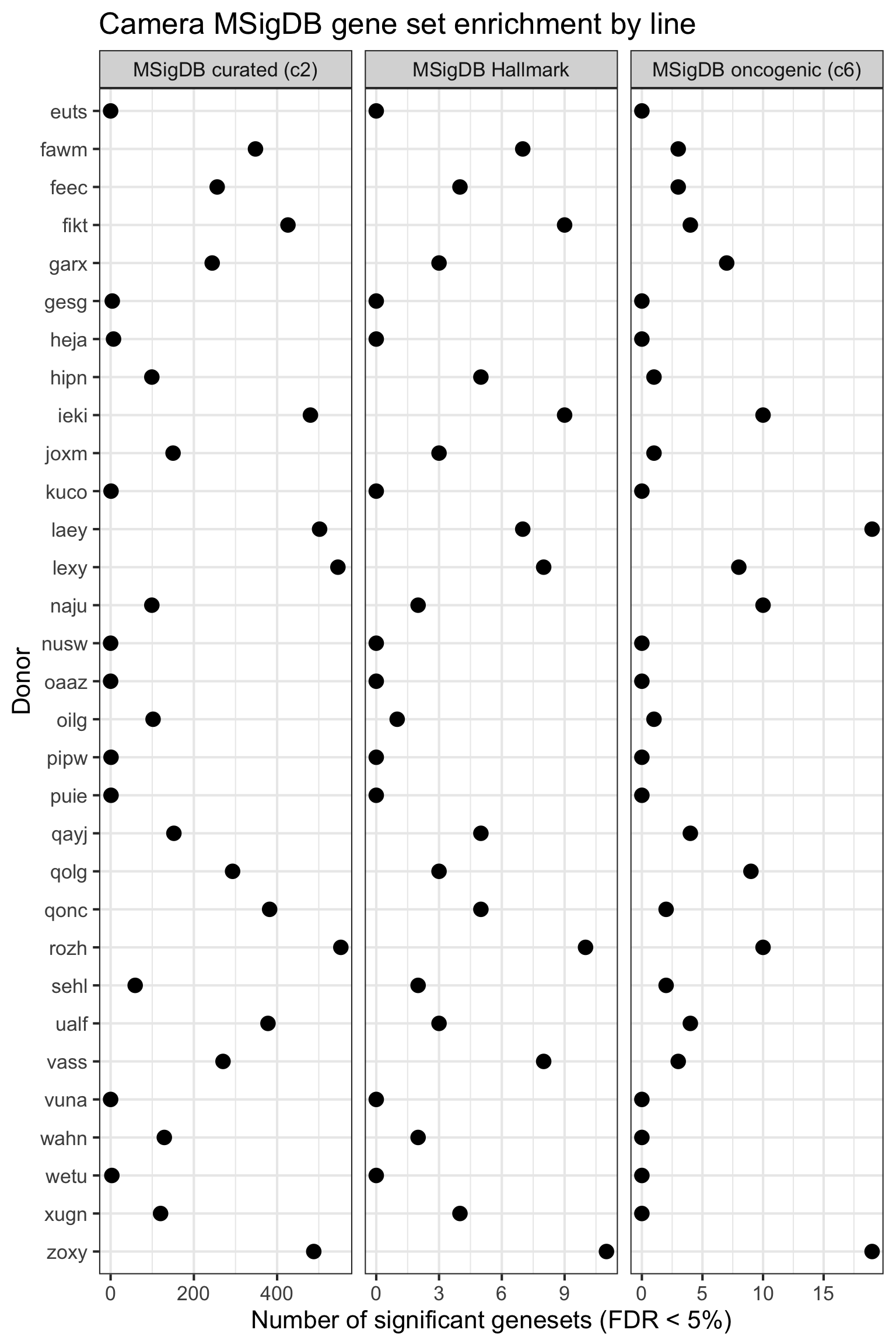

Expand here to see past versions of alldonors_camera_enrichment_by_donor_simple-1.png:

Version	Author	Date
d2e8b31	davismcc	2018-08-19

ggsave("figures/differential_expression/alldonors_camera_enrichment_by_donor_simple.png", 
       height = 7, width = 10)
ggsave("figures/differential_expression/alldonors_camera_enrichment_by_donor_simple.pdf", 
       height = 7, width = 10)
ggsave("figures/differential_expression/alldonors_camera_enrichment_by_donor_simple.svg", 
       height = 7, width = 10)

We can look at the effect of the the number of cells for each donor on the DE results obtained.

ncells_by_donor <- rep(NA, length(sce_unst_list))
names(ncells_by_donor) <- names(sce_unst_list)
for (don in names(sce_unst_list))
    ncells_by_donor[don] <- ncol(sce_unst_list[[don]])

df_camera_all_unst %>% 
    dplyr::filter(stat == "logFC") %>%
    group_by(donor, msigdb_collection) %>%
    dplyr::summarise(n_sig = sum(FDR < 0.05)) %>% ungroup() -> df_to_plot
df_to_plot <- inner_join(df_to_plot, 
                        data_frame(donor = names(ncells_by_donor),
                                   ncells = ncells_by_donor))
df_to_plot %>%
    dplyr::mutate(donor = factor(donor, levels = rev(levels(factor(donor))))) %>%
    ggplot(aes(y = n_sig, x = donor, size = ncells)) +
    geom_point(alpha = 1) +
    facet_wrap(~ msigdb_collection, scales = "free_x") + 
    scale_fill_brewer(palette = "Accent") +
    coord_flip() +
    theme_bw(16) +
    xlab("Donor") + ylab("Number of significant genesets (FDR < 5%)") +
    ggtitle("Camera MSigDB gene set enrichment by line")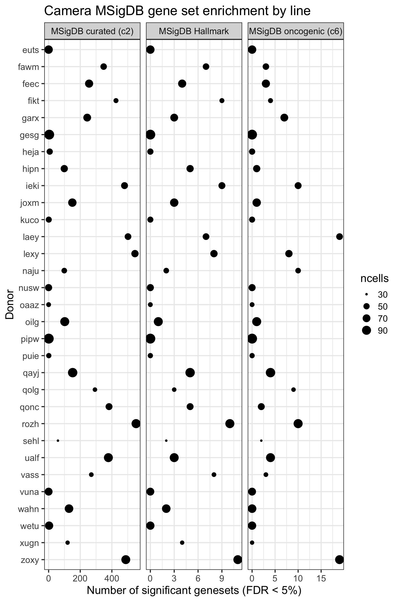

Expand here to see past versions of alldonors_camera_enrichment_by_donor_simple_size_by_ncells-1.png:

Version	Author	Date
d2e8b31	davismcc	2018-08-19

ggsave("figures/differential_expression/alldonors_camera_enrichment_by_donor_simple_size_by_ncells.png", 
       height = 7, width = 10)
ggsave("figures/differential_expression/alldonors_camera_enrichment_by_donor_simple_size_by_ncells.pdf", 
       height = 7, width = 10)
ggsave("figures/differential_expression/alldonors_camera_enrichment_by_donor_simple_size_by_ncells.svg", 
       height = 7, width = 10)

Hallmark gene set

Focus now on looking at DE results for the MSigDB Hallmark gene set (50 of the best-characterised gene sets as determined by MSigDB).

Look at the gene sets that are found to be enriched in multiple donors.

## Hallmark geneset
df_camera_sig_unst %>% dplyr::filter(collection == "H") %>% 
    dplyr::filter(stat == "logFC") %>%
    group_by(geneset) %>% 
    dplyr::mutate(id = paste0(donor, geneset)) %>% distinct(id, .keep_all = TRUE) %>%
    dplyr::summarise(n_donors = n()) %>% dplyr::arrange(geneset, n_donors) %>% ungroup() %>%
    dplyr::mutate(geneset = gsub("_", " ", gsub("HALLMARK_", "", geneset))) %>%
ggplot(aes(y = n_donors, x = reorder(geneset, n_donors, max))) +
    geom_point(alpha = 0.7, size = 4) +
    ggthemes::scale_colour_tableau() +
    coord_flip() +
    theme_bw(14) +
    xlab("Gene set") + ylab("Number of lines significant")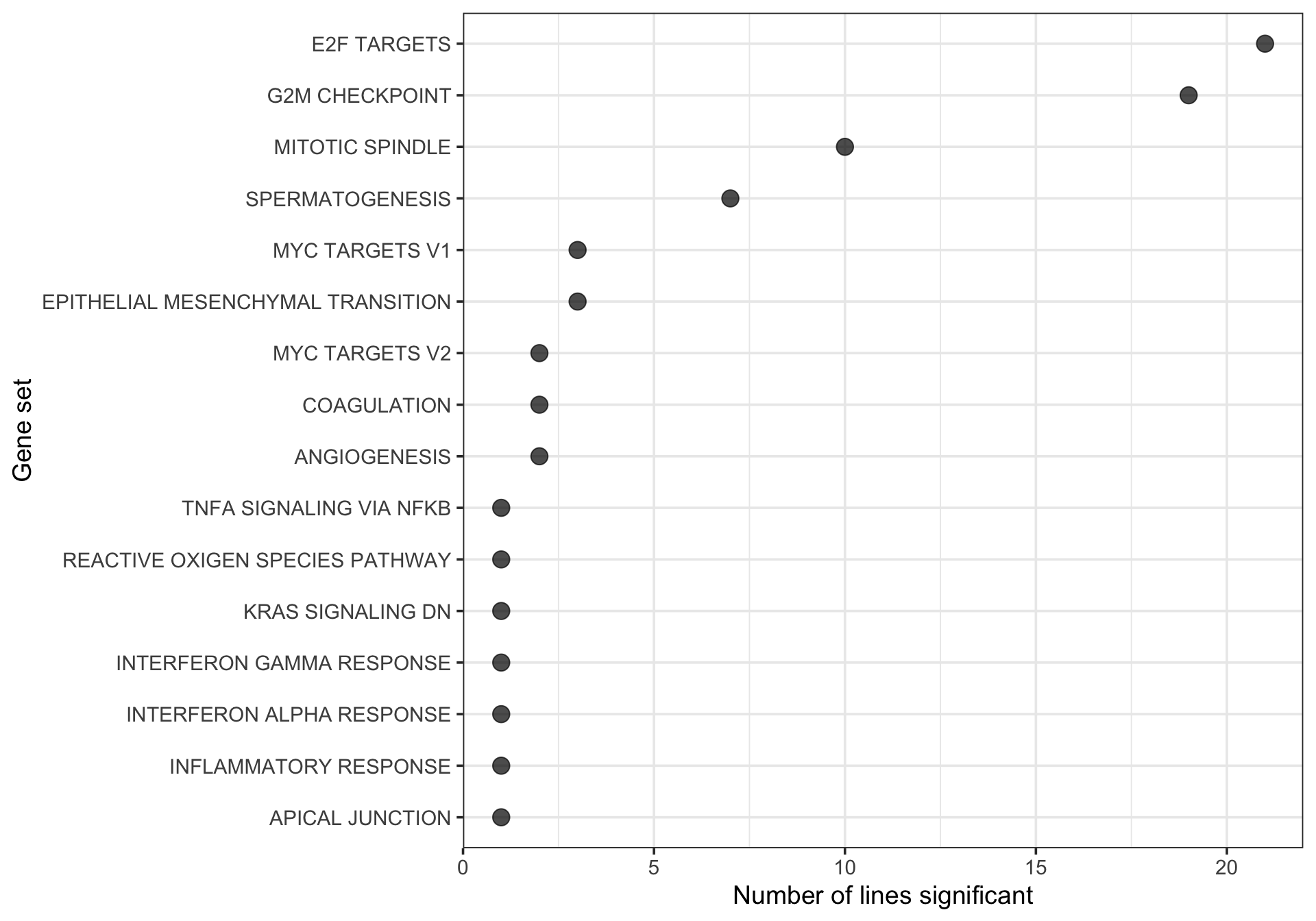

Expand here to see past versions of alldonors_camera_enrichment_H_by_geneset-1.png:

Version	Author	Date
d2e8b31	davismcc	2018-08-19

ggsave("figures/differential_expression/alldonors_camera_enrichment_H_by_geneset.png", 
       height = 7, width = 9.5)
ggsave("figures/differential_expression/alldonors_camera_enrichment_H_by_geneset.pdf", 
       height = 7, width = 9.5)
ggsave("figures/differential_expression/alldonors_camera_enrichment_H_by_geneset.svg", 
       height = 7, width = 9.5)
## number of donors with at least one significant geneset
tmp <- df_camera_sig_unst %>% dplyr::filter(collection == "H") %>% 
    dplyr::filter(stat == "logFC") %>%
    group_by(geneset)
unique(tmp[["donor"]])

 [1] "fawm" "feec" "fikt" "garx" "hipn" "ieki" "joxm" "laey" "lexy" "naju"
[11] "oilg" "qayj" "qolg" "qonc" "rozh" "sehl" "ualf" "vass" "wahn" "xugn"
[21] "zoxy"

21 donors have at least one significantly enriched Hallmark gene set.

For gene sets related directly to cell cycle and growth, we see contrasts being both up- and down- regulated, but for EMT, coagulation and angiogenesis pathways, we only see these down-regulated.

df_camera_sig_unst %>% dplyr::filter(collection == "H") %>% 
  dplyr::filter(stat == "logFC") %>%
  group_by(geneset, Direction) %>% 
  dplyr::mutate(id = paste0(donor, geneset)) %>% 
  dplyr::summarise(n_donors = n()) %>% dplyr::arrange(geneset, n_donors) %>% ungroup() %>%
  ggplot(aes(y = n_donors, x = reorder(geneset, n_donors, max),
             colour = Direction)) +
  geom_point(alpha = 0.7, size = 4, position = position_dodge(width = 0.5)) +
  ggthemes::scale_colour_tableau() +
  coord_flip() +
  theme_bw(16) +
  xlab("Gene set") + ylab("Number of lines significant")  +
  ggtitle("Camera MSigDB Hallmark gene set enrichment")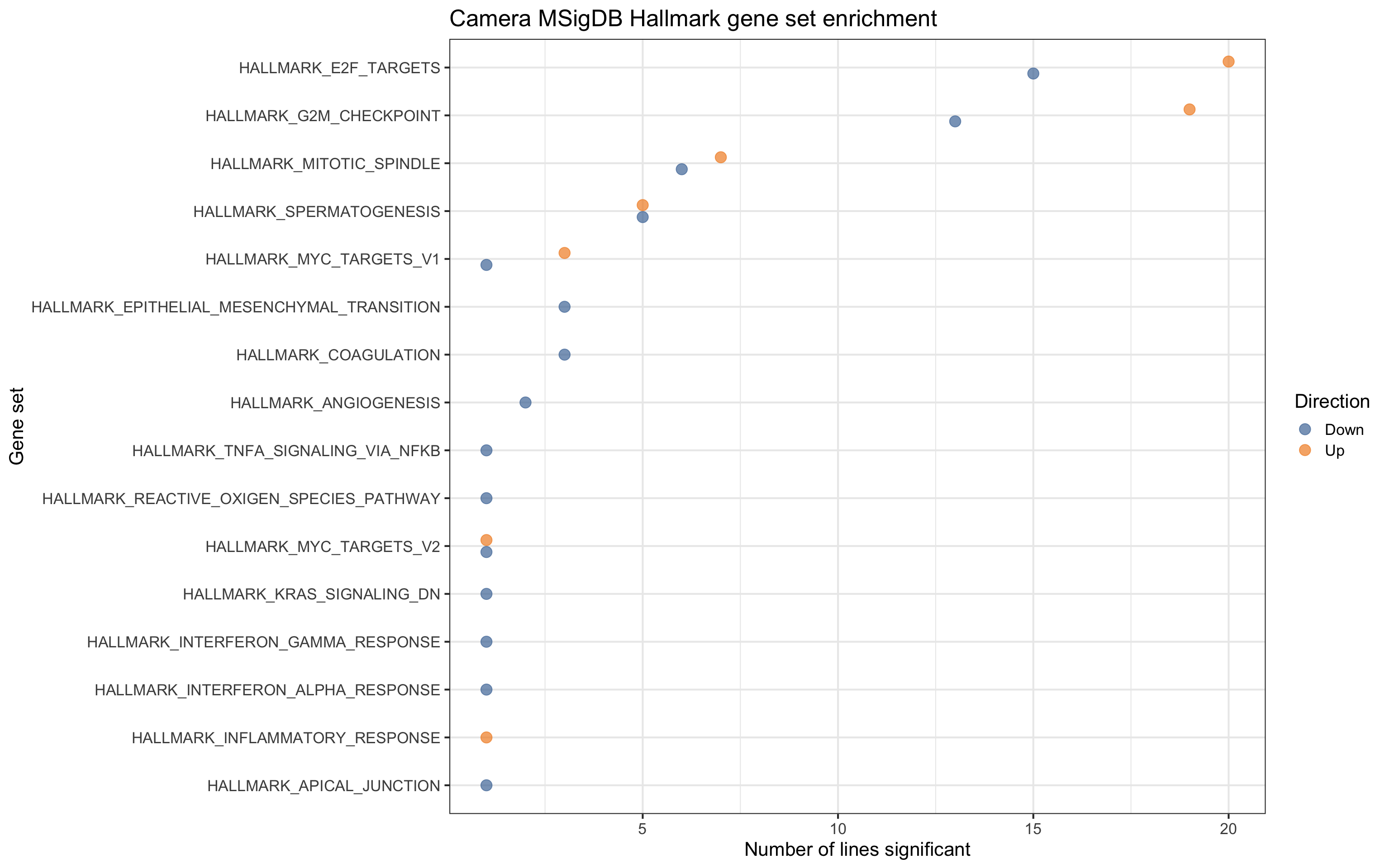

Expand here to see past versions of alldonors_camera_enrichment_H_by_geneset_by_dir-1.png:

Version	Author	Date
d2e8b31	davismcc	2018-08-19

Heatmap of results for camera Hallmark geneset testing

We can get an overview of all the Hallmark gene set results by producing a heatmap, first showing just the significant (FDR < 5%) results across all donors and pairwise contrasts of clones.

repeated_sig_H_genesets <- df_camera_sig_unst %>% 
    dplyr::filter(collection == "H", stat == "logFC") %>% 
    group_by(geneset) %>% 
    dplyr::mutate(id = paste0(donor, geneset)) %>% distinct(id, .keep_all = TRUE) %>%
    dplyr::summarise(n_donors = n()) %>% dplyr::arrange(n_donors) %>% 
    dplyr::filter(n_donors > 0.5) 
repeated_sig_H_genesets_vec <- unique(repeated_sig_H_genesets[["geneset"]])
repeated_sig_H_genesets_vec <- gsub("_", " ", gsub("HALLMARK_", "", 
                                                   repeated_sig_H_genesets_vec))
     
df_4_heatmap <- df_camera_sig_unst %>% 
  dplyr::filter(collection == "H", stat == "logFC") %>%
  dplyr::mutate(geneset = gsub("_", " ", gsub("HALLMARK_", "", geneset))) %>%
  dplyr::mutate(geneset = 
                  factor(geneset, levels = repeated_sig_H_genesets_vec)) %>%
  dplyr::filter(geneset %in% repeated_sig_H_genesets_vec) %>%
  dplyr::mutate(id = paste0(donor, ": ", contrast))
  

div_lines <- gsub(": c.*", "",
     sort(unique(paste0(df_4_heatmap[["donor"]], ": ", 
                        df_4_heatmap[["contrast"]])))) %>% table %>% cumsum + 0.5
    
df_4_heatmap %>%
    ggplot(aes(x = id, y = geneset, fill = Direction)) +
    geom_tile() +
    geom_vline(xintercept = div_lines, colour = "gray70") +
    scale_fill_manual(values = c("lightgoldenrod1", "sienna1")) +
    theme(axis.text.x = element_text(angle = 60, hjust = 1))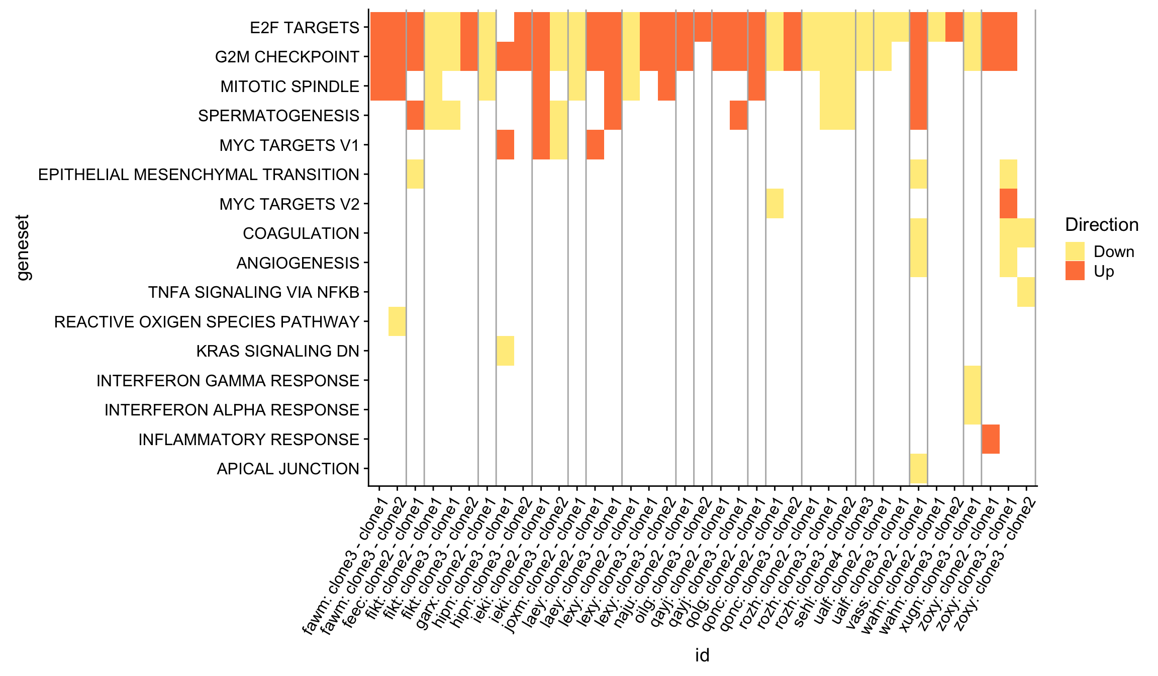

Expand here to see past versions of top_genesets_H_direction_heatmap-1.png:

Version	Author	Date
02a8343	davismcc	2018-08-24
d2e8b31	davismcc	2018-08-19

ggsave("figures/differential_expression/top_genesets_H_direction_heatmap.png", height = 6, width = 12)
ggsave("figures/differential_expression/top_genesets_H_direction_heatmap.pdf", height = 6, width = 12)
ggsave("figures/differential_expression/top_genesets_H_direction_heatmap.svg", height = 6, width = 12)

We can do the same for all results for the gene sets that are significantly enriched in at least two donors.

df_camera_all_unst %>% 
    dplyr::mutate(geneset = gsub("_", " ", gsub("HALLMARK_", "", geneset))) %>%
    dplyr::mutate(geneset = 
                      factor(geneset, levels = repeated_sig_H_genesets_vec)) %>%
    dplyr::filter(geneset %in% repeated_sig_H_genesets_vec) %>%
    dplyr::mutate(id = paste0(donor, ": ", contrast)) ->
    df_4_heatmap_all

df_4_heatmap_all <- dplyr::mutate(
    df_4_heatmap_all,
    minlog10P = cut(-log10(PValue), breaks = c(0, 1, 2, 3, 4, 5, 30)))

div_lines_all <- gsub(": c.*", "",
     sort(unique(paste0(df_4_heatmap_all[["donor"]], ": ", 
                        df_4_heatmap_all[["contrast"]])))) %>% table %>% cumsum + 0.5

pp <- df_4_heatmap_all %>%
    ggplot(aes(x = id, y = geneset, fill = Direction, alpha = minlog10P)) +
    geom_tile() +
    geom_point(alpha = 1, data = df_4_heatmap, pch = 19, size = 0.5, show.legend = FALSE) +
    geom_vline(xintercept = div_lines_all, colour = "gray70") +
    scale_fill_manual(values = c("lightgoldenrod1", "sienna1")) +
    scale_alpha_discrete(name = "-log10(P)") +
    ylab("Gene set") +
    xlab("Line and clone comparison") +
    theme(axis.text.x = element_text(angle = 60, hjust = 1),
          legend.position = "right")
pp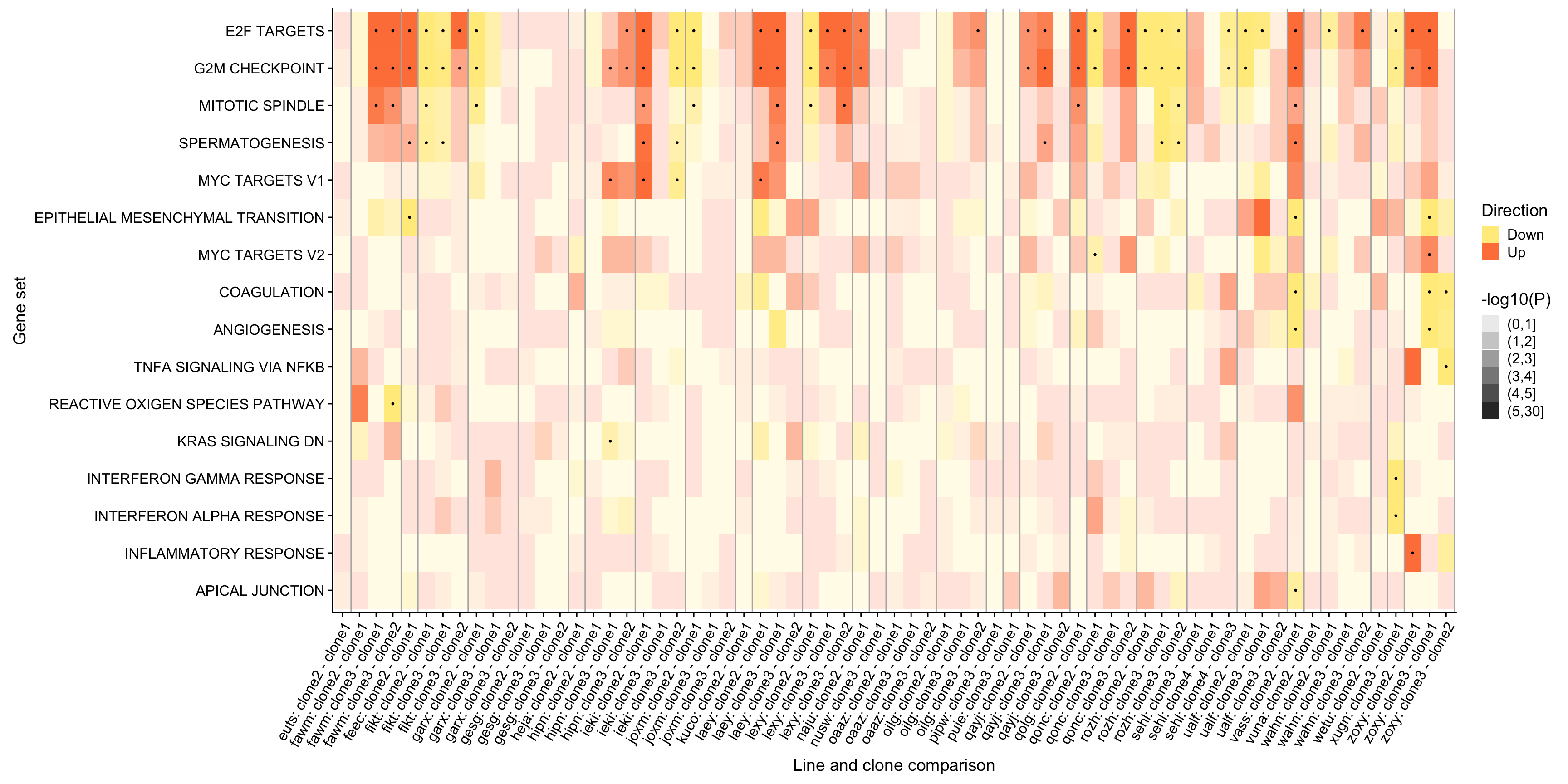

Expand here to see past versions of top_genesets_H_direction_heatmap_all_contrasts-1.png:

Version	Author	Date
02a8343	davismcc	2018-08-24
d2e8b31	davismcc	2018-08-19

ggsave("figures/differential_expression/top_genesets_H_direction_heatmap_all_contrasts.png", height = 9, width = 20)
ggsave("figures/differential_expression/top_genesets_H_direction_heatmap_all_contrasts.pdf", height = 9, width = 20)
ggsave("figures/differential_expression/top_genesets_H_direction_heatmap_all_contrasts.svg", height = 9, width = 20)

We can also add a panel to this figure showing the number of donors in which each of these gene sets is significantly enriched.

## Hallmark geneset
pp_nsig <- df_camera_sig_unst %>% dplyr::filter(collection == "H") %>% 
    dplyr::filter(stat == "logFC") %>%
    group_by(geneset) %>% 
    dplyr::mutate(id = paste0(donor, geneset)) %>% distinct(id, .keep_all = TRUE) %>%
    dplyr::summarise(n_donors = n()) %>% dplyr::arrange(geneset, n_donors) %>% ungroup() %>%
    dplyr::mutate(geneset = gsub("_", " ", gsub("HALLMARK_", "", geneset))) %>%
    ggplot(aes(y = n_donors, x = reorder(geneset, n_donors, max))) +
    geom_hline(yintercept = 0, colour = "gray50") +
    geom_segment(aes(xend = reorder(geneset, n_donors, max), yend = 0),
                 colour = "gray50") +
    geom_point(size = 4, colour = "gray30", alpha = 1) +
    ggthemes::scale_colour_tableau() +
    coord_flip() +
    xlab("Gene set") + ylab("Number of lines significant") +
    theme(axis.title.y = element_blank(),
          axis.text.y = element_blank(),
          axis.ticks.y = element_blank(),
          axis.line.y = element_blank())

prow <- plot_grid(pp + theme(legend.position = "none"), 
                  pp_nsig, align = 'h', rel_widths = c(7, 1))
lgnd <- get_legend(pp)
plot_grid(prow, lgnd, rel_widths = c(3, .3))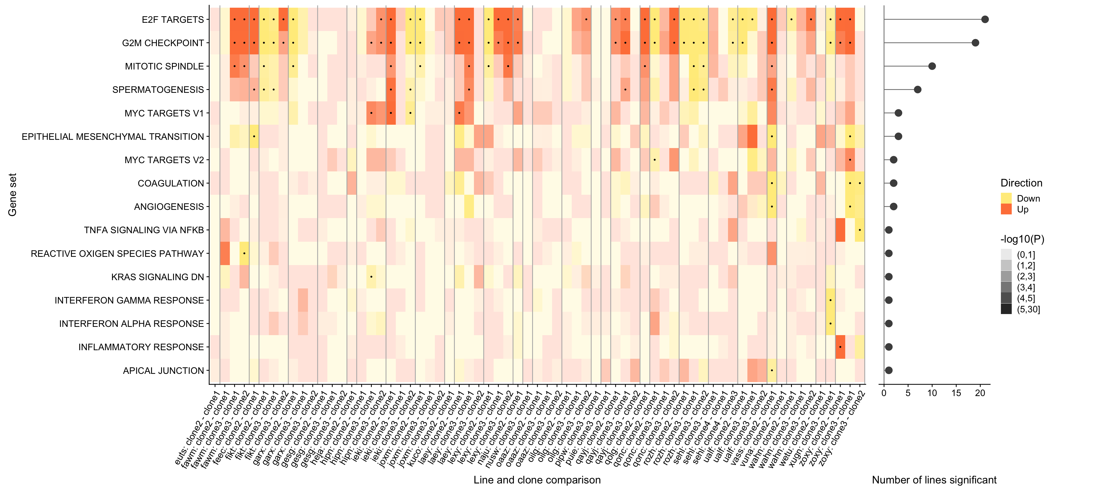

Expand here to see past versions of top_genesets_H_direction_heatmap_all_contrasts_with_nsig_donors-1.png:

Version	Author	Date
02a8343	davismcc	2018-08-24
d2e8b31	davismcc	2018-08-19

ggsave("figures/differential_expression/top_genesets_H_direction_heatmap_all_contrasts_with_nsig_donors.png", height = 9, width = 20)
ggsave("figures/differential_expression/top_genesets_H_direction_heatmap_all_contrasts_with_nsig_donors.pdf", height = 9, width = 20)
ggsave("figures/differential_expression/top_genesets_H_direction_heatmap_all_contrasts_with_nsig_donors.svg", height = 9, width = 20)

However, the plot above is very complicated, so we may want to focus just on the lines for which there are multiple clones that show differing behaviour amongst each other. To simplify, let us just look at 12 donors that have significant geneset enrichment for at least 2 contrasts and just look at the 9 gene sets that are significant in at least three lines.

repeated_sig_H_genesets3 <- df_camera_sig_unst %>% 
    dplyr::filter(collection == "H", stat == "logFC") %>% 
    group_by(geneset) %>% 
    dplyr::mutate(id = paste0(donor, geneset)) %>% distinct(id, .keep_all = TRUE) %>%
    dplyr::summarise(n_donors = n()) %>% dplyr::arrange(n_donors) %>% 
    dplyr::filter(n_donors > 2.5) 
repeated_sig_H_genesets_vec3 <- unique(repeated_sig_H_genesets3[["geneset"]])
repeated_sig_H_genesets_vec3 <- gsub("_", " ", gsub("HALLMARK_", "", 
                                                   repeated_sig_H_genesets_vec3))

selected_donors <- c("fawm", "fikt", "hipn", "ieki", "laey", "lexy", "qayj", 
                     "qonc", "rozh", "ualf", "wahn", "zoxy")

df_4_heatmap_filt <- df_camera_all_unst %>% 
  dplyr::mutate(geneset = gsub("_", " ", gsub("HALLMARK_", "", geneset))) %>%
  dplyr::mutate(geneset = 
                  factor(geneset, levels = repeated_sig_H_genesets_vec3)) %>%
  dplyr::filter(geneset %in% repeated_sig_H_genesets_vec3,
                donor %in% selected_donors) %>%
  dplyr::mutate(id = paste0(donor, ": ", contrast))

df_4_heatmap_filt_sig <- df_camera_sig_unst %>% 
  dplyr::filter(collection == "H", stat == "logFC") %>%
  dplyr::mutate(geneset = gsub("_", " ", gsub("HALLMARK_", "", geneset))) %>%
  dplyr::mutate(geneset = 
                  factor(geneset, levels = repeated_sig_H_genesets_vec3)) %>%
  dplyr::filter(geneset %in% repeated_sig_H_genesets_vec3,
                donor %in% selected_donors) %>%
  dplyr::mutate(id = paste0(donor, ": ", contrast))

df_4_heatmap_filt <- dplyr::mutate(
    df_4_heatmap_filt,
    minlog10P = cut(-log10(PValue), breaks = c(0, 1, 2, 3, 4, 5, 30)))

div_lines_filt <- gsub(": c.*", "",
                       sort(unique(paste0(df_4_heatmap_filt[["donor"]], ": ", 
                                          df_4_heatmap_filt[["contrast"]])))) %>% 
  table %>% cumsum + 0.5

pp_filt <- df_4_heatmap_filt %>%
    ggplot(aes(x = id, y = geneset, fill = Direction, alpha = minlog10P)) +
    geom_tile() +
    geom_point(alpha = 1, data = df_4_heatmap_filt_sig, pch = 19, size = 0.5, 
               show.legend = FALSE) +
    geom_vline(xintercept = div_lines_filt, colour = "gray70") +
    scale_fill_manual(values = c("lightgoldenrod1", "sienna1")) +
    scale_alpha_discrete(name = "-log10(P)") +
    ylab("Gene set") +
    xlab("Line and clone comparison") +
    theme(axis.text.x = element_text(angle = 60, hjust = 1),
          legend.position = "right")
pp_filt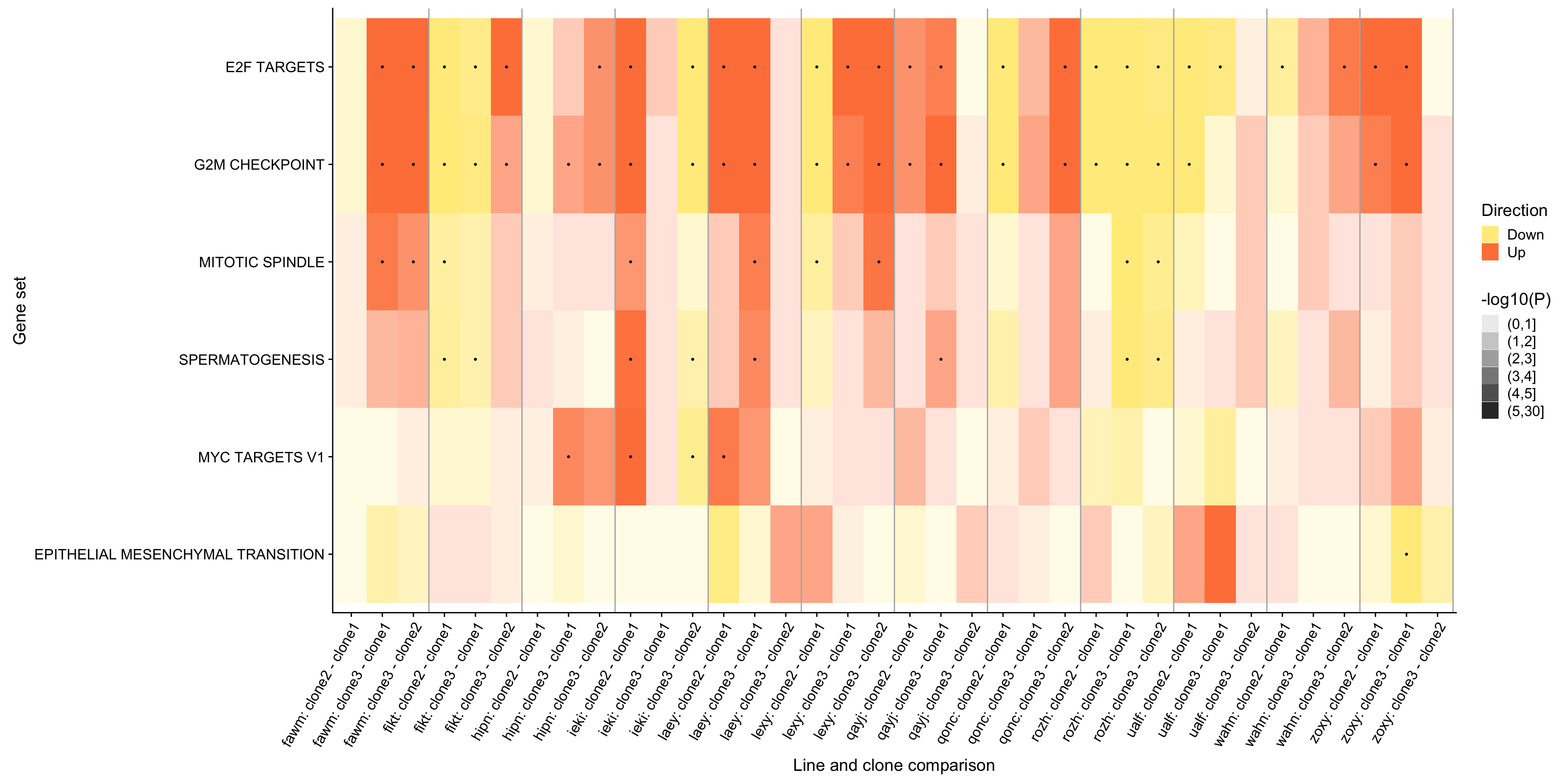

Expand here to see past versions of top_genesets_H_direction_heatmap_all_contrasts-simple-1.png:

Version	Author	Date
02a8343	davismcc	2018-08-24

ggsave("figures/differential_expression/top_genesets_H_direction_heatmap_filt_contrasts.png", plot = pp_filt, height = 5, width = 12)
ggsave("figures/differential_expression/top_genesets_H_direction_heatmap_filt_contrasts.pdf", plot = pp_filt, height = 5, width = 12)
ggsave("figures/differential_expression/top_genesets_H_direction_heatmap_filt_contrasts.svg", plot = pp_filt, height = 5, width = 12)

ggsave("figures/differential_expression/top_genesets_H_direction_heatmap_filt_contrasts_wide.png", plot = pp_filt, height = 5, width = 16)
ggsave("figures/differential_expression/top_genesets_H_direction_heatmap_filt_contrasts_wide.pdf", plot = pp_filt, height = 5, width = 16)
ggsave("figures/differential_expression/top_genesets_H_direction_heatmap_filt_contrasts_wide.svg", plot = pp_filt, height = 5, width = 16)

Correlation of gene set results and genes contained

Let’s look at the correlation between gene set results (Spearman correlation of signed -log10(P-values) from camera tests) and compare to the proportion of genes overlapping between pairs of gene sets.

repeated_sig_H_genesets_vec2 <- paste0("HALLMARK_", 
                                       gsub(" ", "_", repeated_sig_H_genesets_vec))
## all results
df_H_pvals <- df_camera_all_unst %>% dplyr::filter(collection == "H") %>% 
  dplyr::filter(stat == "logFC", geneset %in% repeated_sig_H_genesets_vec2) %>%
  dplyr::mutate(donor_coeff = paste(donor, coeff, sep = "."),
                sign = ifelse(Direction == "Down", -1, 1),
                signed_P = sign * -log10(PValue)) %>%
  dplyr::select(geneset, donor_coeff, signed_P) %>%
  tidyr::spread(key = donor_coeff, value = signed_P)

mat_H_pvals <- as.matrix(df_H_pvals[, -1])
rownames(mat_H_pvals) <- gsub("_", " ", gsub("HALLMARK_", "", df_H_pvals[[1]]))
cor_H_pvals <- cor(t(mat_H_pvals), method = "spearman")
p.mat <- cor_pmat(t(mat_H_pvals))
ggcorrplot(cor_H_pvals, hc.order = TRUE, p.mat = p.mat, insig = "blank") +
  theme(panel.grid.major = element_blank(),
        panel.grid.minor = element_blank())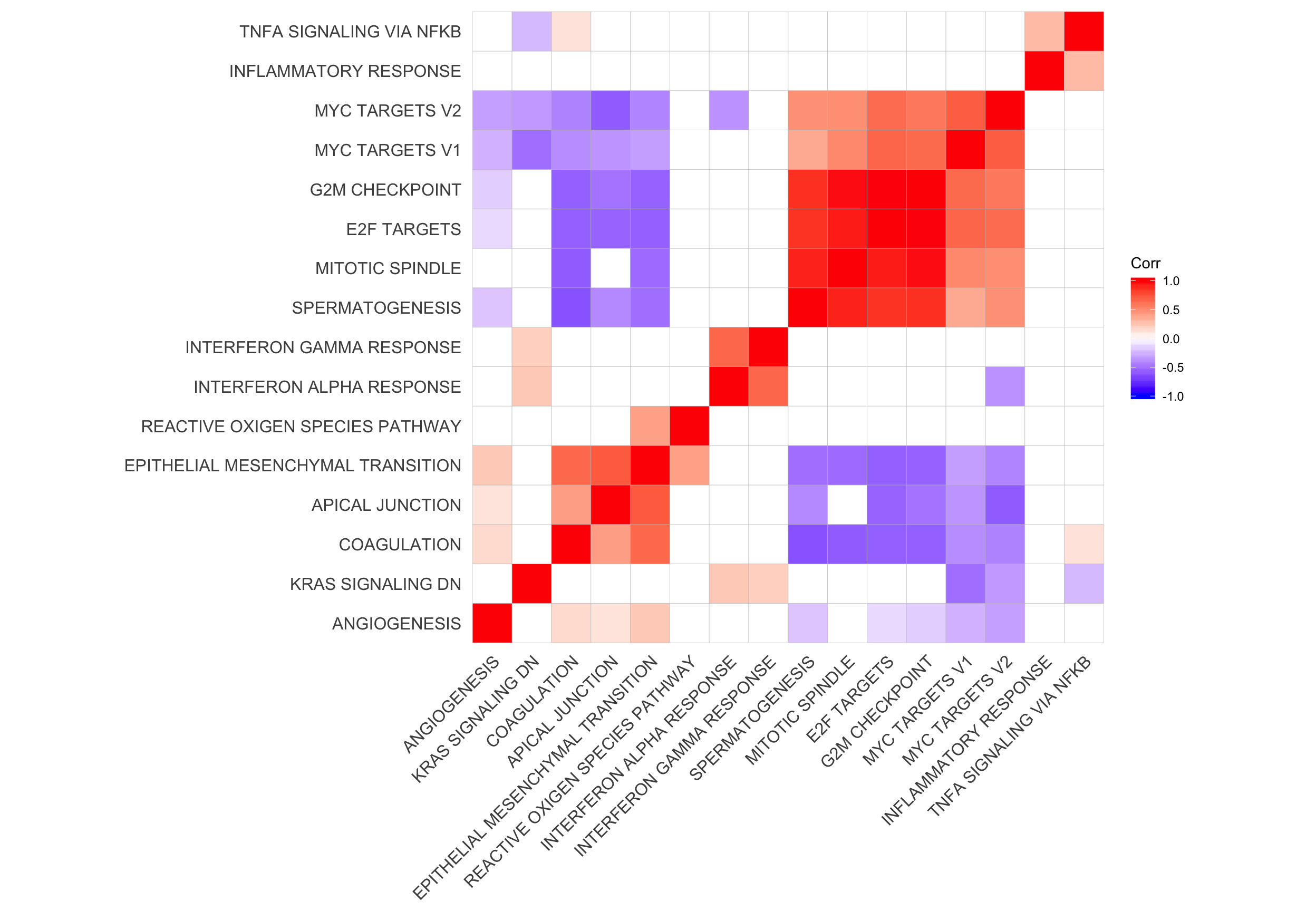

Expand here to see past versions of corr-maps-1.png:

Version	Author	Date
d2e8b31	davismcc	2018-08-19

hclust_cor <- hclust(as.dist(1 - cor_H_pvals))
corrplot1 <- ggcorrplot(cor_H_pvals[hclust_cor$order, hclust_cor$order], 
           p.mat = p.mat[hclust_cor$order, hclust_cor$order], insig = "blank") +
  theme(panel.grid.major = element_blank(),
        panel.grid.minor = element_blank())

mat_H_gene_overlap <- matrix(nrow = nrow(cor_H_pvals), ncol = ncol(cor_H_pvals),
                             dimnames = dimnames(cor_H_pvals))
for (i in seq_along(repeated_sig_H_genesets_vec2)) {
  for (j in seq_along(repeated_sig_H_genesets_vec2)) {
    gs1 <- paste0("HALLMARK_", gsub(" ", "_", rownames(mat_H_gene_overlap)[i]))
    gs2 <- paste0("HALLMARK_", gsub(" ", "_", rownames(mat_H_gene_overlap)[j]))
    mat_H_gene_overlap[i, j] <- mean(Hs.H[[gs1]] %in% Hs.H[[gs2]])
  }
}

corrplot2 <- ggcorrplot(mat_H_gene_overlap[hclust_cor$order, hclust_cor$order]) +
  scale_fill_gradient(name = "Gene set\noverlap", low = "white", high = "black") +
  theme(panel.grid.major = element_blank(),
        panel.grid.minor = element_blank())
corrplot2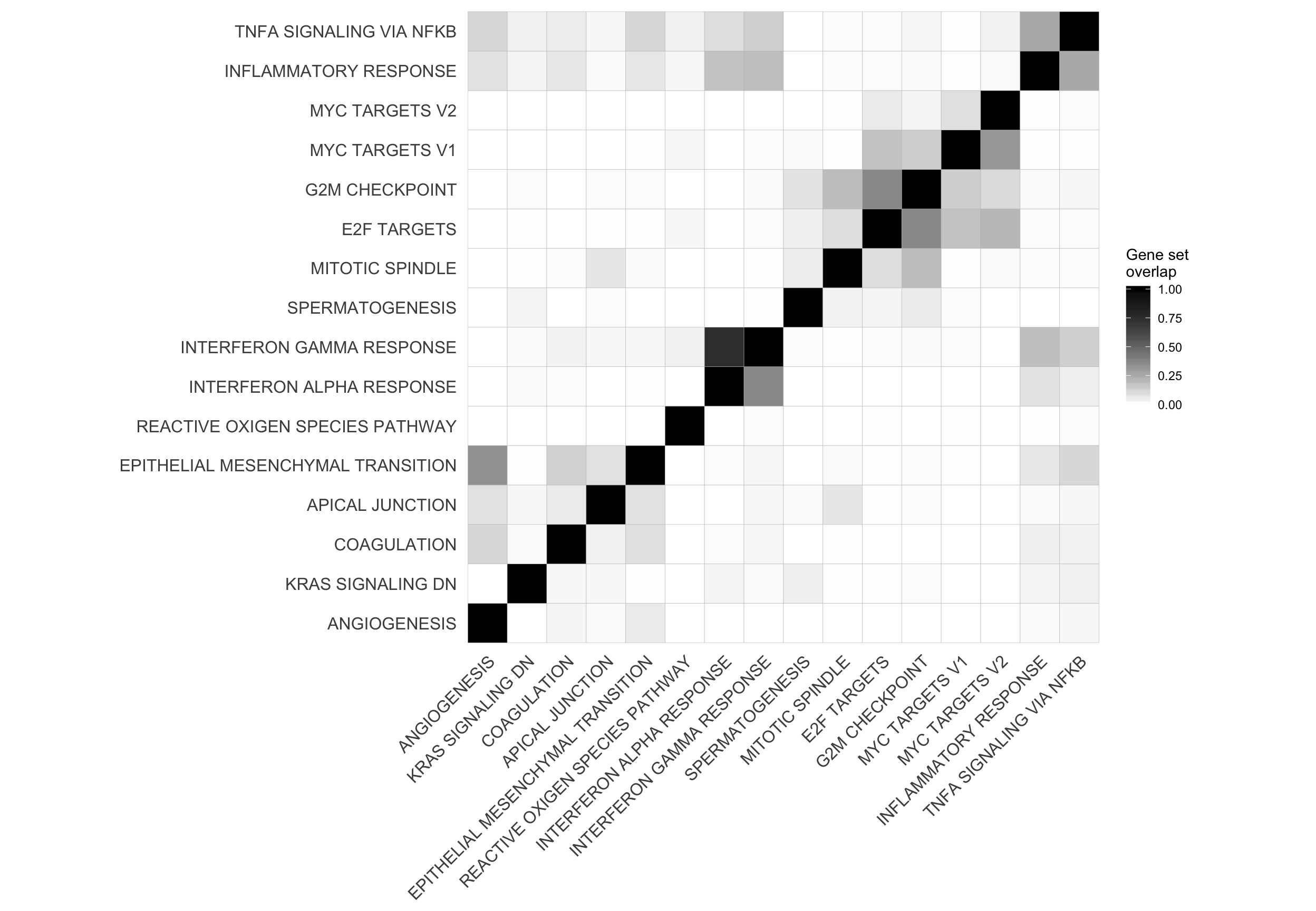

Expand here to see past versions of corr-maps-2.png:

Version	Author	Date
d2e8b31	davismcc	2018-08-19

corrplot3 <- corrplot2 + theme(axis.text.y = element_blank())

plot_grid(corrplot1 + theme(plot.margin = unit(c(0,0,0,0), "cm")), 
          corrplot3 + theme(plot.margin = unit(c(0,0,0,0), "cm")), 
          align = "h", axis = "b", rel_widths = c(0.58, 0.42))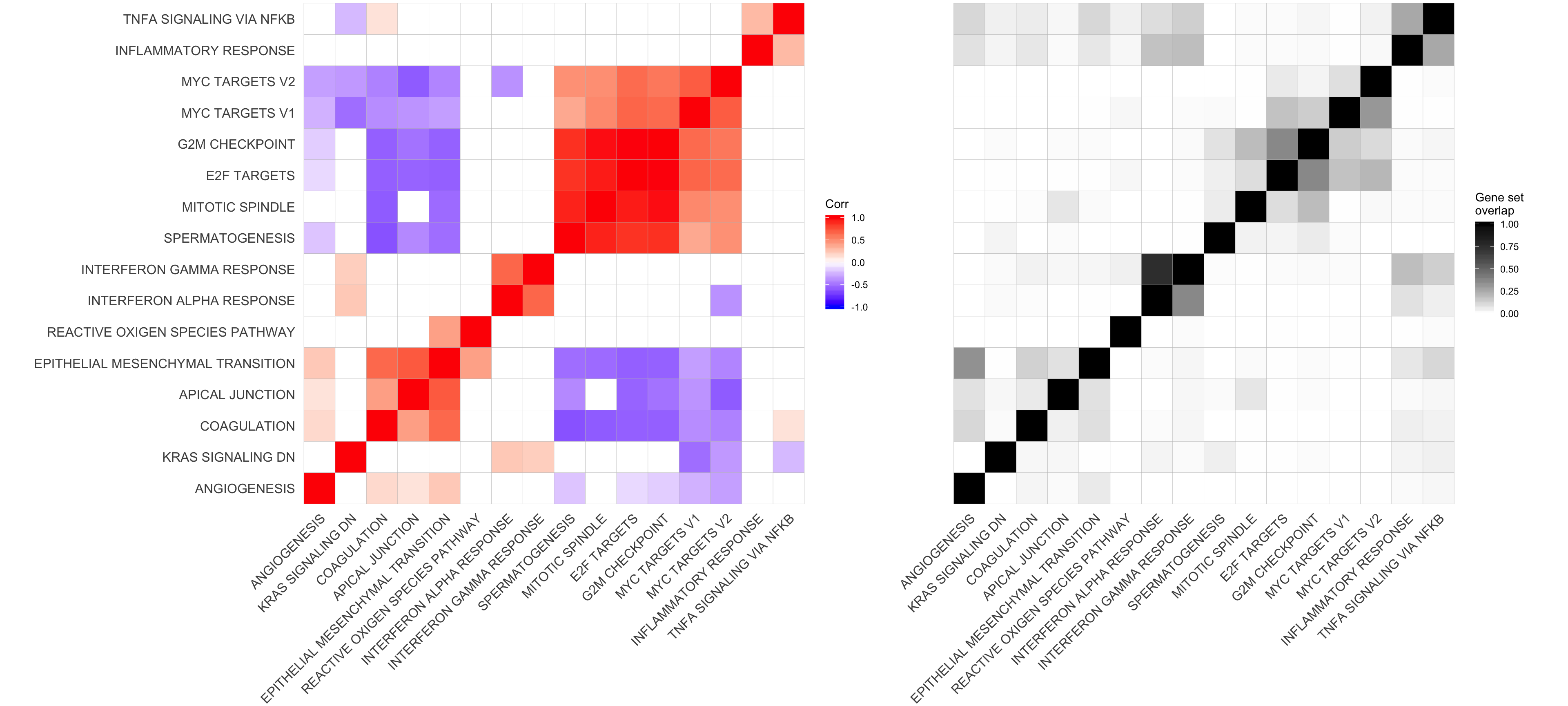

Expand here to see past versions of corr-plot-combined-1.png:

Version	Author	Date
d2e8b31	davismcc	2018-08-19

ggsave("figures/differential_expression/top_genesets_H_corrplots.png", height = 9, width = 20)
ggsave("figures/differential_expression/top_genesets_H_corrplots.pdf", height = 9, width = 20)
ggsave("figures/differential_expression/top_genesets_H_corrplots.svg", height = 9, width = 20)

Plot gene set correlation with the number of donors in which each gene set is significant.

pp_nsig <- df_camera_sig_unst %>% dplyr::filter(collection == "H") %>% 
    dplyr::filter(stat == "logFC") %>%
    group_by(geneset) %>% 
    dplyr::mutate(id = paste0(donor, geneset)) %>% distinct(id, .keep_all = TRUE) %>%
    dplyr::summarise(n_donors = n()) %>% dplyr::arrange(geneset, n_donors) %>% ungroup() %>%
    dplyr::mutate(geneset = gsub("_", " ", gsub("HALLMARK_", "", geneset))) %>%
    dplyr::mutate(geneset = factor(
      geneset, levels = rownames(mat_H_gene_overlap)[hclust_cor$order])) %>%
    ggplot(aes(y = n_donors, x = geneset)) +
    geom_hline(yintercept = 0, colour = "gray50") +
    geom_segment(aes(xend = geneset, yend = 0),
                 colour = "gray50") +
    geom_point(size = 4, colour = "gray30", alpha = 1) +
    ggthemes::scale_colour_tableau() +
    coord_flip() +
    xlab("Gene set") + ylab("Number of lines\nsignificant") +
    theme(axis.title.y = element_blank(),
          axis.text.y = element_blank(),
          axis.ticks.y = element_blank(),
          axis.line.y = element_blank())

ggdraw() +
  draw_plot(corrplot1 + theme(legend.position = "top"), 
            x = 0,  y = 0, width = 0.8, scale = 1) +
  draw_plot(pp_nsig, 
            x = 0.685,  y = 0.25, width = 0.25, height = 0.6445)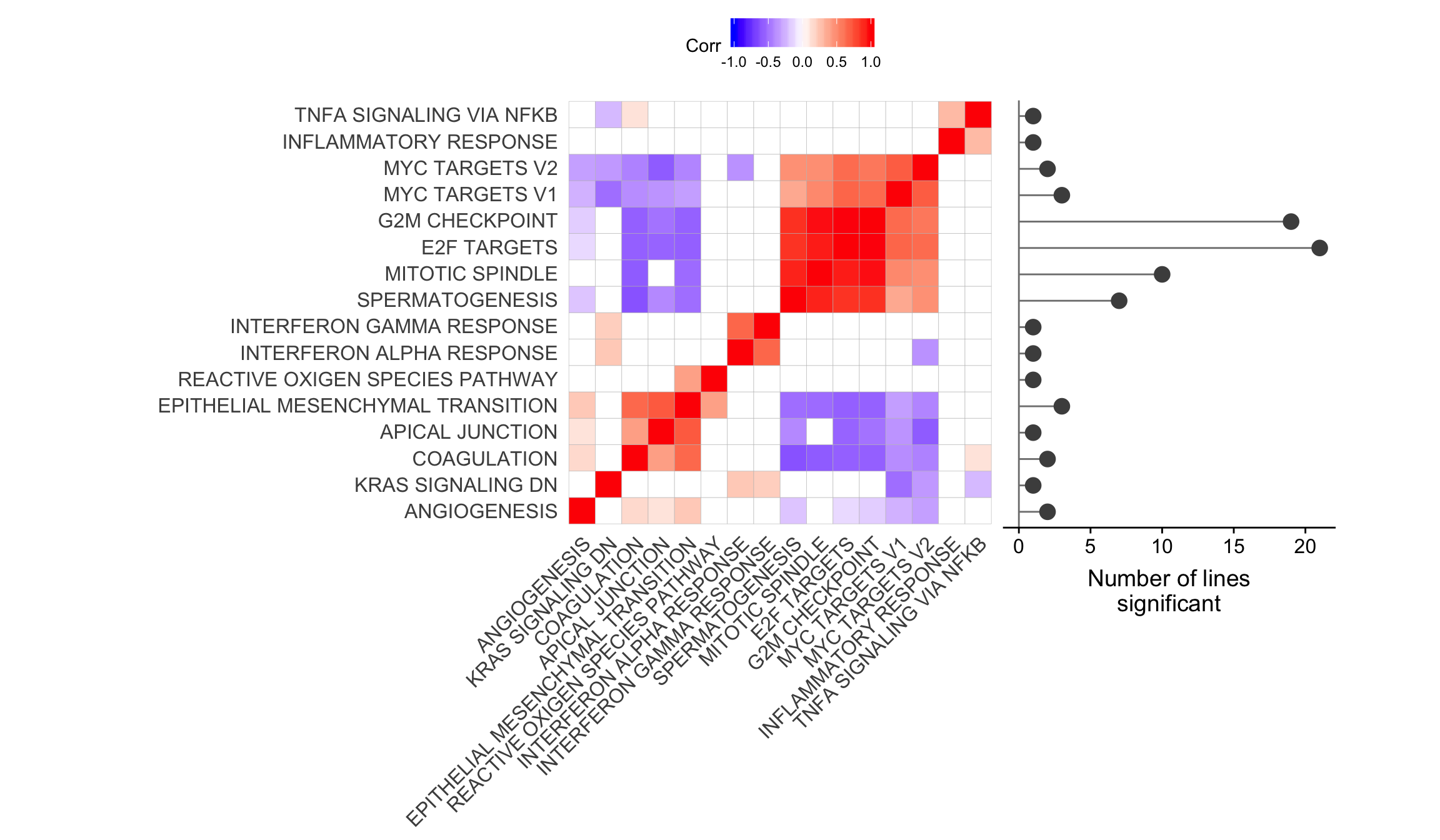

Expand here to see past versions of unnamed-chunk-4-1.png:

Version	Author	Date
02a8343	davismcc	2018-08-24
d2e8b31	davismcc	2018-08-19

ggsave("figures/differential_expression/top_genesets_H_corrplot_with_nsig_donor.png", 
       height = 7, width = 12)
ggsave("figures/differential_expression/top_genesets_H_corrplot_with_nsig_donor.pdf", 
       height = 7, width = 12)

Linking DE to selection

df_donor_info <- read.table("data/donor_info_070818.txt")
df_donor_info <- as_data_frame(df_donor_info)
df_donor_info$donor <- df_donor_info$donor_short

df_ncells_de <- assignments %>% dplyr::filter(assigned != "unassigned", 
                              donor_short_id %in% names(de_res$qlf_list)) %>%
    group_by(donor_short_id) %>%
    dplyr::summarise(n_cells = n())
colnames(df_ncells_de)[1] <- "donor"

df_prop_assigned <- assignments %>% 
  dplyr::filter(donor_short_id %in% names(de_res$qlf_list)) %>%
    group_by(donor_short_id) %>%
    dplyr::summarise(prop_assigned = mean(assigned != "unassigned"))
colnames(df_prop_assigned)[1] <- "donor"

df_nvars_by_cat <- readr::read_tsv("output/nvars_by_category_by_donor.tsv")
df_nvars_by_cat_wd <- tidyr::spread(
  df_nvars_by_cat[, 1:3], consequence, n_vars_all_genes)
df_nvars_by_cat_wd <- left_join(
  dplyr::summarise(group_by(df_nvars_by_cat, donor), nvars_all = sum(n_vars_all_genes)),
  df_nvars_by_cat_wd
)
df_nvars_by_cat_wd <- df_nvars_by_cat %>% 
  dplyr::filter(consequence %in% c("missense", "splicing", "nonsense")) %>%
  group_by(donor) %>%
  dplyr::summarise(nvars_misnonspli = sum(n_vars_all_genes)) %>%
  left_join(., df_nvars_by_cat_wd)

df_donor_info <- left_join(df_ncells_de, df_donor_info)
df_donor_info <- left_join(df_prop_assigned, df_donor_info)
df_donor_info <- left_join(df_donor_n_de, df_donor_info)
df_donor_info$n_de_genes <- df_donor_info$count
df_donor_info <- left_join(df_donor_info, df_nvars_by_cat_wd)

nbglm_nde <- MASS::glm.nb(n_de_genes ~ n_cells, data = df_donor_info)
df_nbglm_nde <- broom::augment(nbglm_nde) %>%
  left_join(df_donor_info)

## n_de vs n_cells
df_nbglm_nde %>%
  dplyr::mutate(selection = factor(
    selection, levels = c("neutral", "undetermined", "selected"))) %>%
ggplot(aes(x = n_cells, y = n_de_genes, fill = selection)) +
  geom_smooth(aes(group = 1), colour = "firebrick", method = "lm", level = 0.9) +
  geom_point(size = 3, shape = 21) +
  ylab("Number of DE genes") +
  xlab("Number of cells") +
  scale_fill_manual(values = c("dodgerblue", "#CCCCCC", "dodgerblue4"))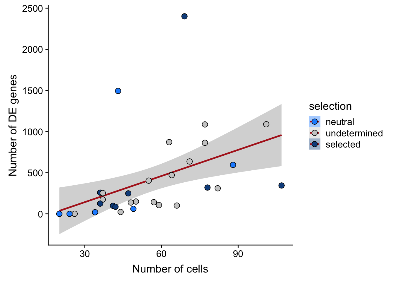

Expand here to see past versions of link-de-to-selection-1.png:

Version	Author	Date
a056169	davismcc	2018-08-27

ggsave("figures/differential_expression/n_de_genes_vs_n_cells.png", 
       height = 5.5, width = 5.5)

## selection, n_de resid boxplot
df_nbglm_nde %>%
  dplyr::mutate(selection = factor(
    selection, levels = c("neutral", "undetermined", "selected"))) %>%
ggplot(aes(x = selection, y = .resid)) +
  geom_violin(aes(fill = selection), alpha = 0.7) +
  geom_boxplot(outlier.alpha = 0, width = 0.2) +
  ggbeeswarm::geom_quasirandom(aes(fill = selection), size = 3, shape = 21) +
  ylab("Number of DE genes (residual from NB GLM)") +
  xlab("Inferred selection status") +
  scale_fill_manual(values = c("dodgerblue", "#CCCCCC", "dodgerblue4")) +
  coord_flip()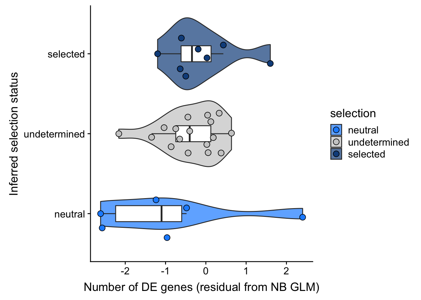

Expand here to see past versions of link-de-to-selection-2.png:

Version	Author	Date
a056169	davismcc	2018-08-27

ggsave("figures/differential_expression/n_de_resid_selection_boxplot.png", 
       height = 4.5, width = 6.5)

summary(lm(.resid ~ selection, data = df_nbglm_nde))


Call:
lm(formula = .resid ~ selection, data = df_nbglm_nde)

Residuals:
    Min      1Q  Median      3Q     Max 
-1.7896 -0.4823 -0.0568  0.4630  3.3122 

Coefficients:
                      Estimate Std. Error t value Pr(>|t|)  
(Intercept)            -0.9100     0.4242  -2.145   0.0408 *
selectionselected       0.7766     0.5612   1.384   0.1773  
selectionundetermined   0.5391     0.4934   1.093   0.2839  
---
Signif. codes:  0 '***' 0.001 '**' 0.01 '*' 0.05 '.' 0.1 ' ' 1

Residual standard error: 1.039 on 28 degrees of freedom
Multiple R-squared:  0.06604,   Adjusted R-squared:  -0.0006725 
F-statistic: 0.9899 on 2 and 28 DF,  p-value: 0.3842

## selection, n_de (sqrt scale) boxplot
df_nbglm_nde %>%
  dplyr::mutate(selection = factor(
    selection, levels = c("neutral", "undetermined", "selected"))) %>%
ggplot(aes(x = selection, y = n_de_genes)) +
  geom_violin(aes(fill = selection), alpha = 0.7) +
  geom_boxplot(outlier.alpha = 0, width = 0.2) +
  ggbeeswarm::geom_quasirandom(aes(fill = selection), size = 3, shape = 21) +
  ylab("Number of DE genes") +
  xlab("Inferred selection status") +
  scale_y_sqrt(breaks = c(0, 100, 500, 1000, 1500, 2000, 2500)) +
  scale_fill_manual(values = c("dodgerblue", "#CCCCCC", "dodgerblue4")) +
  coord_flip()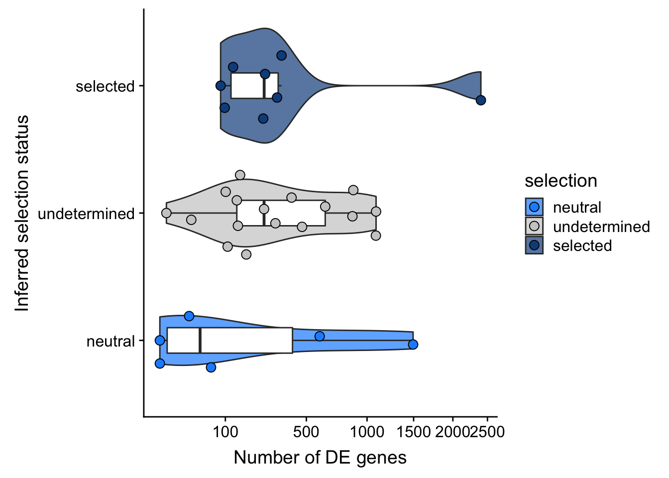

Expand here to see past versions of link-de-to-selection-3.png:

Version	Author	Date
a056169	davismcc	2018-08-27

ggsave("figures/differential_expression/n_de_sqrt_selection_boxplot.png", 
       height = 5.5, width = 6.5)

## n_de (resids) vs goodness of fit cumul. mutation model
df_nbglm_nde %>%
  dplyr::mutate(selection = factor(
    selection, levels = c("neutral", "undetermined", "selected"))) %>%
ggplot(aes(x = rsq_ntrtestr, y = .resid, fill = selection)) +
  geom_smooth(aes(group = 1), colour = "firebrick", method = "lm", level = 0.9) +
  geom_point(size = 3, shape = 21) +
  ylab("Number of DE genes (residual from NB GLM)") +
  xlab("Goodness of fit: cumulative mutations") +
  scale_fill_manual(values = c("dodgerblue", "#CCCCCC", "dodgerblue4"))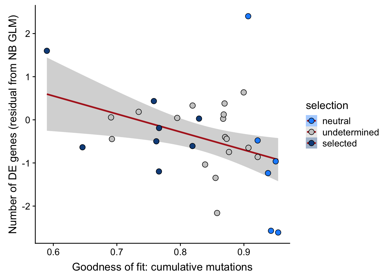

Expand here to see past versions of link-de-to-selection-4.png:

Version	Author	Date
a056169	davismcc	2018-08-27

ggsave("figures/differential_expression/n_de_resid_selection_vs_gof_cumul_mut_model.png", 
       height = 6.5, width = 5.5)


## n_de (sqrt scale) vs goodness of fit cumul. mutation model
df_nbglm_nde %>%
  dplyr::mutate(selection = factor(
    selection, levels = c("neutral", "undetermined", "selected"))) %>%
ggplot(aes(x = rsq_ntrtestr, y = n_de_genes, fill = selection)) +
  geom_smooth(aes(group = 1), colour = "firebrick", method = "lm", level = 0.9) +
  geom_point(size = 3, shape = 21) +
  ylab("Number of DE genes") +
  xlab("Goodness of fit: cumulative mutations") +
  scale_fill_manual(values = c("dodgerblue", "#CCCCCC", "dodgerblue4"))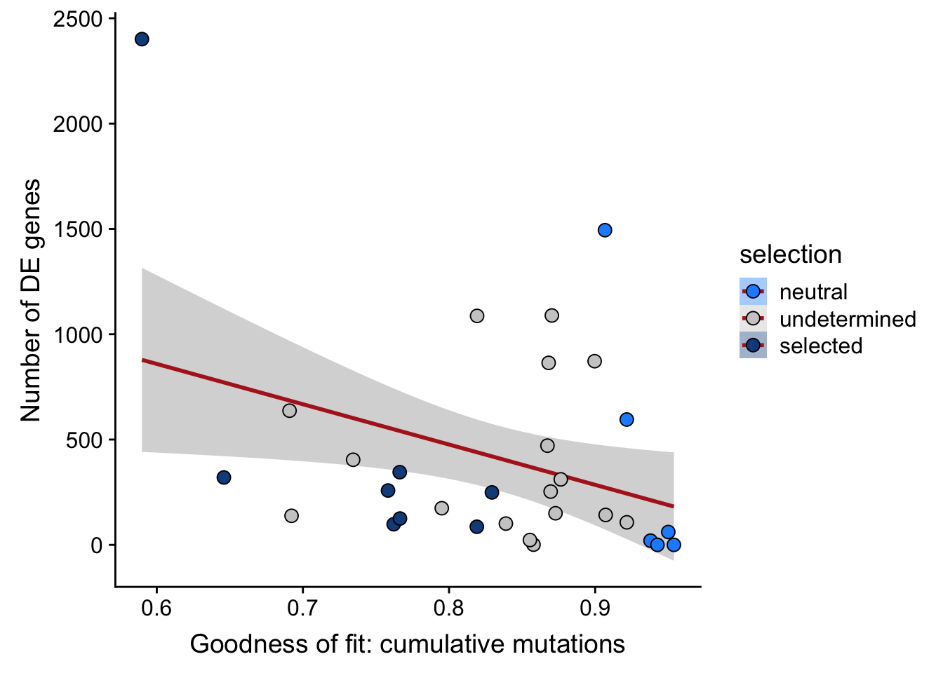

Expand here to see past versions of link-de-to-selection-5.png:

Version	Author	Date
a056169	davismcc	2018-08-27

ggsave("figures/differential_expression/n_de_sqrt_selection_vs_gof_cumul_mut_model.png", 
       height = 5.5, width = 6.5)

## n_de (resids) vs goodness of fit NB model
df_nbglm_nde %>%
  dplyr::mutate(selection = factor(
    selection, levels = c("neutral", "undetermined", "selected"))) %>%
ggplot(aes(x = rsq_negbinfit, y = .resid, fill = selection)) +
  geom_smooth(aes(group = 1), colour = "firebrick", method = "lm", level = 0.9) +
  geom_point(size = 3, shape = 21) +
  ylab("Number of DE genes (residual from NB GLM)") +
  xlab("Goodness of fit: negative binomial distribution") +
  scale_fill_manual(values = c("dodgerblue", "#CCCCCC", "dodgerblue4"))

Expand here to see past versions of link-de-to-selection-6.png:

Version	Author	Date
a056169	davismcc	2018-08-27

ggsave("figures/differential_expression/n_de_resid_selection_vs_gof_negbin_model.png", 
       height = 5.5, width = 6.5)

## n_de (resids) vs ave goodness of fit from both models
df_nbglm_nde %>%
  dplyr::mutate(selection = factor(
    selection, levels = c("neutral", "undetermined", "selected"))) %>%
ggplot(aes(x = (rsq_negbinfit + rsq_ntrtestr) / 2, y = .resid, fill = selection)) +
  geom_smooth(aes(group = 1), colour = "firebrick", method = "lm", level = 0.9) +
  geom_point(size = 3, shape = 21) +
  ylab("Number of DE genes (residual from NB GLM)") +
  xlab("Ave. goodness of fit:\n negative binomial & cumulative mutations") +
  scale_fill_manual(values = c("dodgerblue", "#CCCCCC", "dodgerblue4"))

Expand here to see past versions of link-de-to-selection-7.png:

Version	Author	Date
f0ed980	davismcc	2018-08-31
a056169	davismcc	2018-08-27

ggsave("figures/differential_expression/n_de_resid_selection_vs_ave_gof_2_models.png", 
       height = 5.5, width = 6.5)

## n_de vs ave goodness of fit from both models
df_nbglm_nde %>%
  dplyr::mutate(selection = factor(
    selection, levels = c("neutral", "undetermined", "selected"))) %>%
ggplot(aes(x = (rsq_negbinfit + rsq_ntrtestr) / 2, y = n_de_genes, 
           fill = selection)) +
  geom_smooth(aes(group = 1), colour = "firebrick", method = "lm", level = 0.9) +
  geom_point(size = 3, shape = 21) +
  scale_y_sqrt() +
  ylab("Number of DE genes") +
  xlab("Ave. goodness of fit:\n negative binomial & cumulative mutations") +
  scale_fill_manual(values = c("dodgerblue", "#CCCCCC", "dodgerblue4"))

Expand here to see past versions of link-de-to-selection-8.png:

Version	Author	Date
f0ed980	davismcc	2018-08-31
a056169	davismcc	2018-08-27

## n_de (resids) vs mutational load (all)
df_nbglm_nde %>%
  dplyr::mutate(selection = factor(
    selection, levels = c("neutral", "undetermined", "selected"))) %>%
ggplot(aes(x = nvars_all, y = .resid, fill = selection)) +
  geom_smooth(aes(group = 1), colour = "firebrick", method = "lm", level = 0.9) +
  geom_point(size = 3, shape = 21) +
  ylab("Number of DE genes (residual from NB GLM)") +
  xlab("Number of somatic variants") +
  scale_fill_manual(values = c("dodgerblue", "#CCCCCC", "dodgerblue4")) +
  scale_x_log10(breaks = c(5, 10, 20, 50, 100, 500))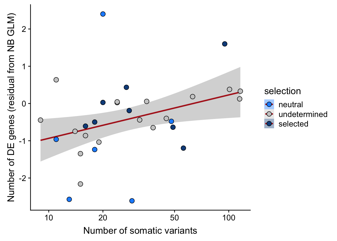

Expand here to see past versions of link-de-to-selection-9.png:

Version	Author	Date
f0ed980	davismcc	2018-08-31
a056169	davismcc	2018-08-27

ggsave("figures/differential_expression/n_de_resid_selection_vs_n_somatic_vars_all.png", 
       height = 6.5, width = 5.5)

## n_de (sqrt scale) vs mutational load (all)
df_nbglm_nde %>%
  dplyr::mutate(selection = factor(
    selection, levels = c("neutral", "undetermined", "selected"))) %>%
ggplot(aes(x = nvars_all, y = n_de_genes, fill = selection)) +
  geom_smooth(aes(group = 1), colour = "firebrick", method = "lm", level = 0.9) +
  geom_point(size = 3, shape = 21) +
  ylab("Number of DE genes") +
  xlab("Number of somatic variants") +
  scale_fill_manual(values = c("dodgerblue", "#CCCCCC", "dodgerblue4")) +
  scale_x_log10(breaks = c(5, 10, 20, 50, 100, 500)) +
  scale_y_sqrt(breaks = c(10, 100, 500, 1000, 1500, 2000, 2500))

Expand here to see past versions of link-de-to-selection-10.png:

Version	Author	Date
f0ed980	davismcc	2018-08-31
a056169	davismcc	2018-08-27

ggsave("figures/differential_expression/n_de_sqrt_selection_vs_n_somatic_vars_all.png", 
       height = 5.5, width = 6.5)

## n_de (resids) vs mutational load (missense)
df_nbglm_nde %>%
  dplyr::mutate(selection = factor(
    selection, levels = c("neutral", "undetermined", "selected"))) %>%
ggplot(aes(x = missense, y = .resid, fill = selection)) +
  geom_smooth(aes(group = 1), colour = "firebrick", method = "lm", level = 0.9) +
  geom_point(size = 3, shape = 21) +
  ylab("Number of DE genes (residual from NB GLM)") +
  xlab("Number of somatic missense variants") +
  scale_fill_manual(values = c("dodgerblue", "#CCCCCC", "dodgerblue4")) +
  scale_x_log10(breaks = c(5, 10, 20, 50, 100, 500))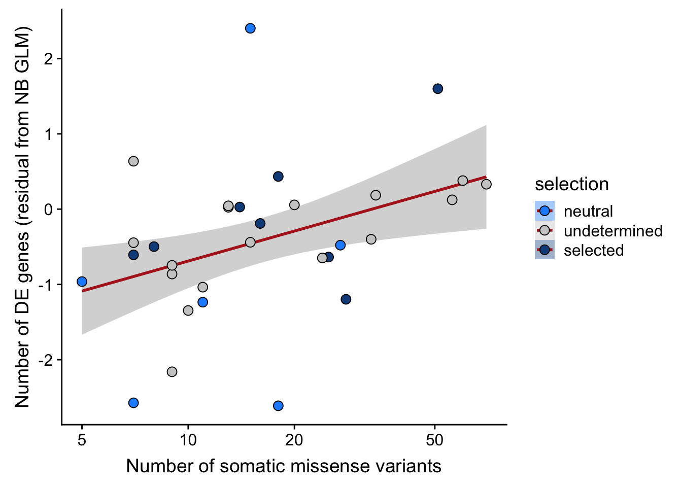

Expand here to see past versions of link-de-to-selection-11.png:

Version	Author	Date
f0ed980	davismcc	2018-08-31
a056169	davismcc	2018-08-27

ggsave("figures/differential_expression/n_de_resid_selection_vs_n_somatic_vars_missense.png", 
       height = 5.5, width = 6.5)

## n_de (resids) vs mutational load (missense, nonsense, splicing)
df_nbglm_nde %>%
  dplyr::mutate(selection = factor(
    selection, levels = c("neutral", "undetermined", "selected"))) %>%
ggplot(aes(x = nvars_misnonspli, y = .resid, fill = selection)) +
  geom_smooth(aes(group = 1), colour = "firebrick", method = "lm", level = 0.9) +
  geom_point(size = 3, shape = 21) +
  ylab("Number of DE genes (residual from NB GLM)") +
  xlab("Number of missense, nonsense & splicing variants") +
  scale_fill_manual(values = c("dodgerblue", "#CCCCCC", "dodgerblue4")) +
  scale_x_log10(breaks = c(5, 10, 20, 50, 100, 500))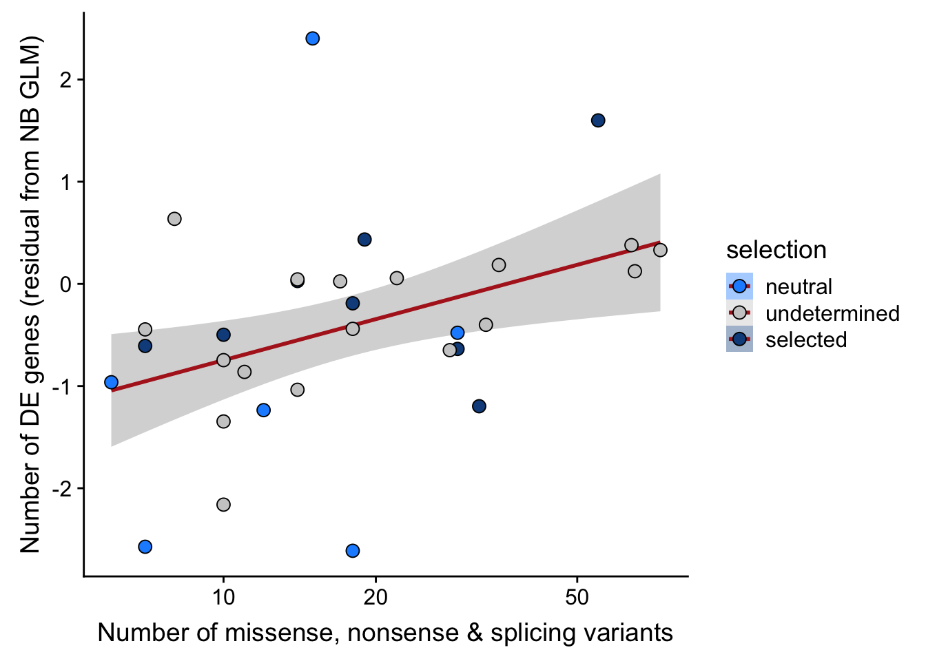

Expand here to see past versions of link-de-to-selection-12.png:

Version	Author	Date
f0ed980	davismcc	2018-08-31

ggsave("figures/differential_expression/n_de_resid_selection_vs_n_somatic_vars_misnonspli.png", 
       height = 6.5, width = 5.5)

df_nbglm_nde %>%
  dplyr::mutate(selection = factor(
    selection, levels = c("neutral", "undetermined", "selected"))) %>%
ggplot(aes(x = nvars_all, y = rsq_ntrtestr, fill = selection)) +
  geom_smooth(aes(group = 1), colour = "firebrick", method = "lm", level = 0.9) +
  geom_point(size = 3, shape = 21) +
  ylab("Goodness of fit: cumulative mutations ") +
  xlab("Number of somatic variants") +
  scale_fill_manual(values = c("dodgerblue", "#CCCCCC", "dodgerblue4")) +
  scale_x_log10(breaks = c(5, 10, 20, 50, 100, 500))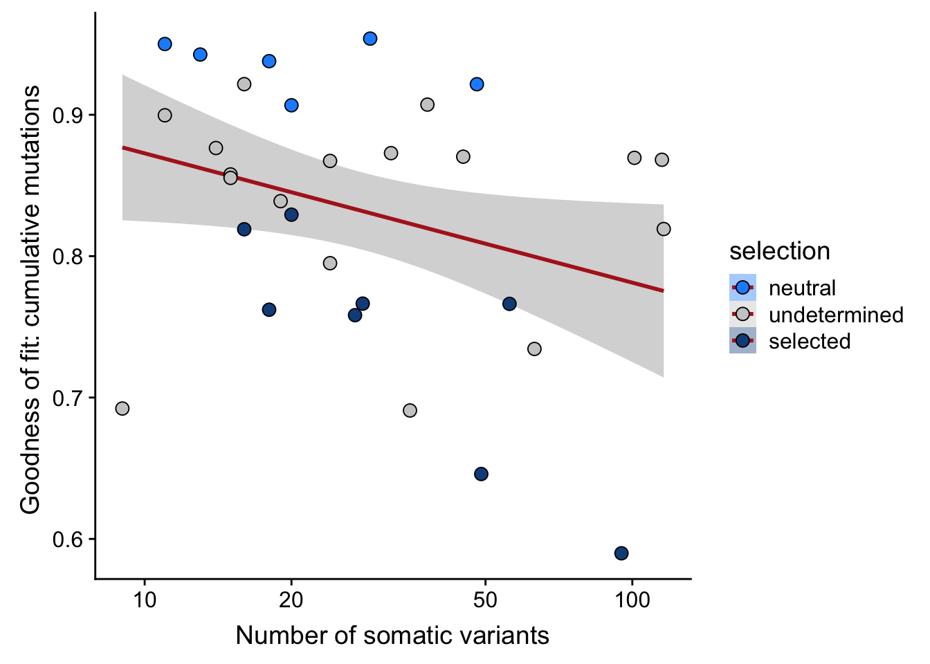

Expand here to see past versions of link-de-to-selection-13.png:

Version	Author	Date
f0ed980	davismcc	2018-08-31

ggsave("figures/differential_expression/gof_cumul_mut_model_vs_n_somatic_vars.png", 
       height = 6.5, width = 5.5)

We can also check the relationship between the number of somatic variants and evidence for selection as immediately above, but fliping the relationship.

df_nbglm_nde %>%
  dplyr::mutate(selection = factor(
    selection, levels = c("neutral", "undetermined", "selected"))) %>%
ggplot(aes(x = rsq_ntrtestr, y = nvars_all, fill = selection)) +
  geom_smooth(aes(group = 1), colour = "firebrick", method = "lm", level = 0.9) +
  geom_point(size = 3, shape = 21) +
  xlab("Goodness of fit: cumulative mutations ") +
  ylab(bquote("Number of somatic variants (log"[10]~ "scale)")) +
  scale_fill_manual(values = c("dodgerblue", "#CCCCCC", "dodgerblue4")) +
  scale_y_log10(breaks = c(5, 10, 20, 50, 100, 500))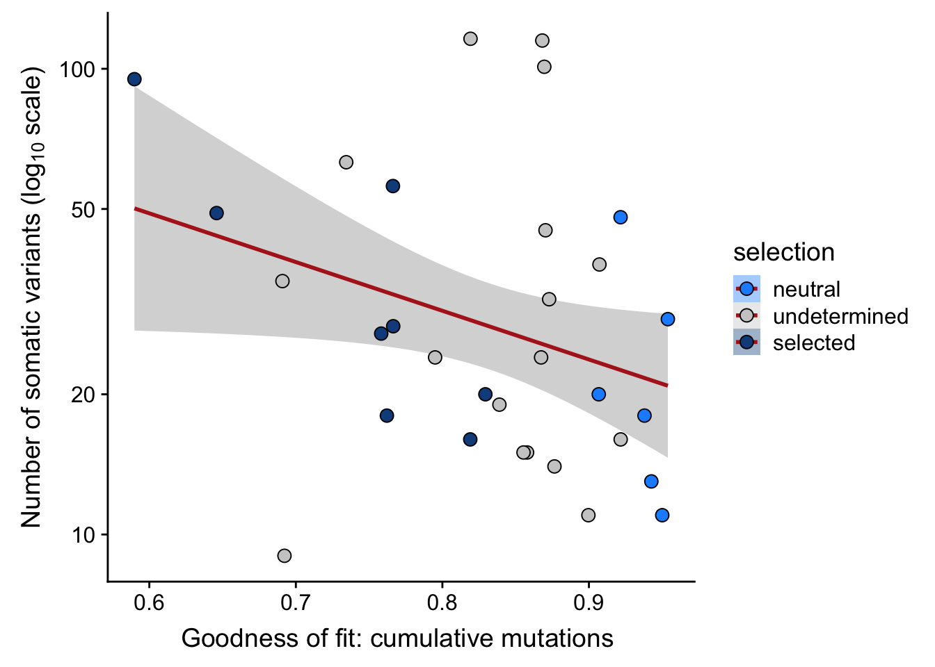

Expand here to see past versions of nvars-vs-gof-selection-1.png:

Version	Author	Date
f0ed980	davismcc	2018-08-31

ggsave("figures/differential_expression/n_somatic_vars_vs_gof_cumul_mut_model.png", 
       height = 6.5, width = 5.5)

df_nbglm_nde %>%
  dplyr::mutate(selection = factor(
    selection, levels = c("neutral", "undetermined", "selected"))) %>%
ggplot(aes(x = rsq_negbinfit, y = nvars_all, fill = selection)) +
  geom_smooth(aes(group = 1), colour = "firebrick", method = "lm", level = 0.9) +
  geom_point(size = 3, shape = 21) +
  xlab("Goodness of fit: negative binomial ") +
  ylab(bquote("Number of somatic variants (log"[10]~ "scale)")) +
  scale_fill_manual(values = c("dodgerblue", "#CCCCCC", "dodgerblue4")) +
  scale_y_log10(breaks = c(5, 10, 20, 50, 100, 500))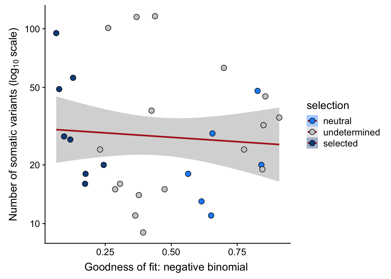

Expand here to see past versions of nvars-vs-gof-selection-2.png:

Version	Author	Date
f0ed980	davismcc	2018-08-31

ggsave("figures/differential_expression/n_somatic_vars_vs_gof_cumul_mut_model.png", 
       height = 6.5, width = 5.5)

df_nbglm_nde %>%
  dplyr::mutate(selection = factor(
    selection, levels = c("neutral", "undetermined", "selected"))) %>%
ggplot(aes(x = (rsq_negbinfit + rsq_ntrtestr) / 2, y = nvars_all, 
           fill = selection)) +
  geom_smooth(aes(group = 1), colour = "firebrick", method = "lm", level = 0.9) +
  geom_point(size = 3, shape = 21) +
  xlab("Ave. goodness of fit:\n negative binomial & cumulative mutations") +
  ylab(bquote("Number of somatic variants (log"[10]~ "scale)")) +
  scale_fill_manual(values = c("dodgerblue", "#CCCCCC", "dodgerblue4")) +
  scale_y_log10(breaks = c(5, 10, 20, 50, 100, 500))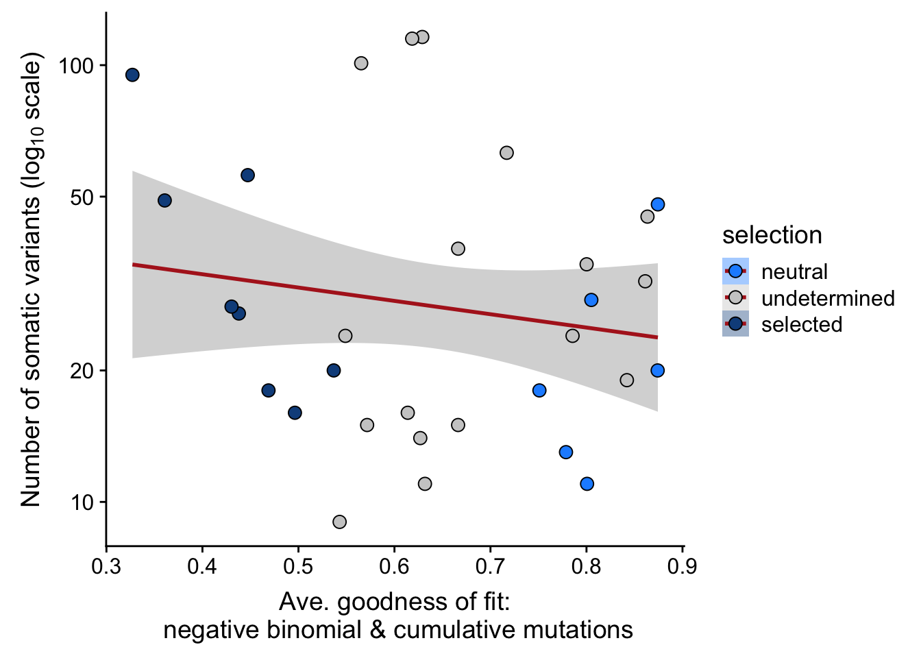

Expand here to see past versions of nvars-vs-gof-selection-3.png:

Version	Author	Date
f0ed980	davismcc	2018-08-31

ggsave("figures/differential_expression/n_somatic_vars_vs_ave_gof_two_models.png", 
       height = 6.5, width = 5.5)

p1 <- df_nbglm_nde %>%
  dplyr::mutate(selection = factor(
    selection, levels = c("neutral", "undetermined", "selected"))) %>%
ggplot(aes(x = rsq_ntrtestr, y = .resid, 
           fill = selection)) +
  geom_smooth(aes(group = 1), colour = "firebrick", method = "lm", level = 0.9) +
  geom_point(size = 3, shape = 21) +
  ylab("Number of DE genes (residual from NB GLM)") +
  xlab("Goodness of fit: cumulative mutations ") +
  scale_fill_manual(values = c("dodgerblue", "#CCCCCC", "dodgerblue4"))

p2 <- df_nbglm_nde %>%
  dplyr::mutate(selection = factor(
    selection, levels = c("neutral", "undetermined", "selected"))) %>%
ggplot(aes(x = nvars_all, y = rsq_ntrtestr, 
           fill = selection)) +
  geom_smooth(aes(group = 1), colour = "firebrick", method = "lm", level = 0.9) +
  geom_point(size = 3, shape = 21) +
  xlab(bquote("Number of somatic variants (log"[10]~ "scale)")) +
  ylab("Goodness of fit: cumulative mutations ") +
  scale_fill_manual(values = c("dodgerblue", "#CCCCCC", "dodgerblue4")) +
  scale_x_log10(breaks = c(5, 10, 20, 50, 100, 500))

p3 <- df_nbglm_nde %>%
  dplyr::mutate(selection = factor(
    selection, levels = c("neutral", "undetermined", "selected"))) %>%
ggplot(aes(x = nvars_all, y = .resid,
           fill = selection)) +
  geom_smooth(aes(group = 1), colour = "firebrick", method = "lm", level = 0.9) +
  geom_point(size = 3, shape = 21) +
  ylab("Number of DE genes (residual from NB GLM)") +
  xlab(bquote("Number of somatic variants (log"[10]~ "scale)")) +
  scale_fill_manual(values = c("dodgerblue", "#CCCCCC", "dodgerblue4")) +
  scale_x_log10(breaks = c(5, 10, 20, 50, 100, 500))

plot_grid(p1, p2, p3, nrow = 1, labels = "auto")

Expand here to see past versions of nde-plots-grid-gof-cummut-1.png:

Version	Author	Date
f0ed980	davismcc	2018-08-31

p1 <- df_nbglm_nde %>%
  dplyr::mutate(selection = factor(
    selection, levels = c("neutral", "undetermined", "selected"))) %>%
ggplot(aes(x = (rsq_ntrtestr + rsq_negbinfit) / 2, y = .resid, 
           fill = selection)) +
  geom_smooth(aes(group = 1), colour = "firebrick", method = "lm", level = 0.9) +
  geom_point(size = 3, shape = 21) +
  ylab("Number of DE genes (residual from NB GLM)") +
  xlab("Ave. goodness of fit:\n negative binomial & cumulative mutations") +
  scale_fill_manual(values = c("dodgerblue", "#CCCCCC", "dodgerblue4"))

p2 <- df_nbglm_nde %>%
  dplyr::mutate(selection = factor(
    selection, levels = c("neutral", "undetermined", "selected"))) %>%
ggplot(aes(x = nvars_all, y = (rsq_ntrtestr + rsq_negbinfit) / 2, 
           fill = selection)) +
  geom_smooth(aes(group = 1), colour = "firebrick", method = "lm", level = 0.9) +
  geom_point(size = 3, shape = 21) +
  xlab(bquote("Number of somatic variants (log"[10]~ "scale)")) +
  ylab("Ave. goodness of fit:\n negative binomial & cumulative mutations") +
  scale_fill_manual(values = c("dodgerblue", "#CCCCCC", "dodgerblue4")) +
  scale_x_log10(breaks = c(5, 10, 20, 50, 100, 500))

p3 <- df_nbglm_nde %>%
  dplyr::mutate(selection = factor(
    selection, levels = c("neutral", "undetermined", "selected"))) %>%
ggplot(aes(x = nvars_all, y = .resid,
           fill = selection)) +
  geom_smooth(aes(group = 1), colour = "firebrick", method = "lm", level = 0.9) +
  geom_point(size = 3, shape = 21) +
  ylab("Number of DE genes (residual from NB GLM)") +
  xlab(bquote("Number of somatic variants (log"[10]~ "scale)")) +
  scale_fill_manual(values = c("dodgerblue", "#CCCCCC", "dodgerblue4")) +
  scale_x_log10(breaks = c(5, 10, 20, 50, 100, 500))

plot_grid(p1, p2, p3, nrow = 1, labels = "auto")

Expand here to see past versions of nde-plots-grid-gof-ave-1.png:

Version	Author	Date
f0ed980	davismcc	2018-08-31

Linking DE to assignment accuracy

Simulation results provide us with an estimate of the assignment accuracy for each line.

We load the simulation results for individual lines.

all_files <- paste0(donors, ".simulate.rds")
assign_0 <- matrix(0, nrow = 500, ncol = length(donors))
assign_1 <- matrix(0, nrow = 500, ncol = length(donors))
prob_all <- matrix(0, nrow = 500, ncol = length(donors))

for (i in seq_len(length(all_files))) {
  afile <- all_files[i]
  sim_dat <- readRDS(file.path("data", "simulations", afile))
  assign_0[, i] <- get_prob_label(sim_dat$I_sim)
  assign_1[, i] <- get_prob_label(sim_dat$prob_Gibbs)
  prob_all[, i] <- get_prob_value(sim_dat$prob_Gibbs, mode = "best")
}


precision_simu <- rep(0, length(donors))
for (i in seq_len(length(donors))) {
  idx <- prob_all[, i] > 0.5
  precision_simu[i] <- mean(assign_0[idx, i] == assign_1[idx, i])
}

Read results from real data as well and form a data frame for plotting.

all_files <- paste0("cardelino_results.", donors, 
                    ".filt_lenient.cell_coverage_sites.rds")
n_sites <- rep(0, length(donors))
n_clone <- rep(0, length(donors))
recall_all <- rep(0, length(donors))
for (i in seq_len(length(all_files))) {
  afile <- all_files[i]
  carde_dat <- readRDS(file.path("data", "cell_assignment", afile))
  n_sites[i] <- nrow(carde_dat$D)
  n_clone[i] <- ncol(carde_dat$prob_mat)
  recall_all[i] <- mean(get_prob_value(carde_dat$prob_mat, mode = "best") > 0.5)
}

df <- data.frame(line = donors, n_sites = n_sites, n_clone = n_clone, 
                 recall_real = recall_all, recall_simu = colMeans(prob_all > 0.5),
                 precision_simu = precision_simu)

We can now look at the relationship between the number of DE genes detected per line and the assignment accuracy and assignment rate per line.

df <- inner_join(df, dplyr::mutate(df_nbglm_nde, line = donor))
## n_de (resids) vs assignment accuracy
p1 <- df %>%
  dplyr::mutate(selection = factor(
    selection, levels = c("neutral", "undetermined", "selected"))) %>%
ggplot(aes(x = precision_simu, y = .resid, fill = selection)) +
  geom_smooth(aes(group = 1), colour = "firebrick", method = "lm", level = 0.9) +
  geom_point(size = 3, shape = 21) +
  ylab("Number of DE genes (residual from NB GLM)") +
  xlab("Assignment accuracy (precision) from simulations") +
  scale_fill_manual(values = c("dodgerblue", "#CCCCCC", "dodgerblue4"))

ggsave("figures/differential_expression/n_de_resid_selection_vs_sim_assign_acc.png", 
       plot = p1, height = 5.5, width = 6.5)

## n_de (resids) vs assignment rate
p2 <- df %>%
  dplyr::mutate(selection = factor(
    selection, levels = c("neutral", "undetermined", "selected"))) %>%
ggplot(aes(x = recall_simu, y = .resid, fill = selection)) +
  geom_smooth(aes(group = 1), colour = "firebrick", method = "lm", level = 0.9) +
  geom_point(size = 3, shape = 21) +
  ylab("Number of DE genes (residual from NB GLM)") +
  xlab("Assignment rate (recall) from simulations") +
  scale_fill_manual(values = c("dodgerblue", "#CCCCCC", "dodgerblue4"))

ggsave("figures/differential_expression/n_de_resid_selection_vs_sim_assign_rate.png", 
       plot = p2, height = 5.5, width = 6.5)

p3 <- plot_grid(p1, p2, labels = "auto", nrow = 2)

ggsave("figures/differential_expression/n_de_resid_selection_vs_sim_assign_acc_rate_combined.png", 
       plot = p3, height = 10, width = 6.5)

p3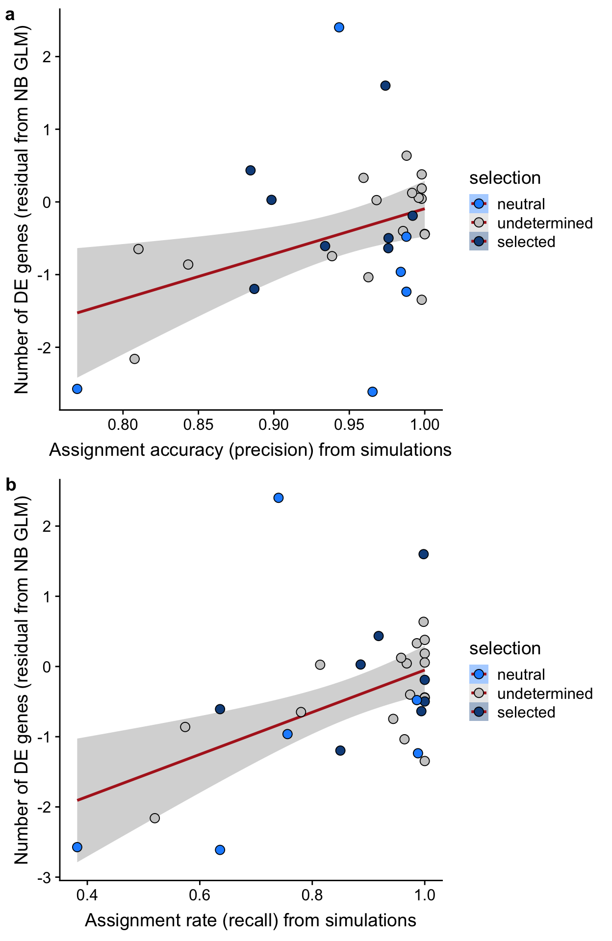

Expand here to see past versions of plot-de-assignment-acc-1.png:

Version	Author	Date
a056169	davismcc	2018-08-27

Linking DE to multiple explanatory factors

Let us fit a NB GLM to regress number of DE genes observed per line against number of cells, goodness of fit of selection models, number of somatic variants, assignment accuracy (from simulations) and assignment rate (observed) per line.

First we can look at fitting different combinations of these explanatory variables and do model selection using AIC (Akaike Information Criterion).

broom::glance(MASS::glm.nb(
  n_de_genes ~ n_cells + rsq_negbinfit + rsq_ntrtestr + nvars_all
  + recall_real + precision_simu, data = df))

# A tibble: 1 x 7
  null.deviance df.null logLik   AIC   BIC deviance df.residual
          <dbl>   <int>  <dbl> <dbl> <dbl>    <dbl>       <int>
1          53.0      30  -207.  431.  442.     37.4          24

broom::glance(MASS::glm.nb(
  n_de_genes ~ log10(n_cells) + rsq_negbinfit + rsq_ntrtestr + nvars_all
  + recall_real + precision_simu, data = df))

# A tibble: 1 x 7
  null.deviance df.null logLik   AIC   BIC deviance df.residual
          <dbl>   <int>  <dbl> <dbl> <dbl>    <dbl>       <int>
1          57.3      30  -206.  428.  439.     37.3          24

broom::glance(MASS::glm.nb(
  n_de_genes ~ sqrt(n_cells) + rsq_negbinfit + rsq_ntrtestr + nvars_all
  + recall_real + precision_simu, data = df))

# A tibble: 1 x 7
  null.deviance df.null logLik   AIC   BIC deviance df.residual
          <dbl>   <int>  <dbl> <dbl> <dbl>    <dbl>       <int>
1          54.8      30  -207.  430.  441.     37.4          24

broom::glance(MASS::glm.nb(
  n_de_genes ~ log10(n_cells) + rsq_negbinfit + rsq_ntrtestr + sqrt(nvars_all)
  + recall_real + precision_simu, data = df))

# A tibble: 1 x 7
  null.deviance df.null logLik   AIC   BIC deviance df.residual
          <dbl>   <int>  <dbl> <dbl> <dbl>    <dbl>       <int>
1          57.2      30  -206.  428.  439.     37.3          24

broom::glance(MASS::glm.nb(
  n_de_genes ~ log10(n_cells) + rsq_negbinfit + rsq_ntrtestr + log10(nvars_all)
  + recall_real + precision_simu, data = df))

# A tibble: 1 x 7
  null.deviance df.null logLik   AIC   BIC deviance df.residual
          <dbl>   <int>  <dbl> <dbl> <dbl>    <dbl>       <int>
1          57.1      30  -206.  428.  439.     37.3          24

broom::glance(MASS::glm.nb(
  n_de_genes ~ log10(n_cells) + rsq_ntrtestr + nvars_all
  + recall_real + precision_simu, data = df))

# A tibble: 1 x 7
  null.deviance df.null logLik   AIC   BIC deviance df.residual
          <dbl>   <int>  <dbl> <dbl> <dbl>    <dbl>       <int>
1          55.9      30  -206.  427.  437.     37.3          25

broom::glance(MASS::glm.nb(
  n_de_genes ~ log10(n_cells) + rsq_ntrtestr + nvars_all
  + recall_real, data = df))

# A tibble: 1 x 7
  null.deviance df.null logLik   AIC   BIC deviance df.residual
          <dbl>   <int>  <dbl> <dbl> <dbl>    <dbl>       <int>
1          54.1      30  -207.  426.  435.     37.4          26

broom::glance(MASS::glm.nb(
  n_de_genes ~ log10(n_cells) + rsq_ntrtestr + nvars_all, data = df))

# A tibble: 1 x 7
  null.deviance df.null logLik   AIC   BIC deviance df.residual
          <dbl>   <int>  <dbl> <dbl> <dbl>    <dbl>       <int>
1          53.8      30  -207.  424.  431.     37.4          27

broom::glance(MASS::glm.nb(
  n_de_genes ~ log10(n_cells) + rsq_negbinfit + nvars_all, data = df))

# A tibble: 1 x 7
  null.deviance df.null logLik   AIC   BIC deviance df.residual
          <dbl>   <int>  <dbl> <dbl> <dbl>    <dbl>       <int>
1          54.8      30  -207.  424.  431.     37.4          27

broom::glance(MASS::glm.nb(
  n_de_genes ~ log10(n_cells) + nvars_all, data = df))

# A tibble: 1 x 7
  null.deviance df.null logLik   AIC   BIC deviance df.residual
          <dbl>   <int>  <dbl> <dbl> <dbl>    <dbl>       <int>
1          53.6      30  -207.  422.  428.     37.4          28

broom::glance(MASS::glm.nb(
  n_de_genes ~ log10(n_cells), data = df))

# A tibble: 1 x 7
  null.deviance df.null logLik   AIC   BIC deviance df.residual
          <dbl>   <int>  <dbl> <dbl> <dbl>    <dbl>       <int>
1          51.3      30  -208.  422.  426.     37.5          29

The preferred model based on AIC values is one fitting log10-scale number of cells and number of somatic variants as predictor variables.

nbglm_nde_allfacts <- MASS::glm.nb(
  n_de_genes ~  log10(n_cells) + rsq_negbinfit + rsq_ntrtestr + nvars_all
  + recall_real + precision_simu, data = df)
broom::tidy(nbglm_nde_allfacts)

# A tibble: 7 x 5
  term           estimate std.error statistic  p.value
  <chr>             <dbl>     <dbl>     <dbl>    <dbl>
1 (Intercept)    -4.48      5.22       -0.857 0.391   
2 log10(n_cells)  4.53      1.34        3.38  0.000720
3 rsq_negbinfit   0.882     0.840       1.05  0.294   
4 rsq_ntrtestr   -2.29      2.60       -0.879 0.380   
5 nvars_all       0.00708   0.00723     0.980 0.327   
6 recall_real     0.283     2.06        0.138 0.891   
7 precision_simu  3.54      5.42        0.654 0.513

nbglm_nde_selectfacts <- MASS::glm.nb(
  n_de_genes ~ log10(n_cells) + nvars_all, data = df)
broom::tidy(nbglm_nde_selectfacts)

# A tibble: 3 x 5
  term           estimate std.error statistic   p.value
  <chr>             <dbl>     <dbl>     <dbl>     <dbl>
1 (Intercept)    -3.03      2.06        -1.47 0.141    
2 log10(n_cells)  4.91      1.25         3.93 0.0000835
3 nvars_all       0.00889   0.00724      1.23 0.219

broom::glance(nbglm_nde_selectfacts)

# A tibble: 1 x 7
  null.deviance df.null logLik   AIC   BIC deviance df.residual
          <dbl>   <int>  <dbl> <dbl> <dbl>    <dbl>       <int>
1          53.6      30  -207.  422.  428.     37.4          28

nbglm_nde_allfacts_tbl <- bind_cols(
  broom::tidy(nbglm_nde_selectfacts),
  broom::confint_tidy(nbglm_nde_selectfacts, conf.level = 0.9))


df_nbglm_nde <- broom::augment(nbglm_nde) %>%
  left_join(df_donor_info)

Linking pathway results to selection

Not yet implemented

Compare pathway results to clone prevalence

Hallmark gene sets. Not yet implemented.

Write DE and pathway results to file

## Write DE results to file:
for (don in names(de_res$qlf_list)) {
  de_res$qlf_list[[don]]$table %>% 
    dplyr::mutate(gene = rownames(.), FDR = IHW::adj_pvalues(IHW::ihw(PValue, logCPM, alpha = 0.1))) %>%
    dplyr::arrange(FDR) %>% write_tsv(
      paste0("output/differential_expression/", don, "_qlf_de_results.tsv"))
}

for (don in names(de_res$camera$H)) {
  for (cntrst in names(de_res$camera$H[[don]])) {
    de_res$camera$H[[don]][[cntrst]]$logFC %>% 
      dplyr::mutate(geneset = rownames(.)) %>%
      dplyr::arrange(FDR) %>% write_tsv(
        paste0("output/differential_expression/", don, "_camera_hallmark_geneset_results_", cntrst, ".tsv"))    
  }
}

Session information

devtools::session_info()

 setting  value                       
 version  R version 3.5.1 (2018-07-02)
 system   x86_64, darwin15.6.0        
 ui       X11                         
 language (EN)                        
 collate  en_GB.UTF-8                 
 tz       Europe/London               
 date     2018-11-09                  

 package              * version   date       source                
 AnnotationDbi        * 1.42.1    2018-05-08 Bioconductor          
 ape                    5.1       2018-04-04 CRAN (R 3.5.0)        
 assertthat             0.2.0     2017-04-11 CRAN (R 3.5.0)        
 backports              1.1.2     2017-12-13 CRAN (R 3.5.0)        
 base                 * 3.5.1     2018-07-05 local                 
 beeswarm               0.2.3     2016-04-25 CRAN (R 3.5.0)        
 bindr                  0.1.1     2018-03-13 CRAN (R 3.5.0)        
 bindrcpp             * 0.2.2     2018-03-29 CRAN (R 3.5.0)        
 Biobase              * 2.40.0    2018-05-01 Bioconductor          
 BiocGenerics         * 0.26.0    2018-05-01 Bioconductor          
 BiocParallel         * 1.14.2    2018-07-08 Bioconductor          
 biomaRt                2.36.1    2018-05-24 Bioconductor          
 Biostrings             2.48.0    2018-05-01 Bioconductor          
 bit                    1.1-14    2018-05-29 CRAN (R 3.5.0)        
 bit64                  0.9-7     2017-05-08 CRAN (R 3.5.0)        
 bitops                 1.0-6     2013-08-17 CRAN (R 3.5.0)        
 blob                   1.1.1     2018-03-25 CRAN (R 3.5.0)        
 broom                * 0.5.0     2018-07-17 CRAN (R 3.5.0)        
 BSgenome               1.48.0    2018-05-01 Bioconductor          
 cardelino            * 0.1.2     2018-08-21 Bioconductor          
 cellranger             1.1.0     2016-07-27 CRAN (R 3.5.0)        
 cli                    1.0.0     2017-11-05 CRAN (R 3.5.0)        
 colorspace             1.3-2     2016-12-14 CRAN (R 3.5.0)        
 compiler               3.5.1     2018-07-05 local                 
 cowplot              * 0.9.3     2018-07-15 CRAN (R 3.5.0)        
 crayon                 1.3.4     2017-09-16 CRAN (R 3.5.0)        
 crosstalk              1.0.0     2016-12-21 CRAN (R 3.5.0)        
 data.table             1.11.4    2018-05-27 CRAN (R 3.5.0)        
 datasets             * 3.5.1     2018-07-05 local                 
 DBI                    1.0.0     2018-05-02 CRAN (R 3.5.0)        
 DelayedArray         * 0.6.5     2018-08-15 Bioconductor          
 DelayedMatrixStats     1.2.0     2018-05-01 Bioconductor          
 devtools               1.13.6    2018-06-27 CRAN (R 3.5.0)        
 digest                 0.6.17    2018-09-12 CRAN (R 3.5.1)        
 dplyr                * 0.7.6     2018-06-29 CRAN (R 3.5.1)        
 DT                     0.4       2018-01-30 CRAN (R 3.5.0)        
 edgeR                * 3.22.3    2018-06-21 Bioconductor          
 evaluate               0.11      2018-07-17 CRAN (R 3.5.0)        
 fansi                  0.3.0     2018-08-13 CRAN (R 3.5.0)        
 fdrtool                1.2.15    2015-07-08 CRAN (R 3.5.0)        
 forcats              * 0.3.0     2018-02-19 CRAN (R 3.5.0)        
 gdtools              * 0.1.7     2018-02-27 CRAN (R 3.5.0)        
 GenomeInfoDb         * 1.16.0    2018-05-01 Bioconductor          
 GenomeInfoDbData       1.1.0     2018-04-25 Bioconductor          
 GenomicAlignments      1.16.0    2018-05-01 Bioconductor          
 GenomicFeatures        1.32.2    2018-08-13 Bioconductor          
 GenomicRanges        * 1.32.6    2018-07-20 Bioconductor          
 ggbeeswarm             0.6.0     2017-08-07 CRAN (R 3.5.0)        
 ggcorrplot           * 0.1.1     2016-01-12 CRAN (R 3.5.0)        
 ggforce              * 0.1.3     2018-07-07 CRAN (R 3.5.0)        
 ggplot2              * 3.0.0     2018-07-03 CRAN (R 3.5.0)        
 ggrepel              * 0.8.0     2018-05-09 CRAN (R 3.5.0)        
 ggridges             * 0.5.0     2018-04-05 CRAN (R 3.5.0)        
 ggthemes               4.0.1     2018-08-24 CRAN (R 3.5.1)        
 ggtree                 1.12.7    2018-08-07 Bioconductor          
 git2r                  0.23.0    2018-07-17 CRAN (R 3.5.0)        
 glue                   1.3.0     2018-07-17 CRAN (R 3.5.0)        
 graphics             * 3.5.1     2018-07-05 local                 
 grDevices            * 3.5.1     2018-07-05 local                 
 grid                   3.5.1     2018-07-05 local                 
 gridExtra              2.3       2017-09-09 CRAN (R 3.5.0)        
 gtable                 0.2.0     2016-02-26 CRAN (R 3.5.0)        
 haven                  1.1.2     2018-06-27 CRAN (R 3.5.0)        
 hms                    0.4.2     2018-03-10 CRAN (R 3.5.0)        
 htmltools              0.3.6     2017-04-28 CRAN (R 3.5.0)        
 htmlwidgets            1.2       2018-04-19 CRAN (R 3.5.0)        
 httpuv                 1.4.5     2018-07-19 CRAN (R 3.5.0)        
 httr                   1.3.1     2017-08-20 CRAN (R 3.5.0)        
 IHW                  * 1.8.0     2018-05-01 Bioconductor          
 IRanges              * 2.14.11   2018-08-24 Bioconductor          
 jsonlite               1.5       2017-06-01 CRAN (R 3.5.0)        
 knitr                  1.20      2018-02-20 CRAN (R 3.5.0)        
 labeling               0.3       2014-08-23 CRAN (R 3.5.0)        
 later                  0.7.3     2018-06-08 CRAN (R 3.5.0)        
 lattice                0.20-35   2017-03-25 CRAN (R 3.5.1)        
 lazyeval               0.2.1     2017-10-29 CRAN (R 3.5.0)        
 limma                * 3.36.3    2018-08-25 Bioconductor          
 locfit                 1.5-9.1   2013-04-20 CRAN (R 3.5.0)        
 lpsymphony             1.8.0     2018-05-01 Bioconductor (R 3.5.0)
 lubridate              1.7.4     2018-04-11 CRAN (R 3.5.0)        
 magrittr               1.5       2014-11-22 CRAN (R 3.5.0)        
 MASS                   7.3-50    2018-04-30 CRAN (R 3.5.1)        
 Matrix                 1.2-14    2018-04-13 CRAN (R 3.5.1)        
 matrixStats          * 0.54.0    2018-07-23 CRAN (R 3.5.0)        
 memoise                1.1.0     2017-04-21 CRAN (R 3.5.0)        
 methods              * 3.5.1     2018-07-05 local                 
 mime                   0.5       2016-07-07 CRAN (R 3.5.0)        
 modelr                 0.1.2     2018-05-11 CRAN (R 3.5.0)        
 munsell                0.5.0     2018-06-12 CRAN (R 3.5.0)        
 nlme                   3.1-137   2018-04-07 CRAN (R 3.5.1)        
 org.Hs.eg.db         * 3.6.0     2018-05-15 Bioconductor          
 parallel             * 3.5.1     2018-07-05 local                 
 pheatmap               1.0.10    2018-05-19 CRAN (R 3.5.0)        
 pillar                 1.3.0     2018-07-14 CRAN (R 3.5.0)        
 pkgconfig              2.0.2     2018-08-16 CRAN (R 3.5.0)        
 plyr                   1.8.4     2016-06-08 CRAN (R 3.5.0)        
 prettyunits            1.0.2     2015-07-13 CRAN (R 3.5.0)        
 progress               1.2.0     2018-06-14 CRAN (R 3.5.0)        
 promises               1.0.1     2018-04-13 CRAN (R 3.5.0)        
 purrr                * 0.2.5     2018-05-29 CRAN (R 3.5.0)        
 R.methodsS3            1.7.1     2016-02-16 CRAN (R 3.5.0)        
 R.oo                   1.22.0    2018-04-22 CRAN (R 3.5.0)        
 R.utils                2.7.0     2018-08-27 CRAN (R 3.5.0)        
 R6                     2.2.2     2017-06-17 CRAN (R 3.5.0)        
 RColorBrewer         * 1.1-2     2014-12-07 CRAN (R 3.5.0)        
 Rcpp                   0.12.18   2018-07-23 CRAN (R 3.5.0)        
 RCurl                  1.95-4.11 2018-07-15 CRAN (R 3.5.0)        
 readr                * 1.1.1     2017-05-16 CRAN (R 3.5.0)        
 readxl                 1.1.0     2018-04-20 CRAN (R 3.5.0)        
 reshape2               1.4.3     2017-12-11 CRAN (R 3.5.0)        
 rhdf5                  2.24.0    2018-05-01 Bioconductor          
 Rhdf5lib               1.2.1     2018-05-17 Bioconductor          
 rjson                  0.2.20    2018-06-08 CRAN (R 3.5.0)        
 rlang                * 0.2.2     2018-08-16 CRAN (R 3.5.0)        
 rmarkdown              1.10      2018-06-11 CRAN (R 3.5.0)        
 rprojroot              1.3-2     2018-01-03 CRAN (R 3.5.0)        
 Rsamtools              1.32.3    2018-08-22 Bioconductor          
 RSQLite                2.1.1     2018-05-06 CRAN (R 3.5.0)        
 rstudioapi             0.7       2017-09-07 CRAN (R 3.5.0)        
 rtracklayer            1.40.5    2018-08-20 Bioconductor          
 rvcheck                0.1.0     2018-05-23 CRAN (R 3.5.0)        
 rvest                  0.3.2     2016-06-17 CRAN (R 3.5.0)        
 S4Vectors            * 0.18.3    2018-06-08 Bioconductor          
 scales                 1.0.0     2018-08-09 CRAN (R 3.5.0)        
 scater               * 1.9.12    2018-08-03 Bioconductor          
 shiny                  1.1.0     2018-05-17 CRAN (R 3.5.0)        
 SingleCellExperiment * 1.2.0     2018-05-01 Bioconductor          
 slam                   0.1-43    2018-04-23 CRAN (R 3.5.0)        
 snpStats               1.30.0    2018-05-01 Bioconductor          
 splines                3.5.1     2018-07-05 local                 
 stats                * 3.5.1     2018-07-05 local                 
 stats4               * 3.5.1     2018-07-05 local                 
 stringi                1.2.4     2018-07-20 CRAN (R 3.5.0)        
 stringr              * 1.3.1     2018-05-10 CRAN (R 3.5.0)        
 SummarizedExperiment * 1.10.1    2018-05-11 Bioconductor          
 superheat            * 0.1.0     2017-02-04 CRAN (R 3.5.0)        
 survival               2.42-6    2018-07-13 CRAN (R 3.5.0)        
 svglite                1.2.1     2017-09-11 CRAN (R 3.5.0)        
 tibble               * 1.4.2     2018-01-22 CRAN (R 3.5.0)        
 tidyr                * 0.8.1     2018-05-18 CRAN (R 3.5.0)        
 tidyselect             0.2.4     2018-02-26 CRAN (R 3.5.0)        
 tidytree               0.1.9     2018-06-13 CRAN (R 3.5.0)        
 tidyverse            * 1.2.1     2017-11-14 CRAN (R 3.5.0)        
 tools                  3.5.1     2018-07-05 local                 
 treeio                 1.4.3     2018-08-13 Bioconductor          
 tweenr                 0.1.5     2016-10-10 CRAN (R 3.5.0)        
 tximport               1.8.0     2018-05-01 Bioconductor          
 units                  0.6-0     2018-06-09 CRAN (R 3.5.0)        
 utf8                   1.1.4     2018-05-24 CRAN (R 3.5.0)        
 utils                * 3.5.1     2018-07-05 local                 
 VariantAnnotation      1.26.1    2018-07-04 Bioconductor          
 vipor                  0.4.5     2017-03-22 CRAN (R 3.5.0)        
 viridis              * 0.5.1     2018-03-29 CRAN (R 3.5.0)        
 viridisLite          * 0.3.0     2018-02-01 CRAN (R 3.5.0)        
 whisker                0.3-2     2013-04-28 CRAN (R 3.5.0)        
 withr                  2.1.2     2018-03-15 CRAN (R 3.5.0)        
 workflowr              1.1.1     2018-07-06 CRAN (R 3.5.0)        
 XML                    3.98-1.16 2018-08-19 CRAN (R 3.5.1)        
 xml2                   1.2.0     2018-01-24 CRAN (R 3.5.0)        
 xtable                 1.8-3     2018-08-29 CRAN (R 3.5.1)        
 XVector                0.20.0    2018-05-01 Bioconductor          
 yaml                   2.2.0     2018-07-25 CRAN (R 3.5.1)        
 zlibbioc               1.26.0    2018-05-01 Bioconductor

This reproducible R Markdown analysis was created with workflowr 1.1.1