Simulation analysis: systematic and for all lines
Yuanhua Huang & Davis J. McCarthy
Last updated: 2018-08-27
workflowr checks: (Click a bullet for more information)-
✔ R Markdown file: up-to-date
Great! Since the R Markdown file has been committed to the Git repository, you know the exact version of the code that produced these results.
-
✔ Environment: empty
Great job! The global environment was empty. Objects defined in the global environment can affect the analysis in your R Markdown file in unknown ways. For reproduciblity it’s best to always run the code in an empty environment.
-
✔ Seed:
set.seed(20180807)The command
set.seed(20180807)was run prior to running the code in the R Markdown file. Setting a seed ensures that any results that rely on randomness, e.g. subsampling or permutations, are reproducible. -
✔ Session information: recorded
Great job! Recording the operating system, R version, and package versions is critical for reproducibility.
-
Great! You are using Git for version control. Tracking code development and connecting the code version to the results is critical for reproducibility. The version displayed above was the version of the Git repository at the time these results were generated.✔ Repository version: 678546d
Note that you need to be careful to ensure that all relevant files for the analysis have been committed to Git prior to generating the results (you can usewflow_publishorwflow_git_commit). workflowr only checks the R Markdown file, but you know if there are other scripts or data files that it depends on. Below is the status of the Git repository when the results were generated:
Note that any generated files, e.g. HTML, png, CSS, etc., are not included in this status report because it is ok for generated content to have uncommitted changes.Ignored files: Ignored: .DS_Store Ignored: .Rhistory Ignored: .Rproj.user/ Ignored: .vscode/ Ignored: code/.DS_Store Ignored: data/raw/ Ignored: src/.DS_Store Ignored: src/.ipynb_checkpoints/ Ignored: src/Rmd/.Rhistory Untracked files: Untracked: Snakefile_clonality Untracked: Snakefile_somatic_calling Untracked: code/analysis_for_garx.Rmd Untracked: code/selection/ Untracked: code/yuanhua/ Untracked: data/canopy/ Untracked: data/cell_assignment/ Untracked: data/de_analysis_FTv62/ Untracked: data/donor_info_070818.txt Untracked: data/donor_info_core.csv Untracked: data/donor_neutrality.tsv Untracked: data/exome-point-mutations/ Untracked: data/fdr10.annot.txt.gz Untracked: data/human_H_v5p2.rdata Untracked: data/human_c2_v5p2.rdata Untracked: data/human_c6_v5p2.rdata Untracked: data/neg-bin-rsquared-petr.csv Untracked: data/neutralitytestr-petr.tsv Untracked: data/sce_merged_donors_cardelino_donorid_all_qc_filt.rds Untracked: data/sce_merged_donors_cardelino_donorid_all_with_qc_labels.rds Untracked: data/sce_merged_donors_cardelino_donorid_unstim_qc_filt.rds Untracked: data/sces/ Untracked: data/selection/ Untracked: data/simulations/ Untracked: data/variance_components/ Untracked: figures/ Untracked: output/differential_expression/ Untracked: output/donor_specific/ Untracked: output/line_info.tsv Untracked: output/nvars_by_category_by_donor.tsv Untracked: output/nvars_by_category_by_line.tsv Untracked: output/variance_components/ Untracked: references/ Untracked: tree.txt
Expand here to see past versions:
| File | Version | Author | Date | Message |
|---|---|---|---|---|
| Rmd | 678546d | davismcc | 2018-08-27 | Suppressing warnings. |
| html | 9ec2a59 | davismcc | 2018-08-26 | Build site. |
| Rmd | cae617f | davismcc | 2018-08-26 | Updating simulation analyses |
| html | 36acf15 | davismcc | 2018-08-25 | Build site. |
| Rmd | d618fe5 | davismcc | 2018-08-25 | Updating analyses |
| html | 090c1b9 | davismcc | 2018-08-24 | Build site. |
| html | 02a8343 | davismcc | 2018-08-24 | Build site. |
| Rmd | 43f15d6 | davismcc | 2018-08-24 | Adding data pre-processing workflow and updating analyses. |
| html | 43f15d6 | davismcc | 2018-08-24 | Adding data pre-processing workflow and updating analyses. |
Load libraries and simulation results
knitr::opts_chunk$set(echo = TRUE, warning = FALSE, message = FALSE)
dir.create("figures/simulations", showWarnings = FALSE, recursive = TRUE)
library(ggpubr)
library(tidyverse)
library(cardelino)
library(viridis)
library(cowplot)
library(latex2exp)
lines <- c("euts", "fawm", "feec", "fikt", "garx", "gesg", "heja", "hipn",
            "ieki", "joxm", "kuco", "laey", "lexy", "naju", "nusw", "oaaz",
            "oilg", "pipw", "puie", "qayj", "qolg", "qonc", "rozh", "sehl",
            "ualf", "vass", "vuna", "wahn", "wetu", "xugn", "zoxy", "vils")
Simulation experiments
Define functions for simulation.
# assess cardelino with simulation
dat_dir <- "data/"
data(config_all)
data(simulation_input)
simu_input <- list("D" = D_input)

demuxlet <- function(A, D, Config, theta1 = 0.5, theta0 = 0.01) {
  P0_mat <- dbinom(A, D, theta0, log = TRUE)
  P1_mat <- dbinom(A, D, theta1, log = TRUE)
  P0_mat[which(is.na(P0_mat))] <- 0
  P1_mat[which(is.na(P1_mat))] <- 0
  logLik_mat <- t(P0_mat) %*% (1 - Config) + t(P1_mat) %*% Config
  prob_mat <- exp(logLik_mat) / rowSums(exp(logLik_mat))
  prob_mat
}

simulate_joint <- function(Config_all, D_all, n_clone = 4, mut_size = 5,
                           missing = NULL, error_mean = c(0.01, 0.44),
                           error_var = c(30, 4.8), n_repeat = 1) {
  simu_data_full <- list()
  for (i in seq_len(n_repeat)) {
    Config <- sample(Config_all[[n_clone - 2]], size = 1)[[1]]
    Config <- matrix(rep(c(t(Config)), mut_size), ncol = ncol(Config),
                     byrow = TRUE)
    row.names(Config) <- paste0("SNV", seq_len(nrow(Config)))
    colnames(Config) <- paste0("Clone", seq_len(ncol(Config)))
    D_input <- sample_seq_depth(D_all, n_cells = 200, missing_rate = missing,
                                n_sites = nrow(Config))
    sim_dat <- sim_read_count(Config, D_input, Psi = NULL, cell_num = 200,
                              means = error_mean, vars = error_var)
    sim_dat[["Config"]] <- Config
    simu_data_full[[i]] <- sim_dat
  }
  simu_data_full
}

assign_score <- function(prob_mat, simu_mat, threshold=0.2, mode="delta") {
  assign_0 <- cardelino::get_prob_label(simu_mat)
  assign_1 <- cardelino::get_prob_label(prob_mat)
  prob_val <- cardelino::get_prob_value(prob_mat, mode = mode)
  idx <- prob_val >= threshold

  rt_list <- list("ass" = mean(idx),
                  "acc" = mean(assign_0 == assign_1),
                  "acc_ass" = mean((assign_0 == assign_1)[idx]))
  rt_list
}

assign_curve <- function(prob_mat, simu_mat, mode="delta"){
  assign_0 <- cardelino::get_prob_label(simu_mat)
  assign_1 <- cardelino::get_prob_label(prob_mat)
  prob_val <- cardelino::get_prob_value(prob_mat, mode = mode)

  thresholds <- sort(unique(prob_val))
  ACC <- rep(0, length(thresholds))
  ASS <- rep(0, length(thresholds))
  for (i in seq_len(length(thresholds))) {
    idx <- prob_val >= thresholds[i]
    ASS[i] <- mean(idx)
    ACC[i] <- mean((assign_0 == assign_1)[idx])
  }
  thresholds <- c(thresholds, 1.0)
  ACC <- c(ACC, 1.0)
  ASS <- c(ASS, 0.0)
  AUC <- AUC_acc_ass <- 0.0
  for (i in seq_len(length(thresholds) - 1)) {
    AUC <- AUC + 0.5 * (thresholds[i] - thresholds[i + 1]) *
      (ACC[i] + ACC[i + 1])
    AUC_acc_ass <- AUC_acc_ass + 0.5 * (ASS[i] - ASS[i + 1]) *
      (ACC[i] + ACC[i + 1])
  }
  AUC <- AUC / (thresholds[1] - thresholds[length(thresholds)])
  AUC_acc_ass <- AUC_acc_ass / (ASS[1] - ASS[length(thresholds)])

  rt_list <- list("ACC" = ACC, "ASS" = ASS, "AUC" = AUC,
                  "AUC_acc_ass" = AUC_acc_ass, "thresholds" = thresholds)
  rt_list
}

assign_macro_ROC <- function(prob_mat, simu_mat) {
  thresholds <- seq(0, 0.999, 0.001)
  ACC <- rep(0, length(thresholds))
  ASS <- rep(0, length(thresholds))
  FPR <- rep(0, length(thresholds))
  TPR <- rep(0, length(thresholds))
  for (i in seq_len(length(thresholds))) {
    idx <- prob_mat >= thresholds[i]
    ASS[i] <- mean(idx) # not very meaningful
    ACC[i] <- mean(simu_mat[idx])
    FPR[i] <- sum(simu_mat[idx] == 0) / sum(simu_mat == 0)
    TPR[i] <- sum(simu_mat[idx] == 1) / sum(simu_mat == 1)
  }

  AUC <- 0.0
  for (i in seq_len(length(thresholds) - 1)) {
    AUC <- AUC + 0.5 * (FPR[i] - FPR[i + 1]) * (TPR[i] + TPR[i + 1])
  }

  rt_list <- list("FPR" = FPR, "TPR" = TPR, "AUC" = AUC,
                  "thresholds" = thresholds, "ACC" = ACC, "ASS" = ASS)
  rt_list
}
Run simulations.
set.seed(1)
ACC_all <- c()
ASS_all <- c()
AUC_all <- c()
ERR_all <- c()
labels_all <- c()
method_all <- c()
variable_all <- c()

type_use <- c("mut_size", "n_clone", "missing", "FNR", "shapes1")
value_list <- list(c(3, 5, 7, 10, 15, 25),
                   seq(3, 8),
                   seq(0.7, 0.95, 0.05),
                   seq(0.35, 0.6, 0.05),
                   c(0.5, 1.0, 2.0, 4.0, 8.0, 16.0))

for (mm in seq_len(length(value_list))) {
  values_all <- value_list[[mm]]
  for (k in seq_len(length(values_all)))  {
    if (mm == 1) {
      simu_data <- simulate_joint(Config_all, simu_input$D, n_clone = 4,
                                  mut_size = values_all[k], missing = 0.8,
                                  error_mean = c(0.01, 0.44), n_repeat = 20)
    } else if (mm == 2) {
      simu_data <- simulate_joint(Config_all, simu_input$D,
                                  n_clone = values_all[k], mut_size = 10,
                                  missing = 0.8, error_mean = c(0.01, 0.44),
                                  n_repeat = 20)
    } else if (mm == 3) {
      simu_data <- simulate_joint(Config_all, simu_input$D, n_clone = 4,
                                  mut_size = 10, missing = values_all[k],
                                  error_mean = c(0.01, 0.44), n_repeat = 20)
    } else if (mm == 4) {
      simu_data <- simulate_joint(Config_all, simu_input$D, n_clone = 4,
                                  mut_size = 10, missing = 0.8,
                                  error_mean = c(0.01, values_all[k]),
                                  n_repeat = 20)
    } else if (mm == 5) {
      simu_data <- simulate_joint(Config_all, simu_input$D, n_clone = 4,
                                  mut_size = 10, missing = 0.8,
                                  error_mean = c(0.01, 0.44),
                                  error_var = c(30, values_all[k]),
                                  n_repeat = 20)
    }

    for (d_tmp in simu_data) {
      prob_all <- list()
      methods_use <- c("demuxlet", "Bern_EM", "Binom_EM", "Binom_Gibbs",
                       "Binom_gmline")
      prob_all[[1]] <- demuxlet(d_tmp$A_sim, d_tmp$D_sim, d_tmp$Config,
                                theta0 = mean(d_tmp$theta0_binom, na.rm = TRUE))
      prob_all[[2]] <- cell_assign_EM(d_tmp$A_sim, d_tmp$D_sim, d_tmp$Config,
                                      Psi = NULL, verbose = F)$prob
      prob_all[[3]] <- cell_assign_EM(d_tmp$A_sim, d_tmp$D_sim, d_tmp$Config,
                                      Psi = NULL, model = "binomial",
                                      verbose = FALSE)$prob
      prob_all[[4]] <- cell_assign_Gibbs(d_tmp$A_sim, d_tmp$D_sim,
                                         d_tmp$Config, Psi = NULL,
                                         min_iter = 1000, wise = "variant",
                                         prior1 = c(2.11, 2.69),
                                         verbose = FALSE)$prob

      for (i in seq_len(length(prob_all))) {
        prob_mat <- prob_all[[i]]
        assign_scr <- assign_score(prob_mat, d_tmp$I_sim,
                                                threshold = 0.5001,
                                                mode = "best")
        ACC_all <- c(ACC_all, assign_scr$acc_ass)
        ASS_all <- c(ASS_all, assign_scr$ass)
        AUC_all <- c(AUC_all, assign_curve(prob_mat, d_tmp$I_sim,
                                           mode = "best")$AUC_acc_ass)
        ERR_all <- c(ERR_all, mean(abs(prob_mat - d_tmp$I_sim)))
        labels_all <- c(labels_all, values_all[k])
        method_all <- c(method_all, methods_use[i])
        variable_all <- c(variable_all, type_use[mm])
      }
    }
  }
}

df <- data.frame(Accuracy = ACC_all, AUC_of_ACC_ASS = AUC_all,
                 Assignable = ASS_all, MAE = ERR_all, Methods = method_all,
                 labels = labels_all, variable = variable_all)

dat_dir <- "data/simulations"
saveRDS(df, paste0(dat_dir, "/simulate_extra_s1_v2.rds"))
Precision-recall curve
set.seed(1)
PCAU_curve_list <- list()

simu_data <- simulate_joint(Config_all, simu_input$D, n_clone = 4,
                              mut_size = 10, missing = 0.8,
                              error_mean = c(0.01, 0.44), n_repeat = 20)

assign_0 <- matrix(0, nrow = 200, ncol = 20)
assign_1 <- matrix(0, nrow = 200, ncol = 20)
prob_all <- matrix(0, nrow = 200, ncol = 20)
for (i in seq_len(length(simu_data))) {
  d_tmp <- simu_data[[i]]
  prob_tmp <- cell_assign_Gibbs(d_tmp$A_sim, d_tmp$D_sim,
                                d_tmp$Config, Psi = NULL,
                                min_iter = 1000, wise = "variant",
                                prior1 = c(2.11, 2.69), verbose = FALSE)$prob
  assign_0[, i] <- get_prob_label(d_tmp$I_sim)
  assign_1[, i] <- get_prob_label(prob_tmp)
  prob_all[, i] <- get_prob_value(prob_tmp, mode = "best")
}

dat_dir = "data/simulations"
saveRDS(list("assign_0" = assign_0, "assign_1" = assign_1,
             "prob_all" = prob_all),
        paste0(dat_dir, "/simulate_prob_curve.rds"))
Analysis of systematic results
Precision-recall curve for default settings
rds.tmp <- readRDS(paste0(dat_dir, "/simulate_prob_curve.rds"))
assign_0 <- rds.tmp$assign_0
assign_1 <- rds.tmp$assign_1
prob_all <- rds.tmp$prob_all

thresholds <- seq(0, 1, 0.001)
recalls <- rep(0, length(thresholds))
precision_all <- matrix(0, nrow = length(thresholds), ncol = ncol(prob_all) + 1)
for (i in seq_len(length(thresholds))) {
    idx <- prob_all >= thresholds[i]
    recalls[i] <- mean(idx)
    precision_all[i, ncol(prob_all) + 1] <- mean((assign_0 == assign_1)[idx])
    for (j in seq_len(ncol(prob_all))) {
        idx <- prob_all[, j] >= sort(prob_all[, j],
                                     decreasing = TRUE)[round(recalls[i] *
                                                                nrow(prob_all))]
        precision_all[i, j] <- mean((assign_0[,j] == assign_1[,j])[idx])
    }
}

order_idx <- order(colMeans(precision_all[, 1:ncol(prob_all)]))
idx1 <- order_idx[round(0.25 * length(order_idx))]
idx2 <- order_idx[round(0.75 * length(order_idx))]

df.tmp <- data.frame(cutoff = thresholds, Recall = recalls,
                     Presision = precision_all[, ncol(precision_all)],
                     ACC_low1 = precision_all[, idx1],
                     ACC_high1 = precision_all[, idx2])
Calculate AUC score.
nn <- ncol(precision_all)
AUC_score <- 0.0
for (i in seq_len(length(recalls) - 1)) {
    AUC_score <- AUC_score + 0.5 * (recalls[i] - recalls[i + 1]) *
      (precision_all[i, nn] + precision_all[i + 1, nn])
}
AUC_score <- AUC_score / (recalls[1] - recalls[length(recalls)])
print(AUC_score)
[1] 0.9469786Plot PR curve.
fig_dir <- "figures/simulations"

idx_05 <- prob_all >= 0.5
recall_05 <- mean(idx_05)
precision_05 <- mean((assign_0 == assign_1)[idx_05])
print(c(recall_05, precision_05))
[1] 0.7902500 0.8895919fig.curve <- ggplot(df.tmp, aes(x = Recall, y = Presision)) +
geom_ribbon(aes(ymin = ACC_low1, ymax = ACC_high1), fill = "grey80") +
scale_color_viridis(option = "B") +
geom_line(aes(color = cutoff)) + geom_point(aes(color = cutoff), size = 0.5) +
geom_point(aes(x = recall_05, y = precision_05), shape = 1, color = "black",
size = 3) +
xlab("Recall: Fraction of assignable cells") +
ylab("Precision") +
ylim(0.5, 1) +
pub.theme() +
theme(legend.position = c(0.25,0.45)) +
labs(color = 'highest P')
ggsave(paste0(fig_dir, "/fig1b_PRcurve.png"),
fig.curve, height = 2.5, width = 3.5, dpi = 300)
ggsave(paste0(fig_dir, "/fig1b_PRcurve.pdf"),
fig.curve, height = 2.5, width = 3.5, dpi = 300)
fig.curve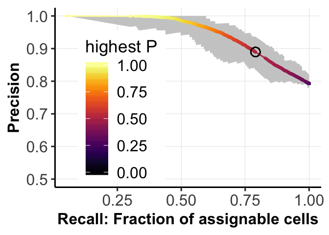
Expand here to see past versions of plot-pr-curve-1.png:
| Version | Author | Date |
|---|---|---|
| 9ec2a59 | davismcc | 2018-08-26 |
Comparison of parameters
Assess cardelino with simulated data.
df <- readRDS(paste0("data/simulations/simulate_extra_s1_v2.rds"))

## Change method names
df$Methods <- as.character(df$Methods)
df <- df[df$Methods != "Bern_EM", ]
df$Methods[df$Methods == "demuxlet"] <- "theta_fixed"
df$Methods[df$Methods == "Binom_EM"] <- "theta_EM"
df$Methods[df$Methods == "Binom_Gibbs"] <- "cardelino"
df$Methods <- as.factor(df$Methods)

## Change variables
df$labels[df$variable == "missing"] <- 1 - df$labels[df$variable == "missing"]
df$labels[df$variable == "shapes1"] <- 1 / df$labels[df$variable == "shapes1"] #paste0("1/", df$labels[df$variable == "shapes1"])
Table of results from simulations:
head(df) Accuracy AUC_of_ACC_ASS Assignable MAE Methods labels
1 0.8600000 0.6958512 0.250 0.2976787 theta_fixed 3
3 0.8600000 0.6906667 0.250 0.2990589 theta_EM 3
4 0.8571429 0.6900893 0.245 0.2992734 cardelino 3
5 0.9142857 0.8002719 0.350 0.2139113 theta_fixed 3
7 0.9295775 0.8078752 0.355 0.2109320 theta_EM 3
8 0.9295775 0.8107345 0.355 0.2087012 cardelino 3
variable
1 mut_size
3 mut_size
4 mut_size
5 mut_size
7 mut_size
8 mut_sizeArea under Precision-Recall curves for different parameter settings.
fig_dir <- "figures/simulations/"

df1 <- df[df$Methods == "cardelino", ]

type_use <- c("mut_size", "n_clone", "missing", "FNR", "shapes1")
xlabels <- c("# variants per clonal branch", "Number of clones",
             "Overall variant coverage")
titles <- c("Mutations per branch", "Numbers of clones", "Variant coverages",
            "Fraction of ALT allele", "Constrentration of allelic expr")

df1 <- df1[df1$labels != 40, ]
df1 <- df1[df1$labels != 0.65, ]
df1 <- df1[df1$labels != 0.60, ]

fig_list <- list()
for (mm in c(1,3)) {
  fig_list[[mm]] <- ggplot(df1[df1$variable == type_use[mm], ],
                           aes(x = as.factor(labels), y = AUC_of_ACC_ASS)) +
    ylab("AU precision-recall curve") +
    geom_boxplot() + xlab(xlabels[mm]) +
    ylim(0.6, 1) + pub.theme()
  #     if (mm == 1) {
  #         fig_list[[mm]] <- fig_list[[mm]] +
  #             scale_x_discrete(labels=c("3", "5", "7", "10*", "15", "15")) }
  #     if (mm == 3) {
  #         fig_list[[mm]] <- fig_list[[mm]] +
  #             scale_x_discrete(labels=c("0.05", "0.1", "0.15", "0.2*", "0.25", "0.3")) }
}

ggsave(file = paste0(fig_dir, "fig_1c_mutations.png"),
       fig_list[[1]], height = 2.5, width = 3.5, dpi = 300)
ggsave(file = paste0(fig_dir, "fig_1c_mutations.pdf"),
       fig_list[[1]], height = 2.5, width = 3.5, dpi = 300)

ggsave(file = paste0(fig_dir, "fig_1d_coverages.png"),
       fig_list[[3]], height = 2.5, width = 3.5, dpi = 300)
ggsave(file = paste0(fig_dir, "fig_1d_coverages.pdf"),
       fig_list[[3]], height = 2.5, width = 3.5, dpi = 300)

fig_list[[1]]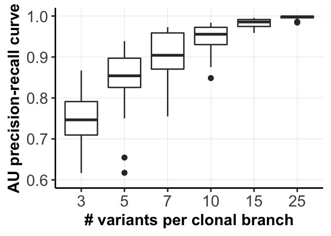
Expand here to see past versions of fig1d-1.png:
| Version | Author | Date |
|---|---|---|
| 9ec2a59 | davismcc | 2018-08-26 |
fig_list[[3]]
Expand here to see past versions of fig1d-2.png:
| Version | Author | Date |
|---|---|---|
| 9ec2a59 | davismcc | 2018-08-26 |
Boxplots comparing different models for cell-clone assignment.
type_use <- c("mut_size", "n_clone", "missing", "FNR", "shapes1")
xlabels <- c("# variants per clonal branch", "Number of clones",
             "Overall variant coverage",
             "Mean fraction of ALT alleles", "Variance of allelic imbalance")
df$Methods <- ordered(df$Methods, levels=c("theta_fixed", "theta_EM",
                                           "cardelino")) #Bern_EM

xlabel_list <- list(c("3", "5", "7", "10*", "15", "15"),
                    c("3", "4*", "5", "6", "7", "8"),
                    c("0.05", "0.1", "0.15", "0.2*", "0.25", "0.3"),
                    c("0.35", "0.4", "* 0.45", "0.5", "0.55", "0.6"),
                    c("1/16", "1/8", "*  1/4", "1/2", "1", "2"))

fig_list <- list()
for (mm in seq_len(length(type_use))) {
  fig_list[[mm]] <- ggplot(df[df$variable == type_use[mm], ],
                           aes(x = as.factor(labels), y = AUC_of_ACC_ASS,
                               fill=Methods)) +
    geom_boxplot() + xlab(xlabels[mm]) + ylab("AUC: precision-recall curve") +
    pub.theme() +
    scale_fill_brewer() +
    scale_x_discrete(labels=xlabel_list[[mm]])
}

fig_box <- ggarrange(fig_list[[1]], fig_list[[3]], fig_list[[2]],
                     fig_list[[4]], fig_list[[5]],
                     labels = c("A", "B", "C", "D", "E"),
                     nrow = 2, ncol = 3, align = "hv",
                     common.legend = TRUE, legend = "bottom")

ggsave(file = paste0(fig_dir, "simulation_overall_AUC.png"),
       fig_box, height = 7, width = 12, dpi = 300)
ggsave(file = paste0(fig_dir, "simulation_overall_AUC.pdf"),
       fig_box, height = 7, width = 12, dpi = 300)

fig_box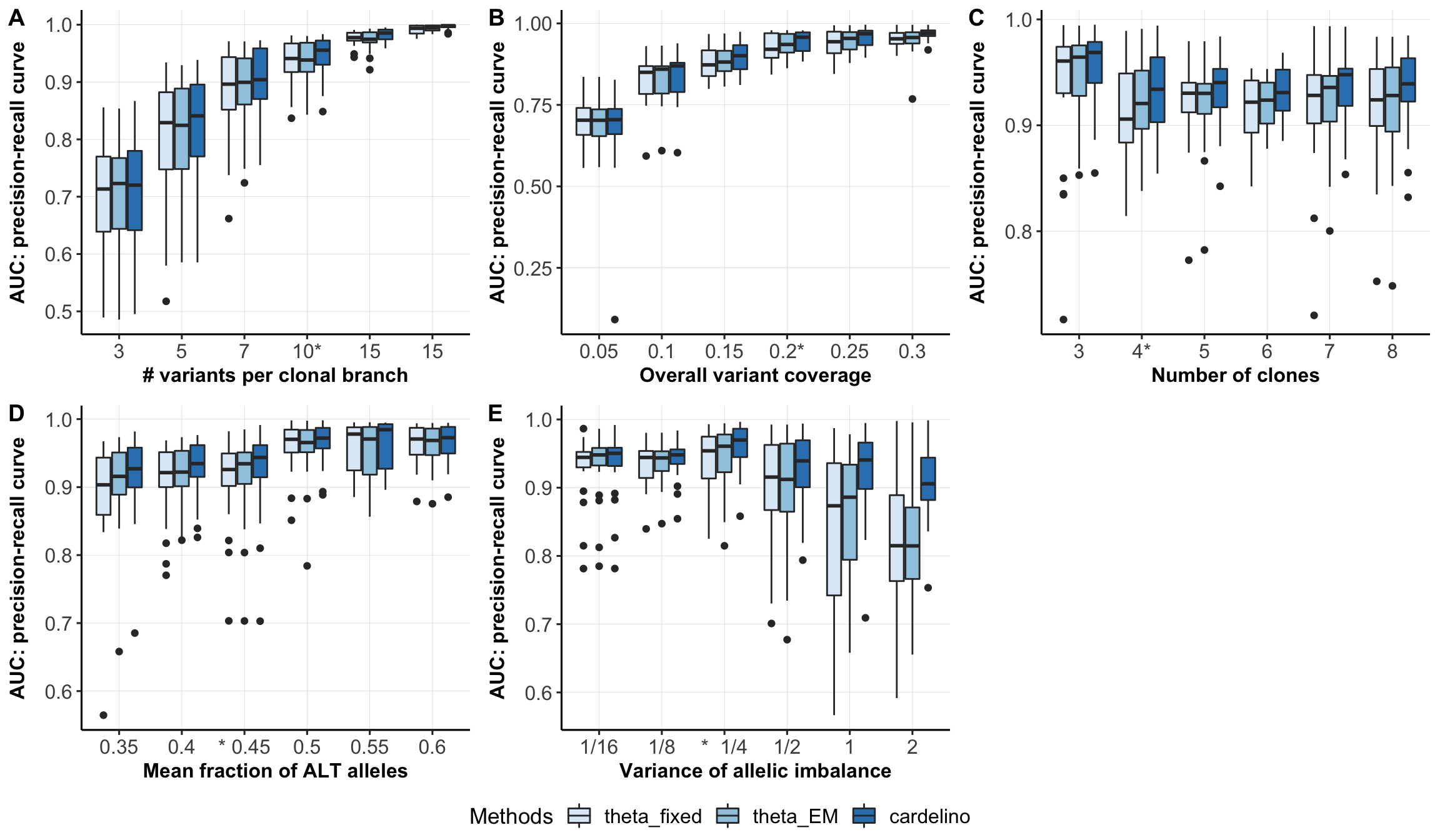
Expand here to see past versions of unnamed-chunk-6-1.png:
| Version | Author | Date |
|---|---|---|
| 9ec2a59 | davismcc | 2018-08-26 |
Analysis of simulation results for individual lines
Load simulation results for individual lines
all_files <- paste0(lines, ".simulate.rds")
assign_0 <- matrix(0, nrow = 500, ncol = length(lines))
assign_1 <- matrix(0, nrow = 500, ncol = length(lines))
prob_all <- matrix(0, nrow = 500, ncol = length(lines))

for (i in seq_len(length(all_files))) {
  afile <- all_files[i]
  sim_dat <- readRDS(file.path("data", "simulations", afile))
  assign_0[, i] <- get_prob_label(sim_dat$I_sim)
  assign_1[, i] <- get_prob_label(sim_dat$prob_Gibbs)
  prob_all[, i] <- get_prob_value(sim_dat$prob_Gibbs, mode = "best")
}
Load results from real data
all_files <- paste0("cardelino_results.", lines,
                    ".filt_lenient.cell_coverage_sites.rds")
n_sites <- rep(0, length(lines))
n_clone <- rep(0, length(lines))
recall_all <- rep(0, length(lines))
for (i in seq_len(length(all_files))) {
  afile <- all_files[i]
  carde_dat <- readRDS(file.path("data", "cell_assignment", afile))
  n_sites[i] <- nrow(carde_dat$D)
  n_clone[i] <- ncol(carde_dat$prob_mat)
  recall_all[i] <- mean(get_prob_value(carde_dat$prob_mat, mode = "best") > 0.5)
}
Overall correlation in assignment rates (recall) from simulated and observed data is 0.959.
precision_simu <- rep(0, length(lines))
for (i in seq_len(length(lines))) {
  idx <- prob_all[, i] > 0.5
  precision_simu[i] <- mean(assign_0[idx, i] == assign_1[idx, i])
}

df <- data.frame(line = lines, n_sites = n_sites, n_clone = n_clone,
                 recall_real = recall_all, recall_simu = colMeans(prob_all > 0.5),
                 precision_simu = precision_simu)
Plot observed vs simulated assignment rates (recall)
df %>%
  dplyr::mutate(sites_per_clone = cut(n_sites / pmax(n_clone - 1, 1),
                                      breaks = c(0, 3, 8, 15, 25, 60))) %>%
  ggplot(
         aes(x = recall_simu, y = recall_real,
             fill = sites_per_clone)) +
  geom_abline(slope = 1, intercept = 0, colour = "gray40", linetype = 2) +
  geom_smooth(aes(group = 1), method = "lm", colour = "firebrick") +
  geom_point(size = 3, shape = 21) +
  xlim(0, 1) + ylim(0, 1) +
  scale_fill_manual(name = "mean\n# variants\nper clonal\nbranch",
                    values = magma(6)[-1]) +
  guides(colour = FALSE, group = FALSE) +
  xlab("Assignment rate: simulated") +
  ylab("Assignment rate: observed")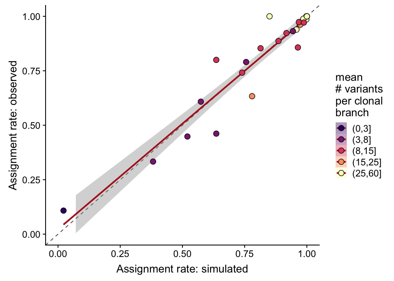
Expand here to see past versions of unnamed-chunk-10-1.png:
| Version | Author | Date |
|---|---|---|
| 9ec2a59 | davismcc | 2018-08-26 |
ggsave("figures/simulations/assign_rate_obs_v_sim.png",
       height = 4.5, width = 5)
ggsave("figures/simulations/assign_rate_obs_v_sim.pdf",
       height = 4.5, width = 5)
Plot simulation precision-recall curve
df %>%
  dplyr::mutate(sites_per_clone = cut(n_sites / n_clone,
                                      breaks = c(0, 5, 10, 20, 40))) %>%
  ggplot(
         aes(x = recall_simu, y = precision_simu,
             fill = sites_per_clone)) +
  geom_hline(yintercept = 0.85, colour = "gray40", linetype = 2) +
  geom_smooth(aes(group = 1), method = "lm", colour = "firebrick") +
  geom_point(size = 3, shape = 21) +
  xlim(0, 1) + ylim(0, 1) +
  scale_fill_manual(name = "mean\n# variants\nper clone",
                    values = magma(5)[-1]) +
  guides(colour = FALSE, group = FALSE) +
  xlab("Assignment rate (recall)") +
  ylab("Precision")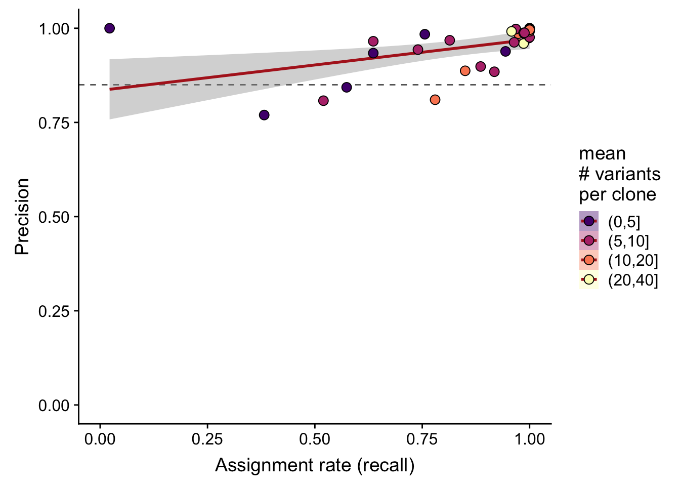
Expand here to see past versions of unnamed-chunk-11-1.png:
| Version | Author | Date |
|---|---|---|
| 9ec2a59 | davismcc | 2018-08-26 |
ggsave("figures/simulations/sim_precision_v_recall.png",
       height = 4.5, width = 5.5)
ggsave("figures/simulations/sim_precision_v_recall.pdf",
       height = 4.5, width = 5.5)
Clone statistics
Table showing the number of lines with 2, 3 and 4 clones.
table(df$n_clone)
 2  3  4
 4 24  4
Summary of the average number of mutations per clonal branch across lines.
summary(df$n_sites / (df$n_clone - 1)) Min. 1st Qu. Median Mean 3rd Qu. Max.
3.00 8.50 11.50 18.69 25.00 57.50 Session information
devtools::session_info() setting value
version R version 3.5.1 (2018-07-02)
system x86_64, darwin15.6.0
ui X11
language (EN)
collate en_GB.UTF-8
tz Europe/London
date 2018-08-27
package * version date source
AnnotationDbi 1.42.1 2018-05-08 Bioconductor
ape 5.1 2018-04-04 CRAN (R 3.5.0)
assertthat 0.2.0 2017-04-11 CRAN (R 3.5.0)
backports 1.1.2 2017-12-13 CRAN (R 3.5.0)
base * 3.5.1 2018-07-05 local
bindr 0.1.1 2018-03-13 CRAN (R 3.5.0)
bindrcpp * 0.2.2 2018-03-29 CRAN (R 3.5.0)
Biobase 2.40.0 2018-05-01 Bioconductor
BiocGenerics 0.26.0 2018-05-01 Bioconductor
BiocParallel 1.14.2 2018-07-08 Bioconductor
biomaRt 2.36.1 2018-05-24 Bioconductor
Biostrings 2.48.0 2018-05-01 Bioconductor
bit 1.1-14 2018-05-29 CRAN (R 3.5.0)
bit64 0.9-7 2017-05-08 CRAN (R 3.5.0)
bitops 1.0-6 2013-08-17 CRAN (R 3.5.0)
blob 1.1.1 2018-03-25 CRAN (R 3.5.0)
broom 0.5.0 2018-07-17 CRAN (R 3.5.0)
BSgenome 1.48.0 2018-05-01 Bioconductor
cardelino * 0.1.2 2018-08-21 Bioconductor
cellranger 1.1.0 2016-07-27 CRAN (R 3.5.0)
cli 1.0.0 2017-11-05 CRAN (R 3.5.0)
colorspace 1.3-2 2016-12-14 CRAN (R 3.5.0)
compiler 3.5.1 2018-07-05 local
cowplot * 0.9.3 2018-07-15 CRAN (R 3.5.0)
crayon 1.3.4 2017-09-16 CRAN (R 3.5.0)
datasets * 3.5.1 2018-07-05 local
DBI 1.0.0 2018-05-02 CRAN (R 3.5.0)
DelayedArray 0.6.5 2018-08-15 Bioconductor
devtools 1.13.6 2018-06-27 CRAN (R 3.5.0)
digest 0.6.16 2018-08-22 CRAN (R 3.5.0)
dplyr * 0.7.6 2018-06-29 CRAN (R 3.5.1)
evaluate 0.11 2018-07-17 CRAN (R 3.5.0)
forcats * 0.3.0 2018-02-19 CRAN (R 3.5.0)
GenomeInfoDb 1.16.0 2018-05-01 Bioconductor
GenomeInfoDbData 1.1.0 2018-04-25 Bioconductor
GenomicAlignments 1.16.0 2018-05-01 Bioconductor
GenomicFeatures 1.32.2 2018-08-13 Bioconductor
GenomicRanges 1.32.6 2018-07-20 Bioconductor
ggplot2 * 3.0.0 2018-07-03 CRAN (R 3.5.0)
ggpubr * 0.1.7 2018-06-23 CRAN (R 3.5.0)
ggtree 1.12.7 2018-08-07 Bioconductor
git2r 0.23.0 2018-07-17 CRAN (R 3.5.0)
glue 1.3.0 2018-07-17 CRAN (R 3.5.0)
graphics * 3.5.1 2018-07-05 local
grDevices * 3.5.1 2018-07-05 local
grid 3.5.1 2018-07-05 local
gridExtra 2.3 2017-09-09 CRAN (R 3.5.0)
gtable 0.2.0 2016-02-26 CRAN (R 3.5.0)
haven 1.1.2 2018-06-27 CRAN (R 3.5.0)
hms 0.4.2 2018-03-10 CRAN (R 3.5.0)
htmltools 0.3.6 2017-04-28 CRAN (R 3.5.0)
httr 1.3.1 2017-08-20 CRAN (R 3.5.0)
IRanges 2.14.11 2018-08-24 Bioconductor
jsonlite 1.5 2017-06-01 CRAN (R 3.5.0)
knitr 1.20 2018-02-20 CRAN (R 3.5.0)
labeling 0.3 2014-08-23 CRAN (R 3.5.0)
latex2exp * 0.4.0 2015-11-30 CRAN (R 3.5.0)
lattice 0.20-35 2017-03-25 CRAN (R 3.5.1)
lazyeval 0.2.1 2017-10-29 CRAN (R 3.5.0)
lubridate 1.7.4 2018-04-11 CRAN (R 3.5.0)
magrittr * 1.5 2014-11-22 CRAN (R 3.5.0)
Matrix 1.2-14 2018-04-13 CRAN (R 3.5.1)
matrixStats 0.54.0 2018-07-23 CRAN (R 3.5.0)
memoise 1.1.0 2017-04-21 CRAN (R 3.5.0)
methods * 3.5.1 2018-07-05 local
modelr 0.1.2 2018-05-11 CRAN (R 3.5.0)
munsell 0.5.0 2018-06-12 CRAN (R 3.5.0)
nlme 3.1-137 2018-04-07 CRAN (R 3.5.1)
parallel 3.5.1 2018-07-05 local
pheatmap 1.0.10 2018-05-19 CRAN (R 3.5.0)
pillar 1.3.0 2018-07-14 CRAN (R 3.5.0)
pkgconfig 2.0.2 2018-08-16 CRAN (R 3.5.0)
plyr 1.8.4 2016-06-08 CRAN (R 3.5.0)
prettyunits 1.0.2 2015-07-13 CRAN (R 3.5.0)
progress 1.2.0 2018-06-14 CRAN (R 3.5.0)
purrr * 0.2.5 2018-05-29 CRAN (R 3.5.0)
R.methodsS3 1.7.1 2016-02-16 CRAN (R 3.5.0)
R.oo 1.22.0 2018-04-22 CRAN (R 3.5.0)
R.utils 2.6.0 2017-11-05 CRAN (R 3.5.0)
R6 2.2.2 2017-06-17 CRAN (R 3.5.0)
RColorBrewer 1.1-2 2014-12-07 CRAN (R 3.5.0)
Rcpp 0.12.18 2018-07-23 CRAN (R 3.5.0)
RCurl 1.95-4.11 2018-07-15 CRAN (R 3.5.0)
readr * 1.1.1 2017-05-16 CRAN (R 3.5.0)
readxl 1.1.0 2018-04-20 CRAN (R 3.5.0)
rlang 0.2.2 2018-08-16 CRAN (R 3.5.0)
rmarkdown 1.10 2018-06-11 CRAN (R 3.5.0)
rprojroot 1.3-2 2018-01-03 CRAN (R 3.5.0)
Rsamtools 1.32.3 2018-08-22 Bioconductor
RSQLite 2.1.1 2018-05-06 CRAN (R 3.5.0)
rstudioapi 0.7 2017-09-07 CRAN (R 3.5.0)
rtracklayer 1.40.5 2018-08-20 Bioconductor
rvcheck 0.1.0 2018-05-23 CRAN (R 3.5.0)
rvest 0.3.2 2016-06-17 CRAN (R 3.5.0)
S4Vectors 0.18.3 2018-06-08 Bioconductor
scales 1.0.0 2018-08-09 CRAN (R 3.5.0)
snpStats 1.30.0 2018-05-01 Bioconductor
splines 3.5.1 2018-07-05 local
stats * 3.5.1 2018-07-05 local
stats4 3.5.1 2018-07-05 local
stringi 1.2.4 2018-07-20 CRAN (R 3.5.0)
stringr * 1.3.1 2018-05-10 CRAN (R 3.5.0)
SummarizedExperiment 1.10.1 2018-05-11 Bioconductor
survival 2.42-6 2018-07-13 CRAN (R 3.5.0)
tibble * 1.4.2 2018-01-22 CRAN (R 3.5.0)
tidyr * 0.8.1 2018-05-18 CRAN (R 3.5.0)
tidyselect 0.2.4 2018-02-26 CRAN (R 3.5.0)
tidytree 0.1.9 2018-06-13 CRAN (R 3.5.0)
tidyverse * 1.2.1 2017-11-14 CRAN (R 3.5.0)
tools 3.5.1 2018-07-05 local
treeio 1.4.3 2018-08-13 Bioconductor
utils * 3.5.1 2018-07-05 local
VariantAnnotation 1.26.1 2018-07-04 Bioconductor
viridis * 0.5.1 2018-03-29 CRAN (R 3.5.0)
viridisLite * 0.3.0 2018-02-01 CRAN (R 3.5.0)
whisker 0.3-2 2013-04-28 CRAN (R 3.5.0)
withr 2.1.2 2018-03-15 CRAN (R 3.5.0)
workflowr 1.1.1 2018-07-06 CRAN (R 3.5.0)
XML 3.98-1.16 2018-08-19 CRAN (R 3.5.1)
xml2 1.2.0 2018-01-24 CRAN (R 3.5.0)
XVector 0.20.0 2018-05-01 Bioconductor
yaml 2.2.0 2018-07-25 CRAN (R 3.5.1)
zlibbioc 1.26.0 2018-05-01 Bioconductor This reproducible R Markdown analysis was created with workflowr 1.1.1